Article

Optimising the Workflow for Fish Detection in DIDSON (Dual-Frequency IDentification SONar) Data with the Use of Optical Flow and a Genetic Algorithm

by
Triantafyllia-Maria Perivolioti
1,*,
Michal Tušer
2,
Dimitrios Terzopoulos
3,
Stefanos P. Sgardelis
4 and
Ioannis Antoniou
5
1
Department of Zoology, School of Biology, Aristotle University of Thessaloniki, 54124 Thessaloniki, Greece
2
Biology Centre of the Czech Academy of Sciences, Institute of Hydrobiology, 37005 České Budějovice, Czech Republic
3
Department of Physical and Environmental Geography, Aristotle University of Thessaloniki, 54124 Thessaloniki, Greece
4
Department of Ecology, School of Biology, Aristotle University of Thessaloniki, 54124 Thessaloniki, Greece
5
Department of Statistics and Operational Research, Faculty of Sciences, School of Mathematics, Aristotle University of Thessaloniki, 54124 Thessaloniki, Greece
*
Author to whom correspondence should be addressed.
Water 2021, 13(9), 1304; https://doi.org/10.3390/w13091304
Submission received: 31 March 2021 / Revised: 1 May 2021 / Accepted: 5 May 2021 / Published: 7 May 2021
(This article belongs to the Special Issue Water Resources Management: Advances in Machine Learning Approaches)

Abstract

:
DIDSON acoustic cameras provide a way to collect temporally dense, high-resolution imaging data, similar to videos. Detection of fish targets on those videos takes place in a manual or semi-automated manner, typically assisted by specialised software. Exploiting the visual nature of the recordings, tools and techniques from the field of computer vision can be applied in order to facilitate the relatively involved workflows. Furthermore, machine learning techniques can be used to minimise user intervention and optimise for specific detection and tracking scenarios. This study explored the feasibility of combining optical flow with a genetic algorithm, with the aim of automating motion detection and optimising target-to-background segmentation (masking) under custom criteria, expressed in terms of the result. A 1000-frame video sequence sample with sparse, smoothly moving targets, reconstructed from a 125 s DIDSON recording, was analysed under two distinct scenarios, and an elementary detection method was used to assess and compare the resulting foreground (target) masks. The results indicate a high sensitivity to motion, as well as to the visual characteristics of targets, with the resulting foreground masks generally capturing fish targets on the majority of frames, potentially with small gaps of undetected targets, lasting for no more than a few frames. Despite the high computational overhead, implementation refinements could increase computational feasibility, while an extension of the algorithms, in order to include the steps of target detection and tracking, could further improve automation and potentially provide an efficient tool for the automated preliminary assessment of voluminous DIDSON data recordings.

1. Introduction

For reasons primarily pertaining to ecological sustainability, but also for a number of practical and safety-related reasons, there is an increase in the trend of monitoring inland water bodies [1,2,3,4]. Scientists, stakeholders and decision-makers that are responsible for water resource management have adopted an approach, which is based on ecological principles, and have included ecological objectives in their management goals, as this renders freshwater body protection more efficient [5]. Fish are considered an essential element for the determination of water quality (Water Framework Directive 2000) and biotic integrity [6] of freshwater bodies. In that frame, fish species richness, abundance and composition are among the most common indices used. Acoustic techniques are standardised, non-capturing methods [7] and are often applied within monitoring programs, with a multitude of sonars being available and widely used [8], as they provide data on different components of the fish community, where capture techniques are inefficient.
Acoustic cameras are recent technological achievements in the field of Underwater Acoustics that combine the capabilities of the existing sonars with optical systems [9]. Acoustic cameras can provide video-like acoustic frame sequences in real-time. The resulting images are characterized by higher resolutions than those of other sonars, and the resulting image sequences also have a high refresh rate [10].
An acoustic camera DIDSON (Dual-frequency IDentification SONar), developed by the Applied Physics Lab, University of Washington, U.S.A., is a multibeam high-frequency sonar capable of producing high-resolution images through a unique adapted acoustic lens system [10,11]. The DIDSON generates a 30°×14° (horizontal × vertical) acoustic array, horizontally divided into 96 single beams, and provides 512 samples per frame for each beam. Two emission frequencies are available, the high-frequency mode with 1.8 MHz (96 beams) and the low-frequency mode with 1.1 MHz (48 beams). A more detailed description of DIDSON specifications can be found on the manufacturer’s website [12]. The most widespread applications of DIDSON in the field of fisheries research concern the study of fish counting [13,14], fish sizing [15,16], fish behaviour [17,18] and monitoring fish populations [19,20].
Recordings and acquisition of DIDSON data often take place in heterogeneous environments, and as a result, environmental factors may vary among hydroacoustic recordings. Therefore, the performance of processing algorithms is situation-specific and efficient analysis software is required to handle and process DIDSON data at high speeds. To date, several analysis software applications have been developed, which are capable of enumerating and sizing fish and investigating fish behaviour from DIDSON data. Namely, DIDSON software (Sound Metrics Corp., Bellevue, WA, USA), ECHOVIEW (Myriax Pty Ltd., Hobart, TAS, Australia) and Sonar5-Pro (CageEye AS, Oslo, Norway) have been used among diverse groups of scientists for various objectives such as fish stock assessment, fish monitoring, and environmental management. On the other hand, as the DIDSON data can be properly converted to an image-snapshot stream similar to a video, most modern methodologies employ computer vision techniques [21] to resolve motion patterns from image sequences. While having substantial success [22,23], many of these methods necessitate human intervention in order to refine the final results by removing artifacts or other random effects. Furthermore, while automation is practically attained, procedures are typically based on extensive parameterization, and it takes significant expertise and experience to suitably fine-tune all processing parameters for an optimal result.
Typically, segmentation is the first and most complex step for the automation of the aforementioned procedures. The subsequent steps, including detection, tracking and target length determination, are based, to a large degree, on the quality and accuracy of the segmentation. The variability of DIDSON data can affect the segmentation results by producing a correspondingly variable output, depending on the input data. Therefore, the automation of the segmentation process would have to be based on an adaptive methodology that could optimise the results by providing feasible parameter values. A suitable formulation of the segmentation problem, which can provide an adaptive solution, is through the use of optical flow [24]. A relatively recently established computer vision technique, optical flow, works by detecting the areas of more pronounced motion, as well as the direction of motion on an input video sequence [25]. Due to the increased complexity of the mathematical formulation of the overall problem, a way to guide the solution based on externally defined criteria would be useful. In this context, genetic algorithms have been used to trace global extrema even in very complex solution landscapes and have shown promising results in segmentation algorithms [26].
In this frame, the main objective of this study was to formulate and test the efficiency of optical flow to optimise the detection of fish targets in DIDSON data. Aiming to minimize user intervention in the fine-tuning of the algorithmic process, the optical flow-based fish target detection workflow was combined with a genetic algorithm.

2. Methods

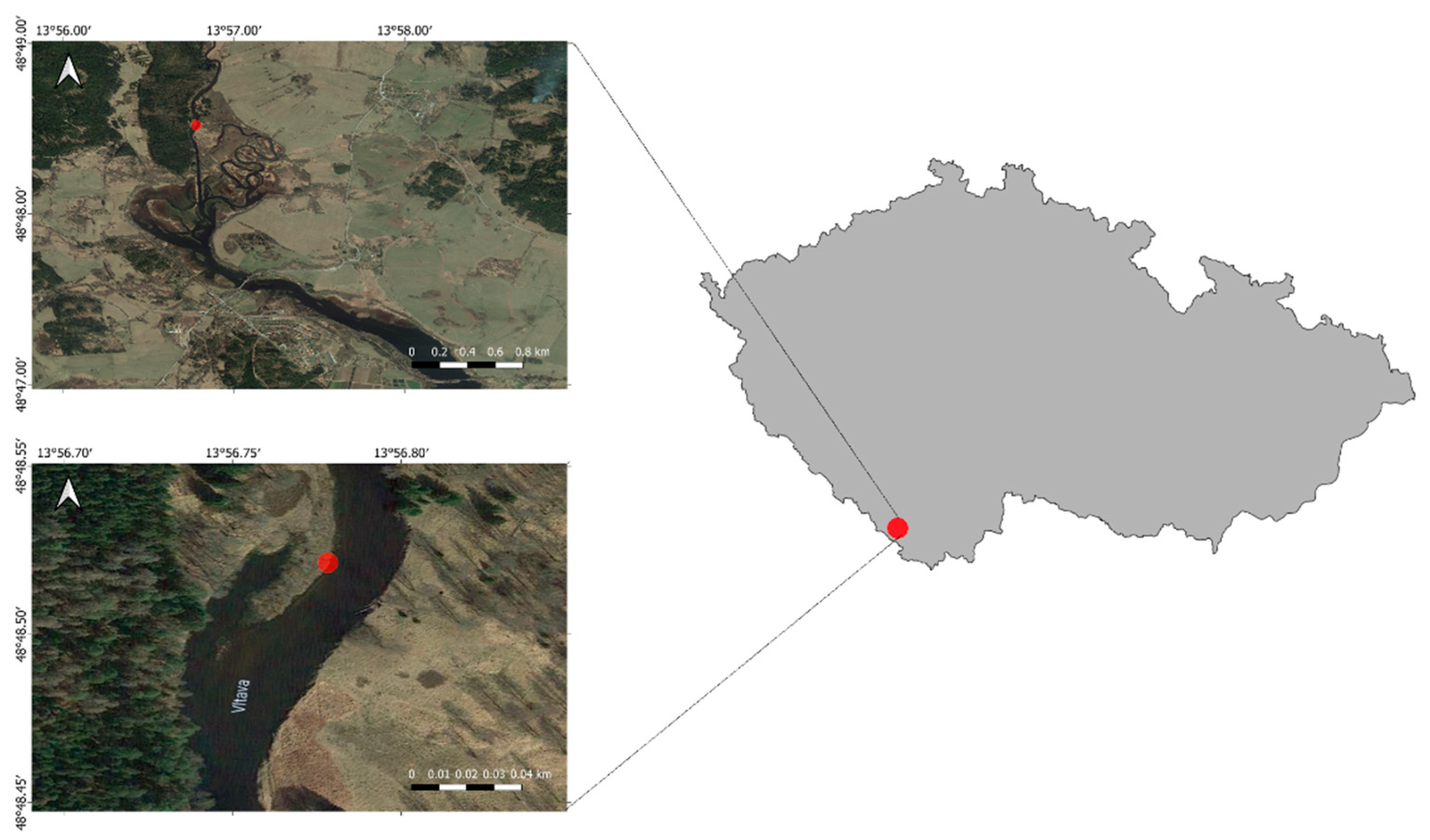
2.1. Data Collection
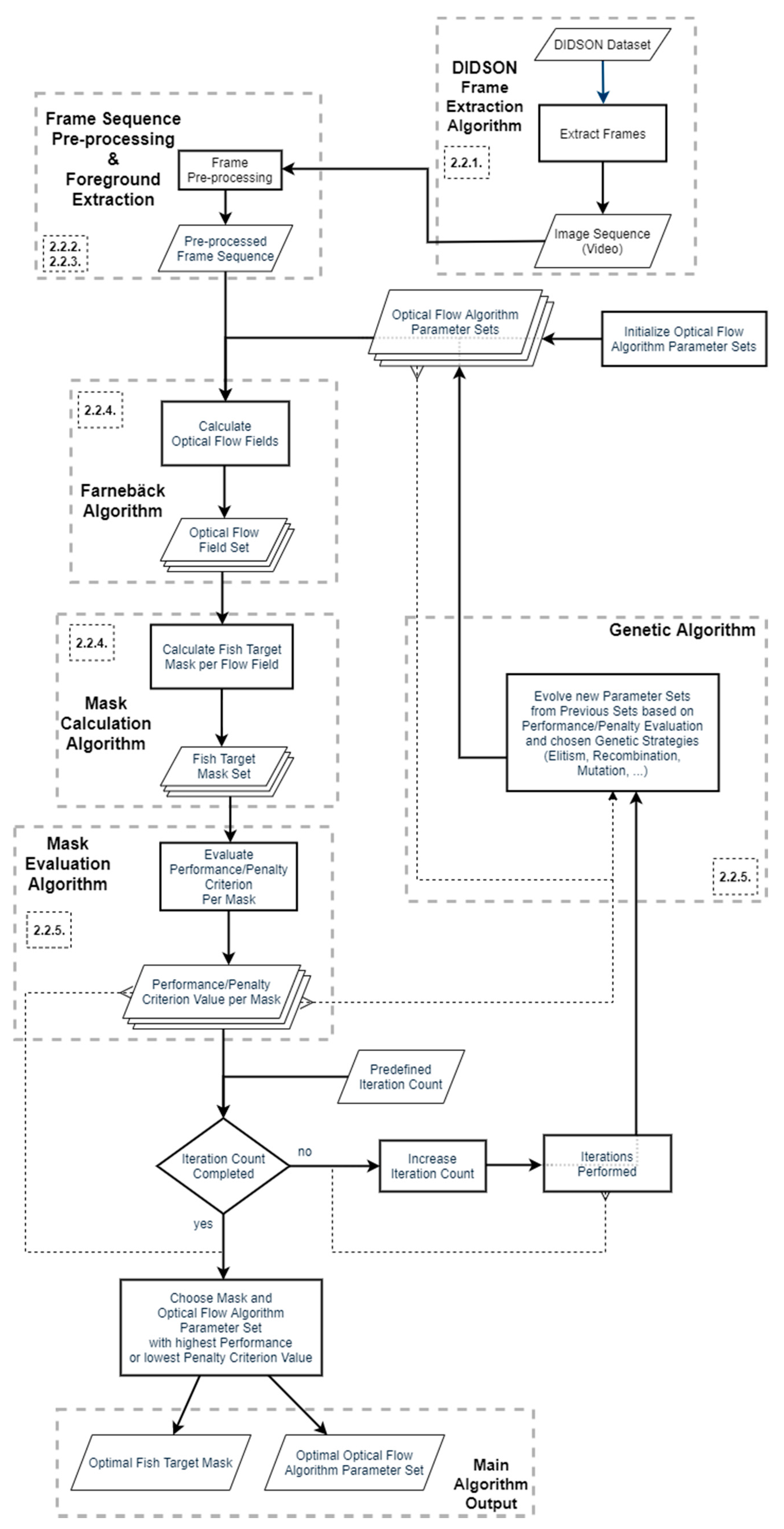
The DIDSON data were obtained from a stationary acoustic recording conducted in the Vltava River, Czech Republic [27]. A DIDSON was deployed at one site on the Vltava River in the area of the Šumava National Park (48°48.52115′ N, 13°56.77817′ E), approximately two kilometres upstream of the river mouth to the Lipno reservoir (Figure 1). In particular, a cross profile of the river was selected, where the depth was evenly increasing from the right to the left river bank, up to the deepest part, which was in the second half of the riverbed, and from where it rose again slightly towards the left bank. In addition, the riverbed at that location consisted of a finer gravel/sandy substrate, thus creating a smooth bottom surface without major obstacles. This shape of the riverbed is almost ideal for acoustic monitoring, where an acoustic device is placed in a shallower part of the riverbed, emitting a gradually expanding acoustic beam towards deeper parts of the opposite bank. In this way, almost the entire profile of the river is covered. The DIDSON acoustic beam had a cross-sectional orientation with respect to the river current, and its lower edge of the beam horizontally followed the bottom from the shallowest and deepest part of the river. Two guiding fences were used to guide fish away from the shore, where their detection by the acoustic camera would be difficult. In addition, a small fence (30–40 cm high) was placed along the bottom between the two guiding fences in order to prevent fish from passing over just above the bottom.
The data was collected in 2015, during the fish spawning period. To achieve optimal footage, the DIDSON acoustic camera was operated in the high-frequency mode (i.e., using all 96 single beams) and recorded 8 frames per second across a 10 m range (~2 cm range resolution) from 1.2 m off the camera. A 1000-frame excerpt from the footage (125 s) was used in this study.

2.2. Workflow

To extract the desired information from the DIDSON data, a multi-step procedure was designed (Figure 2), which consists of two main parts. The first part involves the fixed process of extracting and pre-processing the data with the aim of geometrically reconstructing and smoothing the frames of the raw DIDSON images, merging them into a continuous stream (video) and removing the effect of the background (Section 2.2.1, Section 2.2.2 and Section 2.2.3). The second part is an iterative process that aims to extract the optimal foreground mask, with respect to the motion that is detected in the video with the help of the optical flow, based on custom criteria for the evaluation of the output (Section 2.2.4 and Section 2.2.5). The mask extraction is achieved through the use of a genetic algorithm to detect a locally optimal parameter set for the calculation of an optical flow field to assist in the extraction of the fish target mask. The process was carried out in MATLAB® (MathWorks, Natick, MA, USA) with the use of available open-source scripts, while custom scripts were also developed as needed.

2.2.1. Data Extraction

An open-source script (ARIS Reader by Nils Olav Handegard, at https://github.com/nilsolav/ARISreader (accessed on 20 April 2019)) for MATLAB® was adapted and used to extract and geometrically reconstruct the raw DIDSON data into a video sequence that can further be analysed using computer vision algorithms and techniques. The data extraction pipeline involves parsing the raw data, converting samples to dB (decibels), building the frame-arrays and reconstructing images from the arrays through a suitable mapping from the sample space to the image (“real”) space (Figure 3).
Encoded raw data values were converted to backscattering volume SV [28], based on the instrument specifications. As the DIDSON echosounder did not apply a time-varied gain to the signals, data values were converted by applying a simple range-correction term:
S v = V r + 20 × l o g 10 r
where r represents the range, and Vr represents the recorded data value. Taking into account that r = 10 × (i/512), as 512 samples span a total range of 10 m, the expression becomes:
S v i , j = V r i , j + 20 × l o g 10 10 i 512
with (i, j) representing the row and column indices in a data sample array of a single frame recorded by a ping. Pixels outside the recorded range were padded as white.

2.2.2. Pre-processing of Reconstructed Frame Sequence

The extracted raw images were subjected to Gaussian temporal smoothing using a time window of one second (8 frames) in order to minimize the effects of noise and subsequent mis-detections. The duration of the smoothing window was chosen so as to reach a balance between a more profound smoothing effect and an adequate contrast of fish target motion in the observed speeds. Longer time windows led to a higher smoothing effect that, however, also smoothed out fish targets moving at slower speeds. Shorter time windows, on the other hand, would maintain a relatively high fish target motion contrast at the expense of potentially inadequate noise-filtering.

2.2.3. Background Subtraction—Foreground Extraction

As the instrument was stationary, the largest part of each frame did not change with time. Therefore, the background for any frame at time t was modelled through a time-lag, as the difference between each frame and the frame at a previous time, based on the predetermined time difference (tlag):
B(i,j,t) = H(i, j, t−tlag)
where B represents the background frames, and H represents the frames of the original video. The indices i and j correspond to the row and column of each pixel on the reconstructed frame (Figure 3). The foreground, F, was, therefore, calculated for each frame as:
F(i,j,t) = H(i,j,t)B(i,j,t) = H(i,j,t)H(i, j, t−tlag)
with the obvious omission of the first few frames (where t−tlag < 0). Adapting for the observed fish target motion speeds and in order to achieve adequate clarity and reliability of the resulting foreground, the time-lag was chosen to be one second of recording time (8 frames).

2.2.4. Foreground Masking using Optical Flow

Thresholding with Otsu’s method [29] was used for the segmentation of the image into foreground and background classes and the determination of the foreground mask. As this method is dependent on the degree of bimodality of the image histogram, any factor that degenerates bimodality technically limits the efficiency of this method. Typical cases are [30,31]:
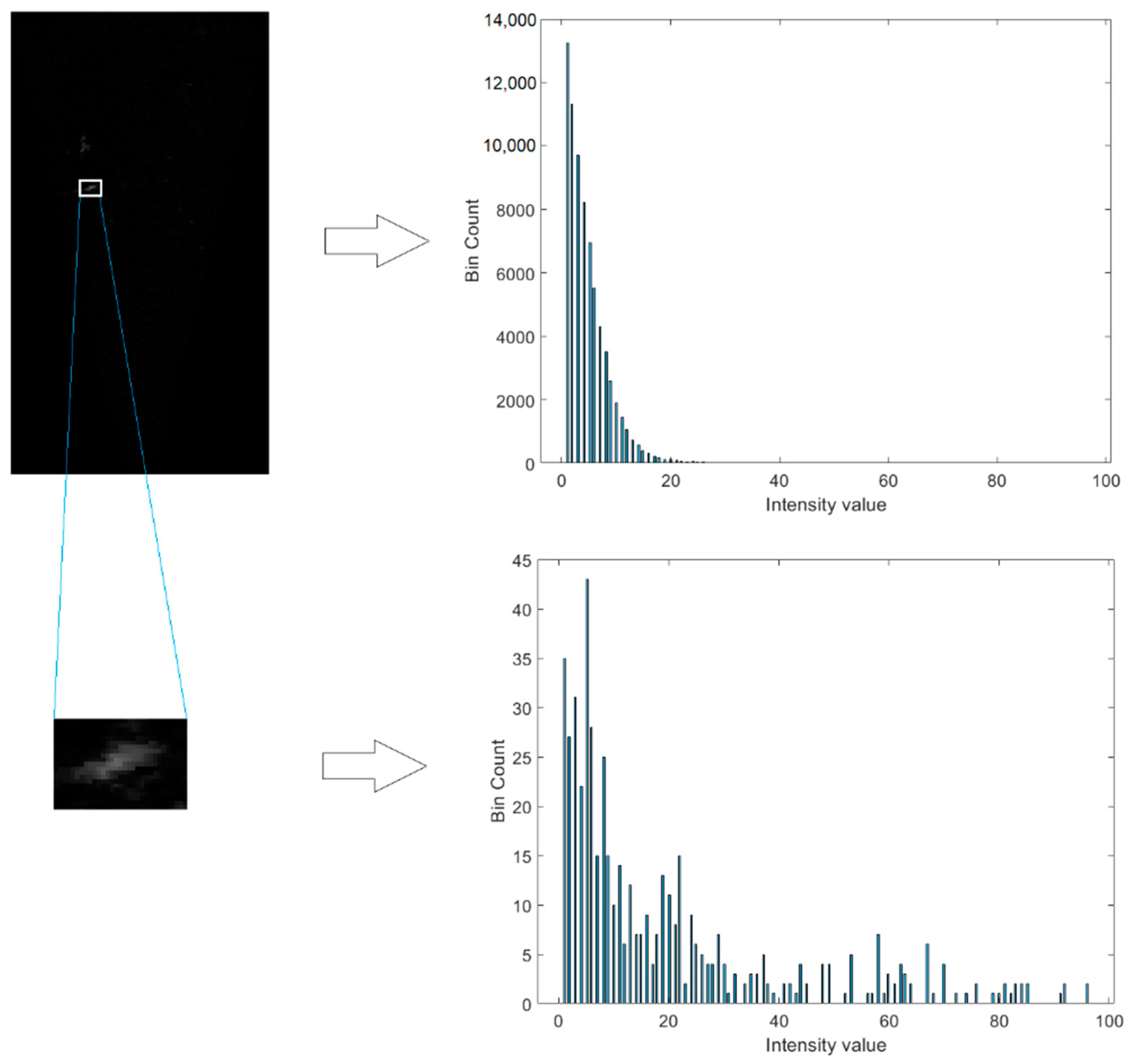
  • Imbalanced background-to-foreground pixel number ratios.
  • High variances in the foreground and background pixel values.
  • Small mean difference between foreground and background pixels.
To mitigate those problems, a large portion of the background was excluded in advance using the optical flow field of the video sequence in order to constrain the candidate fish target pixels in the close proximity of areas with detected motion. This way, the image was separated into small areas, where histogram bimodality was adequately pronounced (Figure 4). In cases like the example of Figure 4, the largest part of the frame had been attenuated through the background-removal step, with targets capturing a very small and relatively low-intensity area. Limiting the segmentation analysis in the close vicinity of the target was crucial to the successful application of Otsu’s method.
This confinement of the candidate foreground regions was based on the optical flow field of the DIDSON video sequence, using the built-in MATLAB® implementation of the Farnebäck algorithm [24]. The output of the optical flow calculation used was the velocity field, from which the velocity magnitudes (irrespective of direction) were calculated and a multi-pass thresholding method was used in order to improve the foreground mask. The multi-pass thresholding steps performed for each frame were:
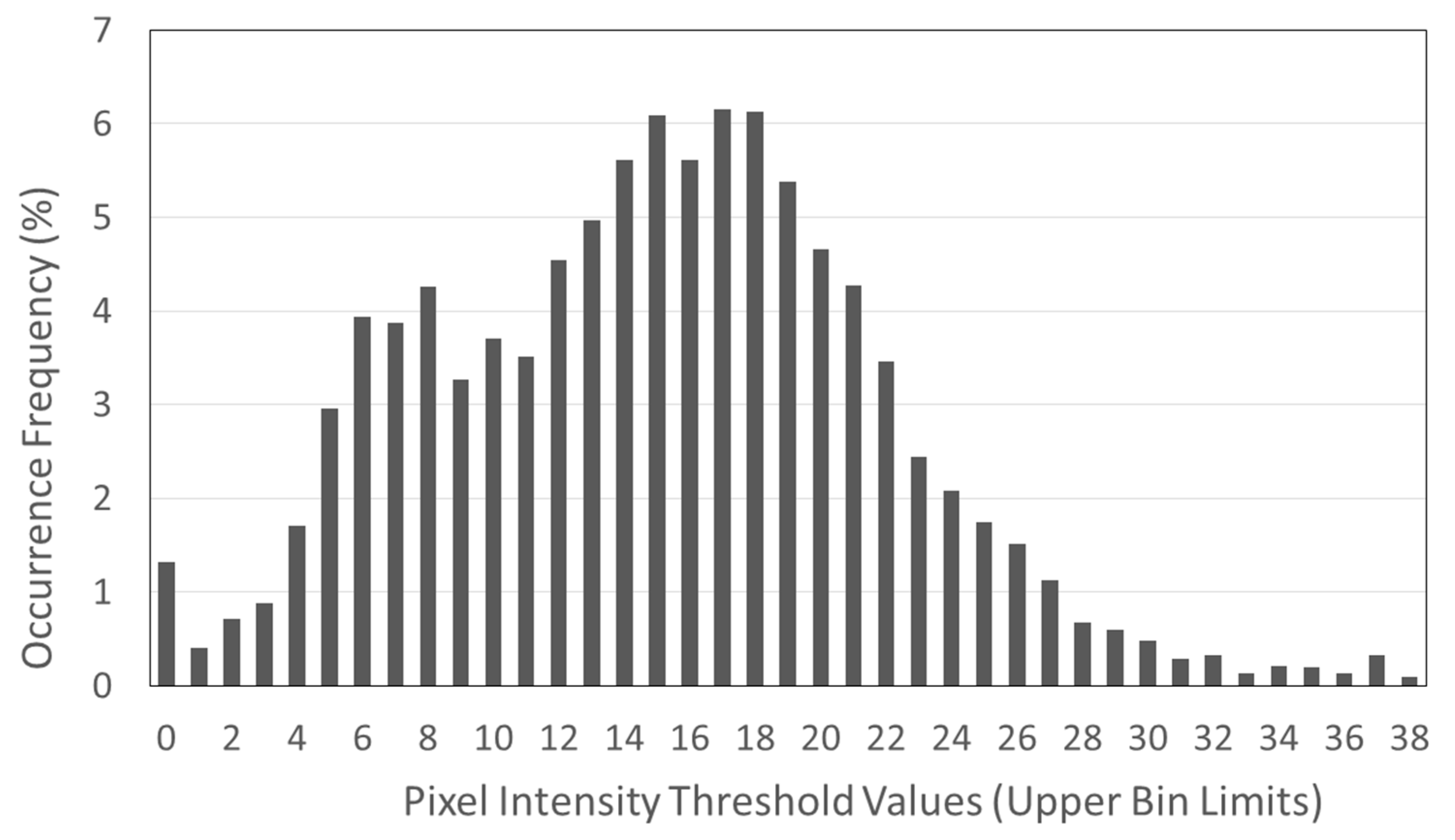
  • First threshold on the optical flow field output frame using Otsu’s method to get the optical flow mask. The background detected in this step for this frame is ignored in further calculations.
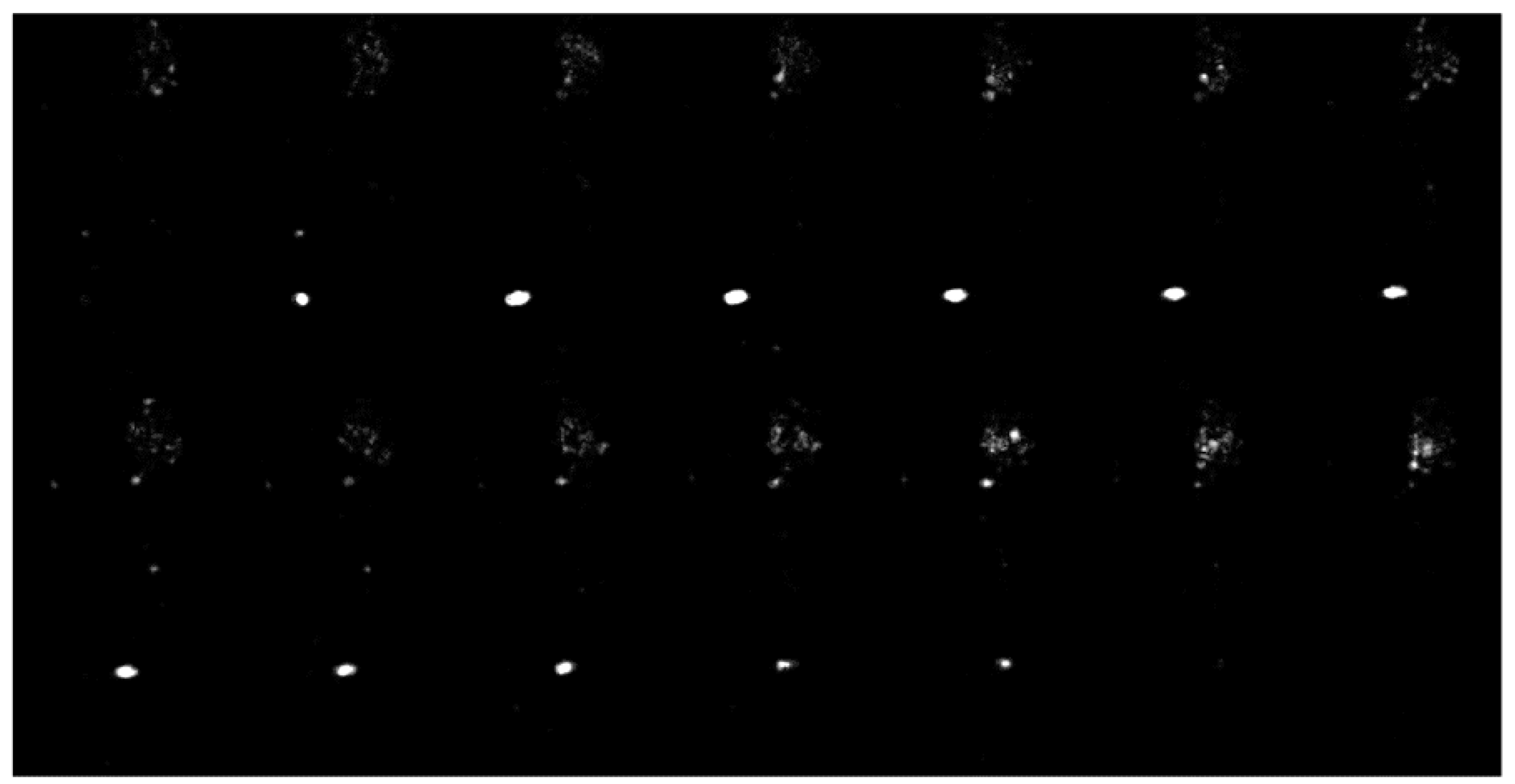
  • Detect connected components of the optical flow mask. Each component corresponds to a location of more pronounced motion on the frame.
  • For each connected component, retrieve the pixel intensity values of the original frame and perform thresholding using Otsu’s method on the component using those intensity values.
  • The final segmentation per connected component of the optical flow mask frame represents the overall fish target mask for that frame.
The calculation of the optical flow field is dependent upon the following parameters [24]:
  • The number of scales to use for the multi-scale optical flow component estimation (pyramid levels).
  • The down-sampling factor between scale levels for the scales used in the iterative calculation (pyramid scale).
  • The typical size of each neighbourhood that is polynomially approximated at each step in pixels.
  • The size of the Gaussian filter used to average displacement values estimated from different iterations in pixels.
For the application of the algorithm in the analysis, three scales were used with a down-sampling factor equal to 0.5, i.e., resolution was doubled at each level. The filter size and neighbourhood size were not specifically chosen but were instead used as parameters for optimisation using a genetic algorithm approach.

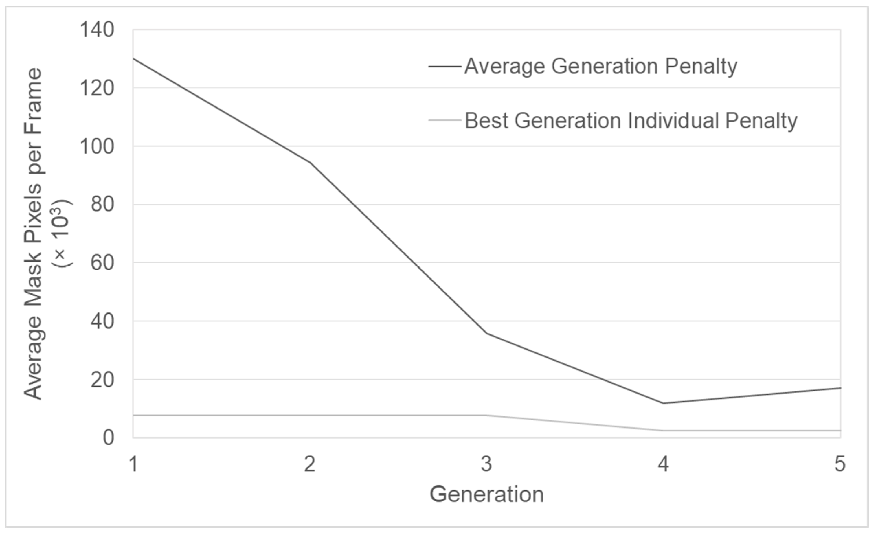
2.2.5. Genetic Algorithm—Conditionally Optimal Mask

The optical flow field calculation result is non-linearly dependent on the filter size sf, as well as the neighbourhood size sn. Optimal values for those parameters are, generally, a function of the expected target size, as well as the motion speed and directionality. As a result, their choice is usually a time-consuming iterative process. Additionally, their values are constrained to be integers in the context of image processing, as they represent image pixel units. For this reason, values for these parameters were determined by the use of a constrained genetic algorithm in MATLAB®, with a bounded solution space constrained to the integers. The following options were employed:
  • s f 3 , 70
  • s n 3 , 70
  • Population size: 6 individuals.
  • Generation limit: 5 generations.
To investigate the sensitivity of the genetic algorithm, as well as to compare the suitability of different decision criteria, two different scenarios were used to guide the algorithm, in the form of two different penalty functions:
  • Average number of masked pixels per frame.
  • Constant penalty per very small or very large object.
The first of these choices is expected to guide the genetic algorithm towards producing sf and sn parameters that lead to the tightest possible average mask per frame. The reasoning behind this choice is the minimization of the effect of large objects, such as irregularly dispersed shapes or shadows. In order to avoid convergence to unreasonably low mask pixel counts, such as empty masks, which, nevertheless, would optimize such a penalty function, a lower bound of 3 pixels was set for both the sf and the sn parameter. As the main difference of the scenarios, in terms of the output, was related to the filter and neighbourhood size parameters, the scenarios were named based on the optimal calculated parameter pair for the optical flow calculations, in the form of “sfsn”.
The reasoning behind the second choice was that the detected objects should be neither too small nor too large. This was based on observations and external knowledge of the fish target behaviour and the overall situation occurring in the location of the recordings. In specific, objects with an area < 10 px applied a penalty that is inversely proportional to their size, while objects with an area > 5000 px applied a very large constant penalty. This heuristic intended to minimize noisy detections while eliminating very large objects that would only be observed in unsuitable parameter choices or extreme processing artifacts.

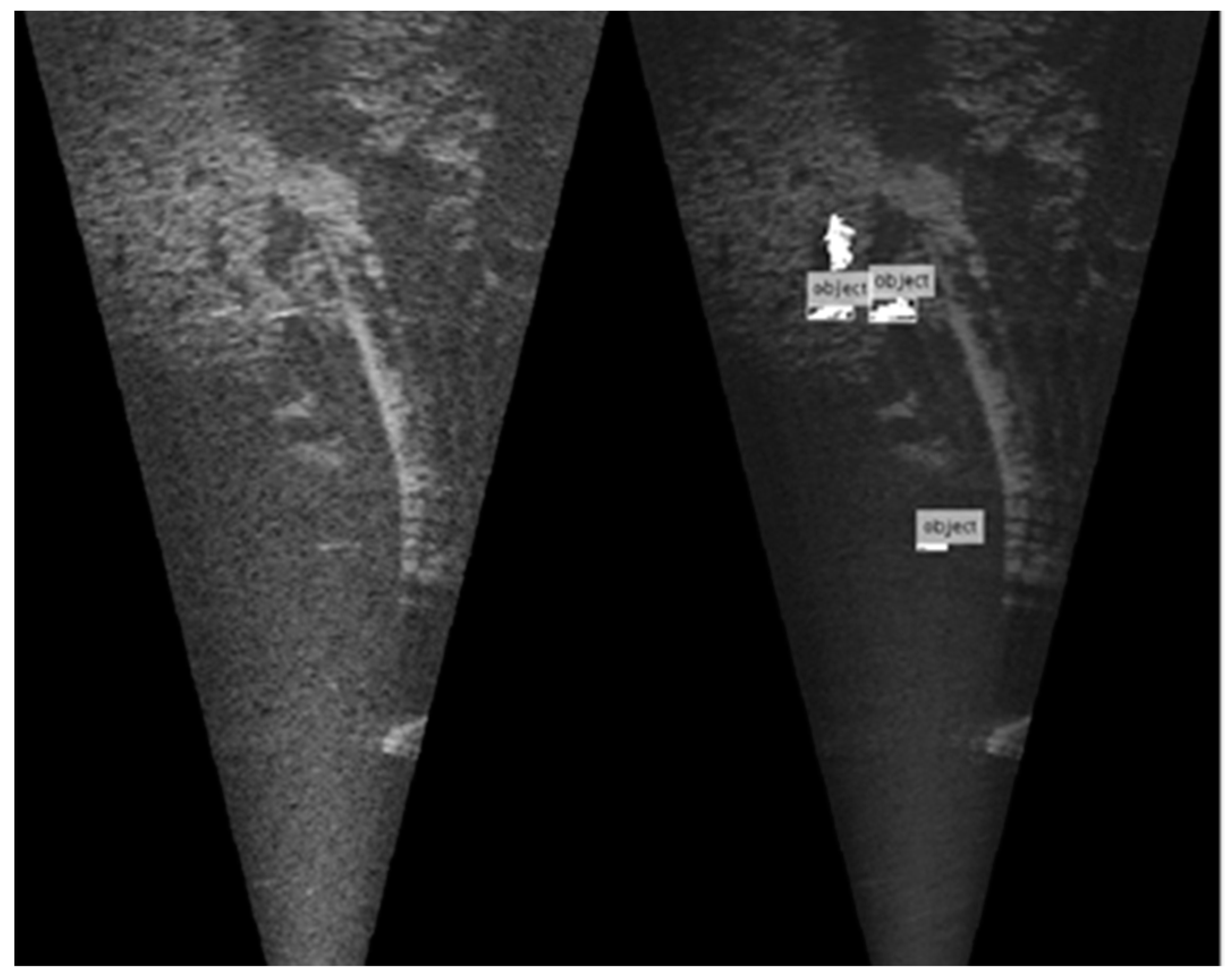
2.3. Output and Evaluation
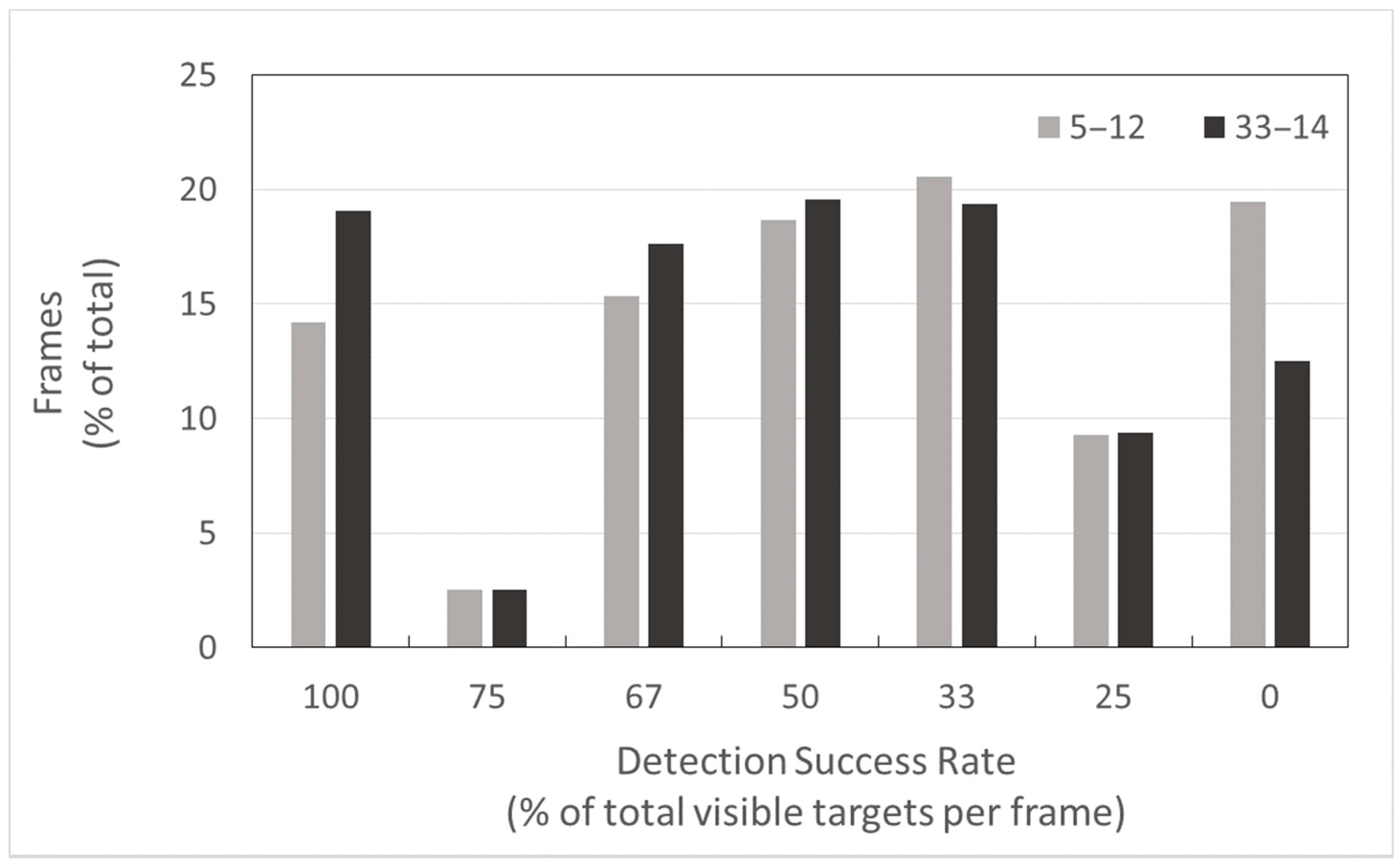
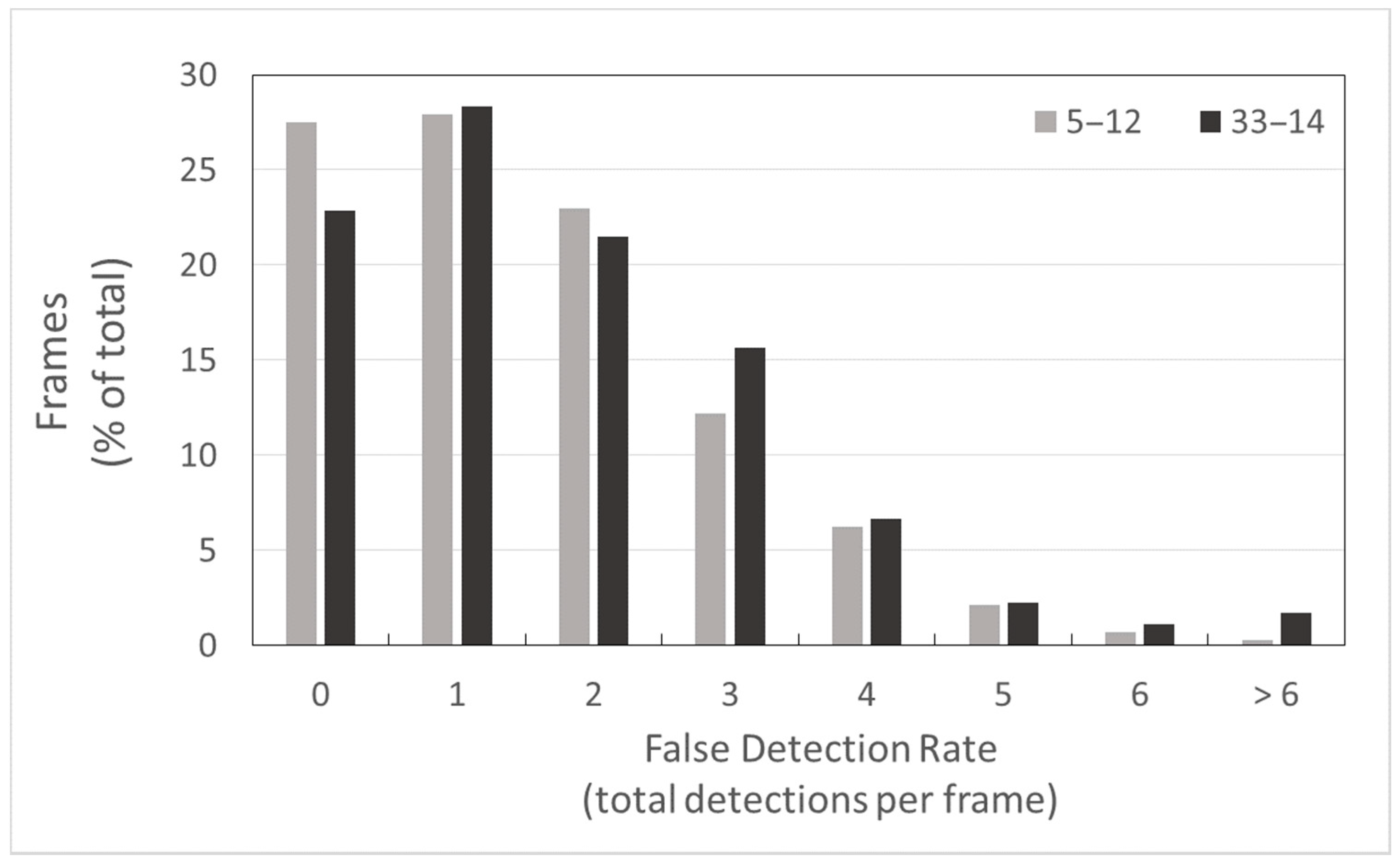
The evolution of the penalty value of the best solution of each generation determined by the genetic algorithm was plotted across generations for each scenario. The multiple automatically detected thresholds for each frame were accumulated, and their overall distribution was plotted in the form of a histogram for the optimal scenario in order to study the characteristics of the various moving targets of the video sequence. The threshold between low- and high-intensity pixels on a filtered, background-subtracted image sub-area indicates the contrast of the targets within this area against the background. Therefore, the threshold distribution can reveal information about target types, as well as give insight into the characteristics of the background. Furthermore, strips of consecutive frames were created from the resulting masks of the two scenarios, as well as from the original frames, in order to provide some insight into the nature of the analyses.
To perform a relative evaluation of the two solutions, the resulting masks were evaluated through a semi-automated target detection process, where the results were compared to those from a manual detection. Elementary automated target detection was employed for each frame, only counting targets with a total pixel area of 50 px < area < 350 px. This served as a minimum complexity baseline detection algorithm, in order to compare the performance of the two scenarios to each other by identical standards. For each scenario, a frame-pair video sequence was composed, juxtaposing the original frame, along the corresponding masked frame with the automatically detected targets. An experienced scientist observed the videos to manually detect the fish targets based on their motion across each frame. To evaluate the scenarios, each frame was assessed separately. The expert noted the number of targets correctly detected by the semi-automated process (correct detections), as well as the number of identified targets not corresponding to actual fish targets (misdetections). This way, the success rate and false detections were measured and compared between the two scenarios. The percentage of frames for each distinct detection success rate (percentage of correct targets included in the mask) and false detection rate (percentage of targets incorrectly included in the mask).

3. Results

The evolution of the penalty decreased within the evolutionary progression of 5 consecutive generations in both the first (average mask pixels per frame as the total penalty, Figure 5) as well as the second scenario (constant penalty applied to targets > 5000 px and a size-dependent penalty applied to targets < 10 px, Figure 6). The genetic algorithm was successful in significantly optimising the corresponding purpose of each scenario by minimising the assigned penalty function. The optical flow parameters determined for scenario 1 were sf = 5, sn = 12, whence it was named 5–12, while for scenario 2, the determined optimal parameter values were sf = 33, sn = 14, whence it was named 33–14.
The difference threshold histogram for the optimal solution of scenarios 33–14 was approximately bimodal and revealed two peaks at pixel intensity difference values of approximately 8 and 18. The distribution of thresholds for areas with optical-flow-detected motion was scattered, with a significant drop in pixel intensity difference threshold values of approximately 25 and above, as well as below 4. The two peaks indicate the existence of a group of targets that have a relatively higher contrast to the background (higher difference threshold), as well as a group of targets that have a lower contrast to the background (Figure 7). The calculated threshold values correspond to Otsu’s segmentation thresholds of intensity distributions within the areas roughly identified as motion by the optical flow. Since the pixel intensities have undergone smoothing and background subtraction, these threshold values are directly representational of the target residual signal strength and, consequently, its discernibility, with a perfect zero almost definitively indicating the background.
One interpretation of the lower threshold values is their correspondence to lower reliability of detection, whereby the specific targets are considered as borderline foreground or, potentially, present the character of occasional occlusions of the background. Another interpretation might lie within the assumption that the detected targets exhibit variability in their acoustic characteristics, with some species producing stronger backscatter than others, with this observation manifesting into the relatively wide observed range of possible thresholds with respect to the proximal background of each target. In the case of the present study, the specific recording layout and the relative shallowness of the river, the lower-contrast targets, represented by the histogram region close to and around the lower peak, are most likely the detections of fish target shadows. Those are reflected on the river bottom and bank areas, which generally consist of lower pixel intensities after background subtraction, thereby producing the moving background occlusion patterns that present as lower intensity targets. The assumption of variable acoustic characteristics manifesting as correspondingly variable target-to-background segmentation thresholds remains valid but cannot adequately account for the wide range of observed thresholds. The most likely explanation for the wide range is the strong interference of the background onto the targets due to the recording layout and situation, whereby the relatively small distances of the targets from the riverbed lead to varying target contrasts throughout the analysed frame sequence.
Generally, the optical flow-determined magnitudes provided more diffuse motion-sensitive masking (Figure 8), while the subsequent adaptive thresholding served to clarify and intensify the edges between actual targets and the background (Figure 9). Additionally, the finally calculated mask provided relatively decent segmentation between moving targets and background for the optimized parameter choices, while execution of the optical flow-based mask extraction algorithm (excluding the genetic-algorithm-driven penalty-based optimization) using a randomly selected test input parameter set of sf = 25 and sn = 30 provided a result containing many highly noisy mask frames, thereby highlighting the sensitivity of the masking process to the optical flow input parameters (Figure 10).
A special layout for the manual detection and evaluation was used to assess the performance of the optimal solution for each of the two scenarios (Figure 11) under the elementary detection process outlined in 2.3 (i.e., detections of 50 px < area < 350 px). The percentage of match between manually and automatically detected fish targets (i.e., detection success rate) was calculated for each frame and frames were grouped per success rate. Scenario 33–14 outperformed scenario 5–12 with a higher percentage of perfectly (100% success rate) detected frames, i.e., 19% for scenario 33–14 vs. ~14% for scenario 5–12. At the same time, scenario 33–14 also exhibited fewer totally missed frames (0% success rate) with 12.5% for scenario 33–14 vs. ~19.5% for scenario 5–12. False detection rates were also recorded for each frame in terms of absolute numbers, and frames were, again, grouped by false detection counts. Scenario 33-14 exhibited slightly higher false detection rates, with fewer than 23% perfect frames (0 false detections) vs. 27.5% for scenario 5–12. Both scenarios, however, exhibited at least 50% of the frames with at most a single falsely detected target. Overall, in 22.3% of the total analysed frames, the 33–14 scenario outperformed the 5–12 scenario with a higher success rate (more correct detections), while the opposite was true in 11.8% of the frames. The correct detections were identical in the largest part of the analysed frames, namely 65.9% (Figure 12 and Figure 13, Table 1).

4. Discussion

Machine learning techniques have been widely used to tackle both water resource management problems [32,33] as well as fisheries management problems [34]. However, there is limited literature regarding the use of these techniques in data mining from certain types of datasets, such as DIDSON recordings. Fuzziness in the data, minimum and maximum expected target size, average single-target shape and average target separation distance are, among others, just a few of the variables that can affect the capability of algorithms to detect and track single targets throughout a DIDSON dataset [19,21,35]. This study introduces a novel approach to the automatic classification of fish targets in DIDSON recordings, which minimises human intervention. The algorithm combines tools from the fields of machine learning and computer vision with more widely used image processing and segmentation techniques with the aim of conditionally optimising the characteristics of the resulting foreground mask.
An exploratory application of the proposed workflow in a specific sample exhibited promising results for the masking of moving targets. The threshold value distribution indicated a wide variety of target-to-background contrasts, demonstrating the ability of the algorithm to detect objects of heterogeneous visual characteristics in the reconstructed video sequence (hence, acoustic characteristics in the original recordings), even within the same frame. Identifying the most frequent contrast thresholds and the corresponding target groups may be vital in determining a single threshold or a cut-off contrast threshold value for the exclusion of undesired masked objects such as, in the context of this study, reflections of fish target shadows on the background (river bottom and bank). An elementary automated object detection algorithm also revealed relatively high success rates, while the level of observed missed and false detection rates should not be unmanageable for relatively sophisticated state-of-the-art tracking algorithms to fill the gaps.
Regarding the sensitivity of the workflow to the input parameters, the filter size (sf) and the neighbourhood size (sn), both used for the calculation of the optical flow field from the DIDSON image sequence, were confirmed to significantly affect the finally calculated mask. A (sf—sn) choice of (5–12) was shown to conditionally minimise the total masked pixels for each frame, while a choice of (33–14) conditionally minimised the total number of very small or very large discrete connected components (targets). The overall algorithm strongly depends on an efficient formulation of a penalty function. While being one of the strong points of the proposed methodology, as it allows the researchers to freely express the intended criteria in terms of the result, a proper formulation of the penalty function is not always intuitive. Additionally, it often needs to reflect intelligent criteria in a deterministic manner, which sometimes further complicates things.
Data mining from large datasets is intimately tied to the nature of the knowledge to be extracted, i.e., the specific patterns to be discovered. Fayyad et al. [36] define a pattern as “an expression in some language describing a subset of the data or a model applicable to the subset.” A pattern may not always be possible to search for without accordingly sophisticated tools. As an example, tools for image segmentation aimed at single-frame target detection cannot utilize information from preceding or following frames in case the target is known to be moving across frames. Thus, expressing existing (potentially empirical) knowledge into a pattern recognition algorithm in order to improve solutions depends on the flexibility of the definition, as well as the algorithm itself. Deterministic tools are easier to understand and use but offer less flexibility in integrating specialised knowledge about the problem. While automatic thresholding techniques, such as Otsu’s method, involve single frames, the optical flow inherently integrates the understanding of patterns such as cross-frame target displacement, effectively incorporating this knowledge into the solutions. Furthermore, its parameters express more intuitive, higher-level concepts, such as the neighbourhood size, which refers to a sliding sub-window within an image, whereinto assess for overall target motion. Perhaps more importantly, a genetic algorithm offers the flexibility of a fully customisable pattern, expressed in a mathematical form in terms of the expected result, which the algorithm then works to indiscriminately minimise or maximise.
An important family of computational techniques, collectively identified with the term soft computing [37], specifically as opposed to hard computing (i.e., using precisely defined calculations), provides a paradigm with the potential of tackling problems, such as that of target identification and tracking from fuzzy input. This paradigm embraces limitations inherent to the problem definitions, such as, among others, imprecision, data holes or fuzziness and approximations [38]. The field of soft computing has recently resurfaced into the spotlight of scientific research, following the technological advances and breakthroughs of the last few decades, which have allowed easier access to implementation tools and resources [38]. Various studies already published in other fields, such as [39], have already demonstrated the feasibility and benefits of soft computing techniques in real-world applications. In this context, the present study can also be considered an attempt to model the problem of motion detection and target identification and tracking in DIDSON data without circumventing its imprecisely defined elements and devise a way to tackle it with soft computing methodologies.
The most important point of this study was the demonstration of the synergy between deterministic mathematical tools, higher-level machine learning and computer vision techniques, as well as expert knowledge, in order to tackle a complicated problem in the field of fisheries acoustics. Modelling the problem as a statement can probably best demonstrate how the tools were employed to build a consistent workflow. Therefore, the problem of detecting targets motivated the distinction between a foreground (moving targets) and a background, which was tackled through thresholding. The knowledge that these targets are moving on a video was the motivation for employing the optical flow. The expert knowledge that those targets may have different acoustic characteristics and may, consequently, have different visual characteristics on the reconstructed video sequence was the motivating factor behind the choice of adaptive piecewise thresholding, combined with the optical flow. Finally, the piece of knowledge regarding the fact that too small or too large targets most often represent noisy detections was integrated into the algorithm through a penalty function to be minimised by an appropriately set-up genetic algorithm.
The effect of the penalty function on the convergence of the genetic algorithm to an optimal solution is also reflected in the calculations used in the study. According to the employed optical flow algorithm [24], larger filter sizes make motion detection more blurred but also more robust to noise. The penalty function of the second scenario was expressed, in part, in a way that penalises the detection of very small objects. Based on expert knowledge, very small detections are, effectively, interpreted as noisy results; therefore, the penalty function was an indirect expression aimed at minimising what would be considered as noise. As a result, the genetic algorithm, in turn, converged to a solution that minimises this formulation by employing a larger filter size, which is known to make flow determination more robust to noise by smoothing the motion magnitudes over each neighbourhood. This observation serves to highlight the translation of knowledge through the penalty function into the finally determined solution.
A test run of the algorithm on a sequence of 4000 frames of the original recordings, reconstructed to a 717 × 400 px video was also conducted to acquire insight into its computational complexity. A complete single-threaded (no parallel execution) run of the main algorithm on this dataset took approximately 5 h on a Windows 10 System with an Intel® Core™ i7-9750H (2.6 GHz) processor (Intel Corporation, Santa Clara, California, U.S.) and 32GB of available RAM. This highlights the necessity for potential implementation of specific improvements, especially the parallelization of the applied algorithm, which could lead to multiple reductions in run-time, especially in the light of modern multi-core processor availability.
Fish target detection on a recorded video, regardless of the original source, is usually relatively easy to perform by plain visual review. However, not all visually contributing parameters can be integrated into an automated pattern recognition algorithm for target classification. Potential improvements to most typical workflows could be based on the combination of empirical observations, as well as a better knowledge of fish behavioural patterns [22]. Further work could be carried out in order to improve the quality of the output of the proposed algorithm or fine-tune its workflow by assessing its performance on a different dataset, which would include different fish stock compositions, signal-to-noise ratios and exposure to different environmental factors. Missed detections can always be minimised through the use of suitable tracking methodologies, while the employed machine learning and computer vision techniques could be further extended to encompass steps involved in the tracking techniques as well. Since a number of specialised software packages for the processing of DIDSON datasets already exist, which offer customised tools for target detection and tracking, the proposed methodology could be combined with such packages for the integrated processing of DIDSON recordings. Naturally, any potential adoption of the proposed algorithmic techniques, or variations thereof, would have to be preceded by extensive validation on multiple diverse dataset samples, possibly under a suitable formal evaluation framework.

Author Contributions

Conceptualization, T.-M.P., M.T., D.T. and S.P.S.; Data curation, T.-M.P., M.T. and D.T.; Formal analysis, T.-M.P. and D.T.; Funding acquisition, M.T.; Investigation, T.-M.P. and D.T.; Methodology, T.-M.P., D.T. and S.P.S.; Resources, M.T.; Software, T.-M.P., M.T. and D.T.; Supervision, M.T., S.P.S. and I.A.; Validation, M.T.; Visualization, T.-M.P. and D.T.; Writing—original draft, T.-M.P.; Writing—review & editing, M.T., D.T., S.P.S. and I.A. All authors have read and agreed to the published version of the manuscript.

Funding

This research received no external funding.

Institutional Review Board Statement

Not applicable.

Informed Consent Statement

Not applicable.

Data Availability Statement

The data used in this study are available upon request, from the corresponding author.

Acknowledgments

The DIDSON dataset used in the study was acquired from the project “Coexistence of human and the pearl mussel Margaritifera margaritifera in the Vltava River floodplain,” funded by The Operational Programme Environment in 2014–2015.

Conflicts of Interest

The authors declare no conflict of interest.

References

  1. Bizzi, S.; Demarchi, L.; Grabowski, R.C.; Weissteiner, C.J.; Van de Bund, W. The Use of Remote Sensing to Characterise Hydromorphological Properties of European Rivers. Aquat. Sci. 2016, 78, 57–70. [Google Scholar] [CrossRef] [Green Version]
  2. Bhat, S.U.; Pandit, A.K. Water Quality Assessment and Monitoring of Kashmir Himalayan Freshwater Springs-A Case Study. Aquat. Ecosyst. Heal. Manag. 2020, 23, 274–287. [Google Scholar] [CrossRef]
  3. Domakinis, C.; Mouratidis, A.; Voudouris, K.; Astaras, T.; Karypidou, M.C. Flood Susceptibility Mapping in Erythropotamos River Basin with the Aid of Remote Sensing and GIS. AUC Geogr. 2020, 55, 149–164. [Google Scholar] [CrossRef]
  4. Mouratidis, A.; Sarti, F. Flash-Flood Monitoring and Damage Assessment with SAR Data: Issues and Future Challenges for Earth Observation from Space Sustained by Case Studies from the Balkans and Eastern Europe. Lect. Notes Geoinf. Cart. 2013, 199659, 125–136. [Google Scholar] [CrossRef]
  5. Palmer, M.A.; Bernhardt, E.S.; Allan, J.D.; Lake, P.S.; Alexander, G.; Brooks, S.; Carr, J.; Clayton, S.; Dahm, C.N.; Follstad Shah, J.; et al. Standards for Ecologically Successful River Restoration. J. Appl. Ecol. 2005, 42, 208–217. [Google Scholar] [CrossRef]
  6. Karr, J. Biological Integrity: A Long-Neglected Aspect of Water Resource Management. Ecol. Soc. Am. Ecol. Appl. 1991, 1, 66–84. [Google Scholar] [CrossRef] [PubMed]
  7. Simmonds, E.J.; MacLennan, D. Fisheries Acoustics: Theory and Practice, 2nd ed.; Blackwell Publishing: Hoboken, NJ, USA, 2005. [Google Scholar] [CrossRef]
  8. Foote, K.G. Acoustic Methods: Brief Review and Prospects for Advancing Fisheries Research. In The Future of Fisheries Science in North America; Beamish, R.J., Rothschild, B.J., Eds.; Springer: Dordrecht, The Netherlands, 2009; pp. 313–343. [Google Scholar] [CrossRef]
  9. Moursund, R.A.; Carlson, T.J.; Peters, R.D. A Fisheries Application of a Dual-Frequency Identification Sonar Acoustic Camera. ICES J. Mar. Sci. 2003, 60, 678–683. [Google Scholar] [CrossRef]
  10. Belcher, E.; Matsuyama, B.; Trimble, G. Object Identification with Acoustic Lenses. In TS/IEEE Oceans 2001. An Ocean Odyssey. Conference Proceedings (IEEE Cat. No.01CH37295), Honolulu, HI, USA, 5–8 November 2001; IEEE: Piscataway, NJ, USA, 2001; Volume 1, pp. 6–11. [Google Scholar] [CrossRef]
  11. Belcher, E.; Hanot, W.; Burch, J. Dual-Frequency Identification Sonar (DIDSON). In Proceedings of the 2002 International Symposium on Underwater Technology (Cat. No.02EX556), Tokyo, Japan, 19 April 2002; IEEE: Piscataway, NJ, USA, 2002; pp. 187–192. [Google Scholar] [CrossRef]
  12. Sound Metrics. Available online: www.soundmetrics.com (accessed on 17 December 2019).
  13. Pipal, K.; Jessop, M.; Boughton, D.; Adams, P. Using Dual-Frequency Identification Sonar (DIDSON) to Estimate Adult Steelhead Escapement in the San Lorenzo River, California. Calif. Fish Game 2010, 96, 90–95. [Google Scholar]
  14. Faulkner, A.V.; Maxwell, S.L. An Aiming Protocol for Fish-Counting Sonars Using River Bottom Profiles from a Dual-Frequency Identification Sonar (DIDSON); Alaska Department of Fish and Game, Division of Sport Fish, Research and Technical Services: Juneau, AK, USA, 2009. [Google Scholar]
  15. Burwen, D.L.; Fleischman, S.J.; Miller, J.D. Accuracy and Precision of Salmon Length Estimates Taken from DIDSON Sonar Images. Trans. Am. Fish. Soc. 2010, 139, 1306–1314. [Google Scholar] [CrossRef]
  16. Daroux, A.; Martignac, F.; Nevoux, M.; Baglinière, J.L.; Ombredane, D.; Guillard, J. Manual Fish Length Measurement Accuracy for Adult River Fish Using an Acoustic Camera (DIDSON). J. Fish Biol. 2019, 95, 480–489. [Google Scholar] [CrossRef] [PubMed]
  17. van Keeken, O.A.; van Hal, R.; Volken Winter, H.; Tulp, I.; Griffioen, A.B. Behavioural Responses of Eel (Anguilla Anguilla) Approaching a Large Pumping Station with Trash Rack Using an Acoustic Camera (DIDSON). Fish. Manag. Ecol. 2020, 27, 464–471. [Google Scholar] [CrossRef] [Green Version]
  18. Rakowitz, G.; Tušer, M.; Říha, M.; Jůza, T.; Balk, H.; Kubečka, J. Use of High-Frequency Imaging Sonar (DIDSON) to Observe Fish Behaviour towards a Surface Trawl. Fish. Res. 2012, 123–124, 37–48. [Google Scholar] [CrossRef]
  19. Martignac, F.; Daroux, A.; Bagliniere, J.L.; Ombredane, D.; Guillard, J. The Use of Acoustic Cameras in Shallow Waters: New Hydroacoustic Tools for Monitoring Migratory Fish Population. A Review of DIDSON Technology. Fish Fish. 2015, 16, 486–510. [Google Scholar] [CrossRef]
  20. Lenihan, E.S.; McCarthy, T.K.; Lawton, C. Use of an Acoustic Camera to Monitor Seaward Migrating Silver-Phase Eels (Anguilla Anguilla) in a Regulated River. Ecohydrol. Hydrobiol. 2019, 19, 289–295. [Google Scholar] [CrossRef]
  21. Langkau, M.C.; Balk, H.; Schmidt, M.B.; Borcherding, J. Can Acoustic Shadows Identify Fish Species? A Novel Application of Imaging Sonar Data. Fish. Manag. Ecol. 2012, 19, 313–322. [Google Scholar] [CrossRef]
  22. Mueller, A.-M.; Mulligan, T.; Withler, P.K. Classifying Sonar Images: Can a Computer-Driven Process Identify Eels? North Am. J. Fish. Manag. 2008, 28, 1876–1886. [Google Scholar] [CrossRef] [Green Version]
  23. Han, J.; Honda, N.; Asada, A.; Shibata, K. Automated Acoustic Method for Counting and Sizing Farmed Fish during Transfer Using DIDSON. Fish. Sci. 2009, 75, 1359–1367. [Google Scholar] [CrossRef]
  24. Farnebäck, G. Two-Frame Motion Estimation Based On. Lect. Notes Comput. Sci. 2003, 2749, 363–370. [Google Scholar]
  25. Solichin, A.; Harjoko, A.; Putra, A.E. Movement Direction Estimation on Video Using Optical Flow Analysis on Multiple Frames. Int. J. Adv. Comput. Sci. Appl. 2018, 9, 174–181. [Google Scholar] [CrossRef]
  26. Bhanu, B.; Lee, S.; Ming, J. Adaptive Image Segmentation Using a Genetic Algorithm. IEEE Trans. Syst. ManCybern. 1995, 25, 1543–1567. [Google Scholar] [CrossRef]
  27. Muška, M.; Tušer, M. Soužití Člověka a Perlorodky Říční ve Vltavském Luhu: G—Monitoring Populací Ryb ve Vltavě, Kvantifikace Migrace Ryb z Přehrady Lipno Do Toku Vltavy [Coexistence of Human and the Pearl Mussel Margaritifera Margaritifera in the Vltava River Floodplain, G.; Biologické centrum, v.v.i., Hydrobiologický ústav: České Budějovice, Czech Republic, 2015. [Google Scholar]
  28. Maclennan, D.N.; Fernandes, P.G.; Dalen, J. A Consistent Approach to Definitions and Symbols in Fisheries Acoustics. Ices J. Mar. Sci. 2002, 59, 365–369. [Google Scholar] [CrossRef] [Green Version]
  29. Otsu, N. A Threshold Selection Method from Gray-Level Histograms. IEEE Trans. Syst. Man. Cybern. 1979, 9, 62–66. [Google Scholar] [CrossRef] [Green Version]
  30. Lee, S.U.; Yoon Chung, S.; Park, R.H. A Comparative Performance Study of Several Global Thresholding Techniques for Segmentation. Comput. Vis. Graph. Image Process. 1990, 52, 171–190. [Google Scholar] [CrossRef]
  31. Kittler, J.; Illingworth, J. On Threshold Selection Using Clustering Criteria. IEEE Trans. Syst. Man. Cybern. 1985, SMC-15, 652–655. [Google Scholar] [CrossRef]
  32. Sentas, A.; Psilovikos, A.; Karamoutsou, L.; Charizopoulos, N. Monitoring, Modeling, and Assessment of Water Quality and Quantity in River Pinios, Using ARIMA Models. Desalin. Water Treat. 2018, 133, 336–347. [Google Scholar] [CrossRef]
  33. Sentas, A.; Karamoutsou, L.; Charizopoulos, N.; Psilovikos, T.; Psilovikos, A.; Loukas, A. The Use of Stochastic Models for Short-Term Prediction of Water Parameters of the Thesaurus Dam, River Nestos, Greece. Proceedings 2018, 2, 634. [Google Scholar] [CrossRef] [Green Version]
  34. Suryanarayana, I.; Braibanti, A.; Sambasiva Rao, R.; Ramam, V.A.; Sudarsan, D.; Nageswara Rao, G. Neural Networks in Fisheries Research. Fish. Res. 2008, 92, 115–139. [Google Scholar] [CrossRef]
  35. Tušer, M.; Frouzová, J.; Balk, H.; Muška, M.; Mrkvička, T.; Kubečka, J. Evaluation of potential bias in observing fish with a DIDSON acoustic camera. Fish. Res. 2014, 155, 114–121. [Google Scholar] [CrossRef]
  36. Fayyad, U.; Piatetsky-Shapiro, G.; Smyth, P. From Data Mining to Knowledge Discovery in Databases. AI Mag. 1996, 17, 37. [Google Scholar] [CrossRef]
  37. Zadeh, L. Fuzzy Logic, Neural Networks and Soft Computing. Comm. ACM 1994, 37, 77–84. [Google Scholar] [CrossRef]
  38. Dogan, I. An Overview of Soft Computing. Proc. Comp. Sci. 2016, 102, 34–38. [Google Scholar] [CrossRef] [Green Version]
  39. Ghalandari, M.; Ziamolki, A.; Mosavi, A.; Shamshirband, S.; Chau, K.-W.; Bornassi, S. Aeromechanical optimization of first row compressor test stand blades using a hybrid machine learning model of genetic algorithm, artificial neural networks and design of experiments. Eng. App. Comp. Fl. Mech. 2019, 13, 892–904. [Google Scholar] [CrossRef]
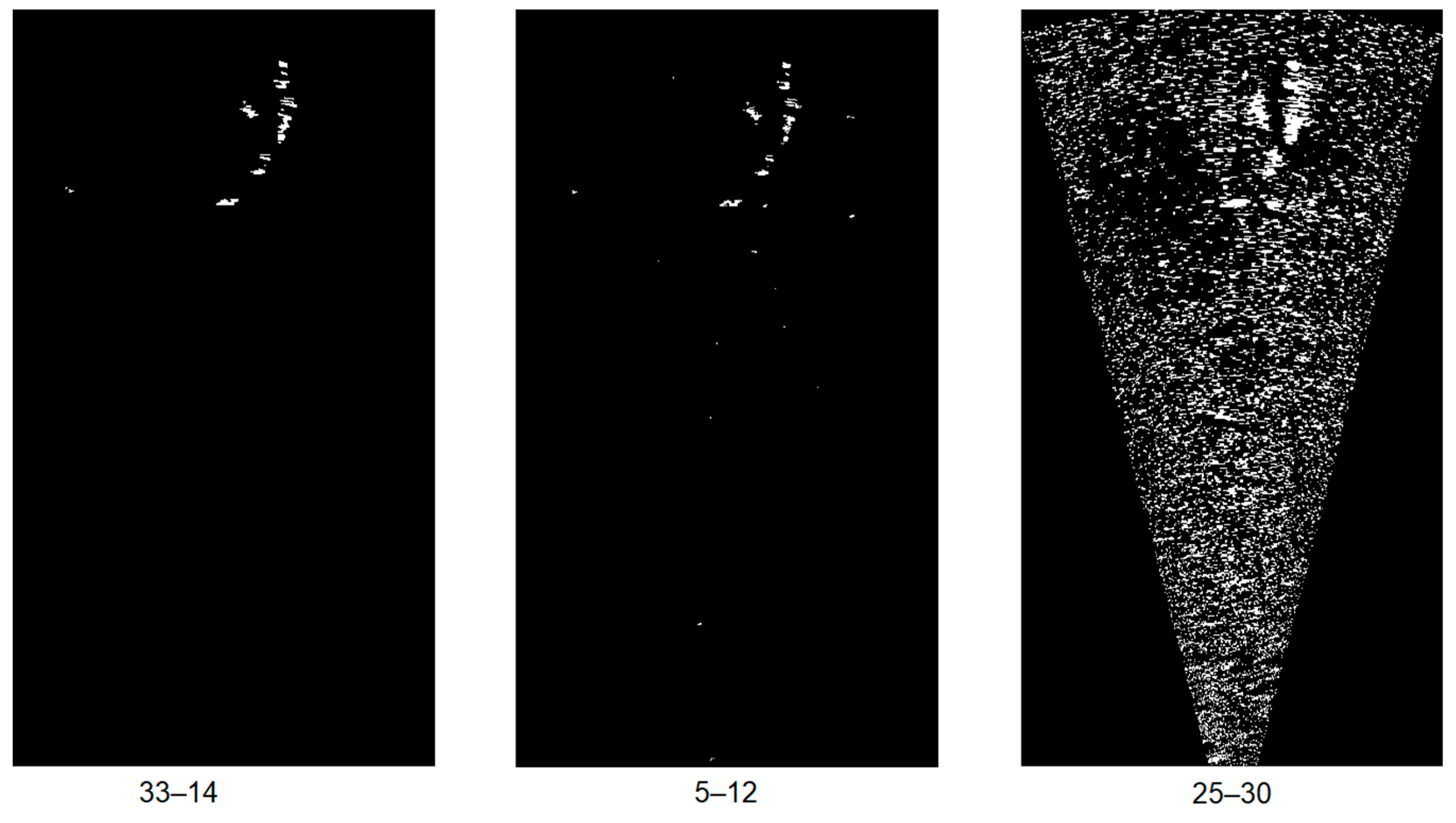
 [Green Version]
Figure 1. The site studied for monitoring fish upstream migration was located on the Vltava River, Czech Republic, approximately 2 km upstream off the Lipno reservoir (upper enlargement) and the DIDSON acoustic camera was placed on the right bank of the river (lower enlargement).
Water 13 01304 g001
Figure 2. Flow chart depicting the proposed procedure for fish-target mask extraction from raw DIDSON data, i.e., the data pre-processing step and the iterative part, which utilizes the optical flow calculation and a genetic algorithm to extract an optimal foreground mask for subsequent target detections.
Water 13 01304 g002
Figure 3. A conversion diagram of a real-world ensonified field-of-view to a digital image sequence representation.
Water 13 01304 g003
Figure 4. A comparison of histograms, from the entire image frame to a small region encompassing an identified target object (pixel values with intensity equal to 0 are excluded from the calculations).
Water 13 01304 g004
Figure 5. Evolution of the mean and average penalty per generation along a run of 5 iterations, using a penalty function of the average mask pixel count per frame.
Water 13 01304 g005
Figure 6. Evolution of the mean and average penalty per generation for a run of 5 iterations, using a penalty function assigning a significant penalty to very large objects (>5000 px) and a size-dependent penalty to very small objects.
Water 13 01304 g006
Figure 7. Scenario 33–14 threshold distribution histogram, indicating the most frequent pixel intensity thresholds of 17 and 18.
Water 13 01304 g007
Figure 8. Sample frame subsequence displaying the optical flow determined velocity magnitudes mapped as normalized values between 0–255. Whiter shades represent larger velocity magnitudes, hence, more intense motion.
Water 13 01304 g008
Figure 9. Sample frame subsequence displaying the determined mask superimposed on the original corresponding video frames. White represents masked areas.
Water 13 01304 g009
Figure 10. Sample frame of the final resulting target mask, displayed for three different parameter choices for the filter size sf and neighbourhood size sn (displayed beneath each frame in the form sfsn).
Water 13 01304 g010
Figure 11. Layout for the manual target detection (left) and comparison to automatic criteria-based (50 px < object area < 350 px) target detection (right) result. Total detections, total correct detections and total misdetections were counted.
Water 13 01304 g011
Figure 12. Classified per-frame target detection success rate—Comparison between scenarios.
Water 13 01304 g012
Figure 13. Classified per-frame target misdetections—Comparison between scenarios.
Water 13 01304 g013
Table 1. Direct comparison between scenarios. The table indicates the percentage of frames for which each scenario outperformed the other in terms of correct detections, including the percentage of frames where performance was equal.
ComparisonPercentage of Total Frames
33–14 > 5–1222.3 %
33–14 < 5–1211.8 %
33–14 = 5–1265.9 %
Publisher’s Note: MDPI stays neutral with regard to jurisdictional claims in published maps and institutional affiliations.

