Abstract
The precise prediction of the streamflow of reservoirs is of considerable importance for many activities relating to water resource management, such as reservoir operation and flood and drought control and protection. This study aimed to develop and evaluate the applicability of a hidden Markov model (HMM) and two hybrid models, i.e., the support vector machine-genetic algorithm (SVM-GA) and artificial neural fuzzy inference system-genetic algorithm (ANFIS-GA), for reservoir inflow forecasting at the King Fahd dam, Saudi Arabia. The results obtained by the HMM model were compared with those for the two hybrid models ANFIS-GA and SVM-GA, and with those for individual SVM and ANFIS models based on performance evaluation indicators and visual inspection. The results of the comparison revealed that the ANFIS-GA model and ANFIS model provided superior results for forecasting monthly inflow with satisfactory accuracy in both training (R2 = 0.924, 0.857) and testing (R2 = 0.842, 0.810) models. The performance evaluation results for the developed models showed that the GA-induced improvement in the ANFIS and SVR forecasts was matched by an approximately 25% decrease in RMSE and around a 13% increase in Nash–Sutcliffe efficiency. The promising accuracy of the proposed models demonstrates their potential for applications in monthly inflow forecasting in the present semiarid region.
1. Introduction
Reliable inflow forecasting is a highly significant issue for flood and drought mitigation systems, the operation and planning of reservoirs, and hydropower production, especially, in countries with a shortage of water [1,2,3]. Reservoirs are basically operated on a daily or monthly scale based on operating rules derived utilizing long series of historical inflow records [4,5,6,7]. The main objectives of these reservoirs are managing adequate irrigation water, drought and flood mitigation, and hydropower production. Forecasting models are essential for the mitigation of the negative impacts of flood and drought disasters because they can provide early warnings, allowing time for decision-making by reservoir operators [8,9,10,11,12,13]. In this context, designing and improving reservoir inflow simulation models is of great concern for efficient water resources planning and management [14,15]. For this purpose, there have been numerous studies to improve the modeling and simulation of inflow forecasting. These modeling approaches can be generally categorized into two classes, namely, data-driven and physical models. In physical or conceptual models, a large amount of hydrological, meteorological, and geographical data are needed for the modeling process. However, in data driven modeling, mathematical functions are used to relate meteorological parameters to inflow without predefinition of basin’s physical characteristics [16]. Univariate and multivariate models are two types of data-driven modeling techniques that are applied for inflow prediction. Univariate models use inflow data as input and multivariate models use several inputs such precipitation, evaporation, temperature, etc. [17].
Data-driven simulations have been employed in several hydrological applications, including inflow forecasting. These models include conventional models such as statistical models (autoregressive, autoregressive integrated, and seasonal autoregressive integrated moving average models—ARMA, ARIMA, SARIMA), or AI-based models such as artificial intelligence models (artificial neural network—ANN, and adaptive neuro-fuzzy inference system—ANFIS) and machine learning models (support vector machine—SVM) [18,19]. The SARIMA model is commonly used in hydrological studies and is recognized as the most efficient statistical linear model in runoff prediction; however, it does not perform well for complex nonlinear problems [20,21,22,23,24,25,26]. ANN models, commonly employed due to their high predictive accuracy and flexibility, are the most successful data-driven models [27,28]. According to the literature, the ANN model has been successfully applied to solve a variety of water resources issues [29]. This is because this type of models is capable of accurately simulating and estimating nonlinear functions and complex hydrological data. The ANN is one of the most commonly used data-driven models that has been widely employed for monthly inflow forecasting with reasonable forecasting skill [30,31,32].
Numerous studies investigated the applicability of ANN against statistical models in inflow prediction. For instance, Mohammadi et al. [33] compared ANN with both AR and ARIMA models in streamflow predicting, and their findings showed that ANN is more reliable. Valipour et al. [34] evaluated the performance of ANN, ARMA, and ARIMA in reservoir inflow forecasting and reported that the ANN was the best. There have been several attempts to combine the benefits of individual models, and, simultaneously, to eliminate the disadvantages of each approach in hybrid modeling. Zhang [35] proposed a hybrid ARIMA-ANN model in which he employed ANN to simulate the residuals the of ARIMA model, and the results confirmed the efficiency of the proposed hybrid model.
The support vector machine (SVM) model is another widely applied data-driven technique, which is commonly employed in the simulation of hydrological data [19,36,37,38]. The SVM model is a machine learning method for simplifying dynamic systems, simulating nonlinear behaviors, and obtaining the knowledge needed for providing relevant decision. Parsaie et al. [39] evaluated the performance of SVM in the prediction of discharge in compound open channel, reporting that the SVM model could predict discharge with reasonable accuracy. Kisi [40] investigated the reliability of least-squares SVR (LLSVR), ANFIS fuzzy c-means clustering (ANFIS-FCM), and ARMA models in inflow forecasting, revealing that the results of LLSVR outperform those of the ANFIS-FCM and ARMA models. Ghorbani et al. [41] investigated the applicability of SVM and ANN in the simulation of river stage time series, reporting that the two models provided adequate accuracy compared with standard models such as rating curve (RC) and MLR. Chau et al. [42] evaluated the performance of ANFIS and hybrid ANN-GA models in flood forecasting and compared their output with this of the linear regression model (LR), revealing that ANN-GA and ANFIS models were superior to the LR model in terms of performance criteria. The hidden Markov model (HMM) has been applied in several hydrological studies [43,44,45]; however, inflow forecasting based on the Hidden Markov model has not yet been fully explored in the literature [46,47,48]. Liu et al. [49] combined HMM and Gaussian Mixture Regression for probabilistic monthly streamflow forecasting using different HMM states, reporting that the proposed model had a good ability score and an acceptable uncertainty distribution. Rolim and de Souza Filho [50] proposed a methodology, using HMM and some other models, to detect and predict the nonlinear low frequency streamflow, revealing that the proposed model enhanced the in-formation about the periods of low frequency streamflow.
The main objective of this project work was to investigate the performance of HMM, multivariate hybrid genetic algorithm GA-SVM, and multivariate hybrid genetic algorithm GA-ANFIS in reliable monthly inflow forecasting at King Fahd dam, Saudi Arabia. To assess the reliability of the proposed models, a detailed comparative study between the established models was carried out using several statistical indices. Forecasting reservoir inflow using hybrid genetic algorithm GA-SVM and multivariate hybrid genetic algorithm GA-ANFIS models has not been widely addressed. Furthermore, the issue on forecasting reservoir inflow at King Fahd dam, Saudi Arabia has not been addressed in the literature. The rest of the article is structured as follows: In the following section, we describe the selected dam for the implementation of the proposed techniques and the study area, followed by a representation of the utilized dataset. A detailed methodology follows in Section 3. A comparative analysis of the ANFIS-GA, HMM, and SVM-GA results and their applications for forecasting reservoir inflow are illustrated in Section 4, followed, finally, by a discussion and concluding remarks in Section 5.
2. Materials and Methods
2.1. Study Area Description and Dataset
Wadi Bisha is one of the largest valleys in the Arabian Peninsula, extending about 250 km from Asir to the Foothill basin (Figure 1). The King Fahd dam, located in Bisha, in the southwest of Saudi Arabia, is one of the biggest concrete dams in the Middle East with a volume of 325 million cubic meters and a catchment area of about 7600 km2. The dam was built in 1997 for agriculture management, irrigation of neighboring areas, flood protection, feeding water-bearing sedimentary layers, compensating for groundwater extraction from the region’s groundwater reservoirs, feeding the water treatment plant, and recovering from surface water decreases related to drought in the Bisha valley. More than one hundred tributaries feed the entire valley with water and ensure steady water flow into the dam reservoir. Wadi Bisha extends between 17°30′ N and 20°00′ N in latitude and from 42°00′ E–43°00′ E in longitude, and extends approximately 200 km north of the dam, linking with Tathlith to create the wide Wadi known as Wadi-Ad-Dawasir, which extends as far as 200 km towards RabAl-Khali before ending in Rumeila. The annual rainfall rate in the upper reaches of the Wadi is about 280 mm while it decreases toward the lower end of Wadi Bisha with a rate of 100 mm (Figure 2a). The climate of the study area has in general the characteristics of arid and semiaridregions. The annual total rainfall decreases from the south region towards the northern region, and the peak annual volume of rainfall, 677 mm, was received by Abha station, which is located in the southwest. Furthermore, the Mann-Kendall test identified an overall negative trend in annual rainfall in the study area as the Z-statistics of the test varies from −3.08 to −0.14 (Figure 2b). The data used in this study were made available by the Ministry of Environment, Water and Agriculture in the Kingdom of Saudi Arabia, which is responsible for the operation of the dam. A 52-year time span dataset (1968 to 2019), comprising of monthly inflow to the King Fahd dam and rainfall records of the stations shown in Figure 1, was used as input data to different models employed in this study.
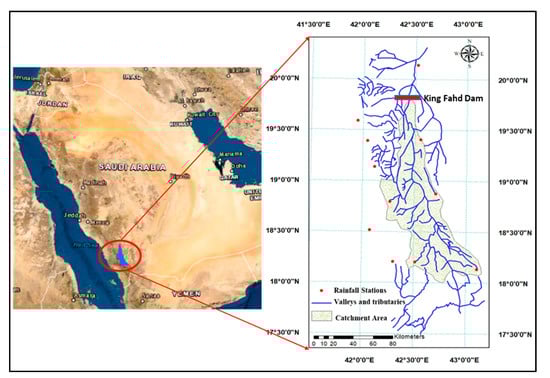
Figure 1.
Geographic location of the study area.
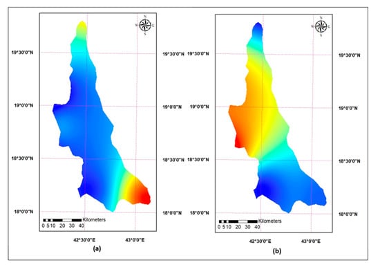
Figure 2.
(a) Average annual rainfall (1968–2019). (b) Spatial trends in the annual rainfall in the study area (1968–2019).
2.2. Hidden Markov Model (HMM)
The Markov chain is a probabilistic model that relies on probability theory and is employed to describe influences between consecutive observations of a random variable [50,51]. HMM is a limited arrangement of states that all have a typically multidimensional probability distribution linked to them and the transition between these states is controlled by transition probabilities. Outcomes or observations are produced in any of these states according to the related probability distribution. HMM comprises the context where the measurement is a probability function of the state, in which case the developed model is a doubled encoded stochastic mechanism with an implicit stochastic process that is hidden and can only be detected by another series of stochastic processes that generate the sequence of measurements [52,53]. In the Markov chain model, the outputs at time t depend explicitly on the outputs at time t-1, but the outputs in HMM are contingently independent [54]. The implementation of HMM involves the definition of two model parameters (number of states ‘N’ and the number of possible observation objects in each state ‘M’), as well as three likelihood measurements for the entire parameter range of the model, which are given by [55,56]:
where A denotes the transition probability matrix of the states, B is the emission matrix, and represents the initial distribution of the states. The following equations are used to determine these parameters:
where:
denotes the observations.
A trellis diagram of 6 HMM states that describes likelihood calculations of the implemented HMM in this study is shown in Figure 3. Each column in the diagram represents the likely state of reservoir inflow at a given time n. The transition probability represented by ai,j links each state in any specified column to each state in subsequent columns as seen in Figure 3.
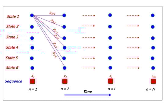
Figure 3.
Trellis diagram showing the general architecture of six hidden Markov model (HMM) states.
2.3. Support Vector Machine (SVM) Model
SVM is a classic machine learning technique focused on mathematical learning theory and it has several benefits in the classification of massive data, feature identification, and regression analysis [46]. The aim of regression analysis with SVR is to estimate a function based on the given dataset (x, y), where x represents the input vector (in this case, the input vectors (x) refer to lagged precipitation and lagged inflow) and y represents the output (referring to forecasted values). The SVM regression function can be described as follows:
in which f(x) represents the model’s output, φ(x) is representative of a nonlinear mapping function. ω and b are, respectively, the weight vector and the bias term to be optimized based on the regularized function as follows:
in which C is the penalization parameter used to balance the empirical risk and model regularization term , and represent the positive slack variable. The above SVR model is solved using Lagrange multipliers:
herein is the kernel function; and are the positive Lagrange multipliers, respectively.
Ultimately, the parameters of the SVM model are determined after reaching the desired solution for the objective function, and the regression form for an input vector x can be represented as follows:
2.4. Adaptive Neuro-Fuzzy Inference System
The ANFIS model is a fuzzy inference model (FIS) constructed as ANN, which combines the benefits of FIS with a learning algorithm [57,58]. ANFIS hypothesizes the FIS model using different output or input data, and then updates its membership criteria using a backpropagation algorithm. In the present study, ANFIS was utilized to derive the relationships between the time of year (months), lagged precipitation, lagged inflow, and the reservoir inflow and to describe them as fuzzy if–then rules as shown in Figure 2. The ANFIS model is mainly comprised of a Sugeno-type FIS of a typical bell input membership function with five functions for each input of the nine inputs, and one output with a linear membership function.
Figure 4 describes the ANFIS system with a multilayered feed-forward design that was connected to an incoherent x and y input network. The Sugeno model (Figure 5) has a rule base that takes the following form:
where fi is the output within the inconsistent zone defined by the FIS principle, Ai and Bi are the membership magnitudes, represent indirect identification function, and pi, qi, and ri are the consequential constraints adjusted in the forward passes of the learning algorithm. If the membership functions of the fuzzy sets Ai and Bj are and correspondingly, the five layers that incorporate ANFIS are described in Figure 6. More details about ANFIS can be found in Abuhasel [58].
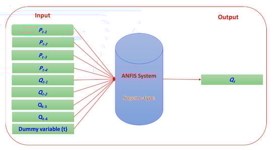
Figure 4.
An adaptive neuro-fuzzy inference system (ANFIS) architecture for inflow forecasting.
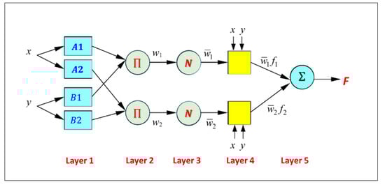
Figure 5.
Basic structure of ANFIS with a two-rule Sugeno system.
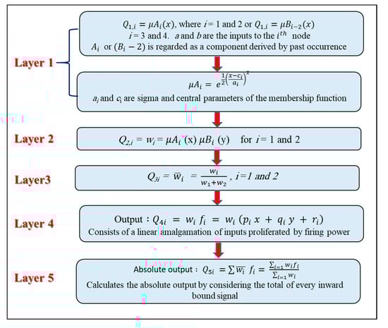
Figure 6.
Schematic diagram of the five layers that incorporate ANFIS.
2.5. Genetic Algorithm
GAs are heuristic search techniques that can be used to solve a variety of practical optimization problems. The basic concepts of GAs were initially introduced by John Holland in the 1970s, and these techniques are based on natural genetics’ evolutionary theory. A basic GA process typically consists of four steps: fitness assessment, selection, genetic operations, and substitution. A population pool of chromosomes persists in a basic GA loop. The chromosomes represent the encoded arrangement of the possible solutions, and these solutions are used for all GA operations excluding the fitness assessment. The population is originally established randomly, and the optimal solutions of all chromosomes are determined by computing the objective function in the decoded form of chromosomes. The GA evolution process starts after the population pool has been initialized. The mating pool is created at the start of each generation by selecting certain chromosomes from the population. The offspring’s fitness results are also assessed, then some chromosomes in the population will be substituted by offspring according to the substitution scheme at the end of the generation. The generation process is iterated until the termination conditions are satisfied. By simulating natural selection and genetic operations, the best chromosomes or optimal solutions can emerge in the final population.
In this study, the GA algorithm was employed to solve the single-objective optimization problem and used for updating two ANFIS parameter types: premise parameters and consequent parameters. Premise parameters correspond to the function of gauss membership described as {ai} in Figure 6. In all membership functions, the cumulative number of premise parameters is equivalent to the summation of the parameters. Consequent parameters are those used in the defuzzification layer, shown in Figure 6 as {𝑝𝑖, qi, ri}. These parameters are optimized with GA to reduce the difference between the ANFIS output and the measured data to a minimum. In SVM modeling, as the RBF was used, the GA was applied to optimize the parameters σ, C, and ε during the training process. The RMSE function obtained with Equation (17) is used to determine the error value of the solution. The RMSE represents the model’s perfect fitting to the datasets and illustrates how the observed data are closely related to the forecasted values.
2.6. Performance Evaluation of the Developed Models
To measure the performance of the ANFIS and SVM models in forecasting the reservoir inflow, the following four statistical indicators were utilized:
- Nash-Sutcliffe efficiency coefficient (NSE) [59], expressed as:
- The mean absolute error (MAD), expressed as:
- The absolute variance fraction, R2, is calculated as follows:
- The root-mean-square error (RMSE), expressed as:where Qo is the measured inflow, n is the number of data points, Qf is the forecasted inflow, and is the average of the observed reservoir inflows.
2.7. Methodology
Based on the methods discussed above, the following steps were adopted to carry out this study (Figure 7):
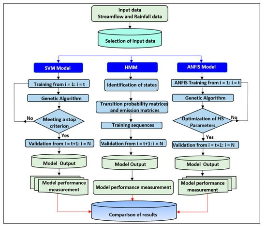
Figure 7.
Schematic diagram of the methodology presented in this study.
- ▪
- First of all, the quality of the investigated rainfall records was examined through absolute homogeneity tests to select homogeneous climate data series. These tests included Buishand range test, Von Neumann ratio test, and Standard normal homogeneity test. More details about these tests are described by Khadr [60].
- ▪
- The forecasting model was then selected and, consequently, the required input data.
- ▪
- The input data of the HMM model included the inflow; however, in SVM and ANFIS models, it included the data shown in Figure 4.
- ▪
- The input datasets were split into two sets, namely, training (70% of the data) and testing datasets (30% of the data).
- ▪
- The input variables were identified based on the selected model (HMM, SVM, and ANFIS).
- ▪
- The process of model training was then performed to obtain the best evaluation parameters.
- ▪
- The selected forecasting model was then tested, and the model performance was evaluated using the evaluation criteria (Equations (14)–(17)).
- ▪
- Finally, the historical observed inflow data are compared with the forecasted inflow from HMM, SVM, ANFIS, hybrid SVM-GA, and hybrid ANFIS-GA models.
3. Results
3.1. HMM
Inflow records were classified for the individual months (January to December), then its relative frequencies were determined, and, eventually, reservoir inflow was forecasted by HMM. Model parameters were then calculated utilizing the training dataset (39 years), and, finally, the forecasting model was validated using the remaining 16 years of data. The HMM modeling process starts with the characterization of states and how they are linked, followed by estimation of the value of parameters, and, finally, transition and emission probabilities. Table 1 represents the six considered states of inflow. The proposed approach was evaluated on various models by adjusting the parameters over appropriate domains and selecting the values that result in the least difference between forecasted and observed values. The forward-back (Baum-Welch) algorithm was employed to estimate the model, as defined in [52]. Figure 8 presents a comparison between historical and forecasted inflow values, and Table 2 demonstrates the performance measures of the proposed HMM and displays the variations in R2, RMSE, MAD, and E. For the training phase, the performance measures were R2 = 0.683, RMSE = 9.76E + 06 m3, MAD = 3.75E + 06 m3, and E = 0.643; and these measures for the testing phase were R2 = 0.370, RMSE = 1.95E + 07 m3, MAD = 1.04E + 07 m3, and E = −0.735.

Table 1.
Classification of inflow states.
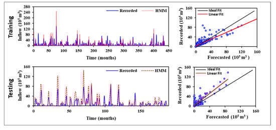
Figure 8.
Training and testing results of the simulated monthly inflow based on HMM.
Table 2.
Performance criteria of the developed models for inflow forecasting.
3.2. SVM and Hybrid SVM-GA Models
The programming of SVM was performed using MATLAB and the RBF kernel with the parameters (C, σ, ε) was employed for inflow forecasting, with the SVM model’s accuracy being dependent on the identified parameters. During the training process, the optimal selection of the SVM parameters was achieved using GA to optimize the RMSE with a population size of 100, a crossover rate of 0.8, and a mutation rate of 0.01. Once the best performing SVM model was selected through the training process, the forecast values of the selected performance were estimated, and the forecasted and measured values were compared. Figure 9 illustrates the measured and forecasted inflow and scatter plot for the SVM and SVM-GA models during the training and testing phases. The results showed that further improvements were achieved by the SVM-GA model on forecasted inflow in terms of reduced scatter. The performance criteria show that the SVM-GA model performed better than the SVM. In the case of the SVM model, for the training phase the performance measures were R2 = 0.703, RMSE = 9.19E + 06 m3, MAD = 3.71E + 06 m3, and E = 0.683; and for the testing phase were R2 = 0.581, RMSE = 1.18E + 07 m3, MAD = 6.47E + 06 m3, and E = 0.363. Considering, the performance indices, the SVM-GA model has better accuracy than the SVR model where the performance measures are R2 = 0.73, RMSE = 7.42E + 06 m3, MAD = 3.18E + 06 m3, and E = 0.794 during training; and these values for the testing period are R2 = 0.674, RMSE = 1.22E + 07 m3, MAD = 6.98E + 06 m3, and E = 0.322. A significant drop in the performance level can be observed in Figure 9 in terms of training and test results.
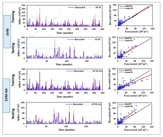
Figure 9.
Training and testing results of the simulated monthly inflow based on SVM and SVM-GA models.
3.3. ANFIS and Hybrid ANFIS-GA Models
The dataset utilized in the SVM and HMM models was employed in the ANFIS models to construct a Sugeno-type FIS using subtractive clustering. The next step involved calculating the corresponding estimate of each rule’s equation to encompass the space of the features using linear least-squares estimates. The forecasted values of the inflow were computed when the model with the best performance was identified through ANFIS training. Figure 10 shows the inflow values forecasted by ANFIS versus the observed records for both the training and testing phases. It can be clearly seen that the two curves closely converge, and the trend between the forecasted and measured data is identical, with the exception of a few records that deviate further from the historical recorded values. The high R2 value (0.857) indicates that the forecasted and measured inflow are in complete agreement. The E values in Table 2 are greater than 0.80, indicating that the developed ANFIS model has a perfect match for inflow in both testing and training phases.
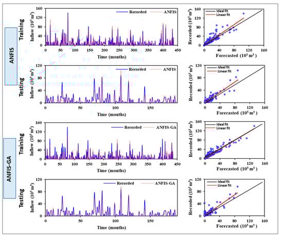
Figure 10.
Training and testing results of the simulated monthly inflow based on the ANFIS and ANFIS-GA models.
To create the ANFIS-GA model, there were twelve membership functions for each input; a total of 96 functions were composed. Two premise criteria were used in each of the membership functions. Therefore, 192 parameters were successfully optimized. During the network learning process, the optimal selection of the parameters related to the membership functions was achieved using the GA with a population size of 200, a crossover rate of 0.8, and a mutation rate of 0.01. Once the optimal performing ANFIS model was selected through ANFIS training, the forecast values of the selected performance were estimated, then the forecasted and recorded values were compared as presented in Figure 10. Table 2 indicates that the ANFIS-GA model produced accurate results compared with other models. The ANFIS model had a small drop in performance quality (R2, RMSE, and MAD) from the training to the testing phase. A much more distinctive description arises in Figure 6, which illustrates the disparity between the forecasted and measured inflow in the training and testing phases, as well as comparative scatter plots. According to the time series plots, the ANFIS-GA model was proficient at recognizing the fluctuating pattern of the measured inflow and there was a higher consensus in the forecasted peak values in comparison to their measured records.
4. Discussion and Comparison of the Developed Forecasting Models
This study compared the hydrological performance of five forecasting models in reservoir inflow forecasting, i.e., HMM, SVM, SVM-GA, ANFIS, and ANFIS-GA. The comprehensive analysis performed in the evaluation of the five models (Table 2) identified variety in the performance of these models. The statistical indices utilized to evaluate the developed models (R2, RMSE, MAD, and E) revealed that the ANFIS-GA model outperformed the other four forecasting models, and it produced the highest R2, the minimum RMSE, and maximum value of E. The ANFIS and SVM model showed a slight decrease in the level of performance from the training phase to the testing phase; however, the drop in performance measures obtained by HMM was relatively high. Based on the statistical indices in Table 2, it can be determined that the models combined with GA performed much better than the stand-alone SVM and ANFIS models and GA improves the accuracy of forecasting in both training and testing periods. Consequently, the RMSE values of SVM-GA model have been reduced by 19.26 and 3.38% in comparison with the results of the SVM model at training and test processes, respectively. The RMSE values of ANFIS-GA model have been reduced by 30.40 and 8.48% in comparison with the results of the ANFIS model at training and test processes, respectively. In addition, the R2 values of SVM model have been increased by 4.28 and 11.35% in comparison with the results of the SVM model at training and test processes, respectively. However, the R2 values of ANFIS-GA model have been increased by 8.85 and 4.5% in comparison with the results of the ANFIS model at training and testing processes, respectively. These results indicate the GA-induced improvement in both the SVM and ANFIS model due to the capability of GA in finding the parameters of the optimal solution of SVM and ANFIS models.
To further investigate the models’ performance, an additional statistical evaluation was also carried out using the Taylor diagram, which describes the statistical characteristics of the developed models and their relative positions from the observed dataset during the training and testing phases (Figure 11) based on RMSE and the triangle inequality comparison. Figure 11 illustrates that the ANFIS-GA model performed better than the other model as it was the closest model to the reference line (RMSE) and observed datasets. Few hydrological studies have used hybrid ANFIS and SVM models to predict reservoir monthly inflow.
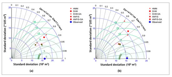
Figure 11.
Taylor diagram for HMM, SVM, SVM-GA, ANFIS, and ANFIS-GA compared to the observed data. (a) Training (b) Testing.
The finding of our study supported and agrees with the results previous studies [61,62,63,64], which reported that employing hybrid model enhance the forecasting accuracy of the stand-alone model. For instance, Yaseen et al. [61] used firefly algorithm as an optimizer tool to construct a hybrid ANFIS-FFA mode for inflow forecasting. The comparison of their results revealed that the FFA was able to improve the forecasting accuracy of the hybrid, as R2 increased by 0.40% and RMSE decreased by 69.5%. Shafaei and Kisi [62] reported that using of wavelet-ANN in predicting daily river flow increased R2 by 7.38% and 7.40%, and decreased MSE by 56.14% and 55% in comparison with the results of the stand-alone ANN model at training and test processes, respectively. Furthermore, their results revealed that the proposed hybrid ANN model outperforms the ANN and SVM models, according to the comparison data. Zhou et al. [63] proposed a recurrent ANFIS model for multistep-ahead forecasting using a genetic algorithm and least square estimator for parameters optimization. Their results illustrated that the proposed model has the potential to have much more reliable forecasting of the inflow sequence of over a long forecast period compared with the stand-alone ANFIS model as the RMSE values have been decreased by 14.80 and 14.08% at training and test processes, respectively. Su et al. [64] found that the employing GA to optimize the parameters of the SVM improved the accuracy of the monthly inflow forecasting compared with other optimization algorism such as grid search and particle swarm optimization methods. Their results revealed that utilizing GA instead of grid search to optimize the SVM’s parameters increased R2 by 2.04% and de-creased RMSE by 78.9% at test process. Furthermore, our work provides new insights into the use of hybrid ANFIS to forecast reservoir monthly inflow.
5. Conclusions
In this study, we examined the potential of the HMM, SVM-GA, and ANFIS-GA models for the one-month-ahead forecasting of reservoir inflow. The constructed models were then evaluated by the historical monthly data of the King Fahd dam, Saudi Arabia. Four statistical measures were utilized to evaluate the performance of the established models and a Taylor diagram was presented to assess the correspondence between the historical inflow output and that of each model. Generally, the results showed that ANFIS and SVM models provided more accurate forecasting than HMM as a statistical model. In terms of the performance outcomes of the developed models, the comparison of the results demonstrated that the ANFIS model is more capable of capturing monthly inflows than the SVM and HMM models. Indeed, employing GA as an add-in optimization algorithm in the ANFIS and SVM models improved the forecasting performance of both models significantly. Based on the results and discussion, the main conclusion of this study is that integrating ANFIS and SVM with GA would result in a highly valuable tool for monthly inflow forecasting in the study area.
Author Contributions
Conceptualization, M.M.A., K.A.A., and M.K.; Data curation, M.M.A., K.A.A., and M.K.; Formal analysis, M.M.A., K.A.A., A.S.A., and M.K.; Funding acquisition, M.M.A.; Methodology, M.M.A., K.A.A., A.S.A., and M.K.; Project administration, M.M.A.; Resources, M.M.A.; Software, M.M.A., K.A.A., A.S.A., and M.K.; Supervision, M.M.A.; Validation, A.S.A. and M.K.; Visualization, K.A.A., and A.S.A.; Writing—original draft, A.S.A. and M.K.; Writing—review and editing, K.A.A. and M.K. All authors have read and agreed to the published version of the manuscript.
Funding
This research was funded by Deputyship for Research & Innovation, Ministry of Education in Saudi Arabia, grant number 17.
Institutional Review Board Statement
Not applicable.
Informed Consent Statement
Not applicable.
Data Availability Statement
The data that support the findings of this study are available from the Ministry of Environment Water and Agriculture, Saudi Arabia, but restrictions apply to the availability of these data, which were used for the current study, and so are not publicly available.
Acknowledgments
The authors extend their appreciation to the Deputyship for Research & Innovation, Ministry of Education in Saudi Arabia, for funding this research work through project number 17.
Conflicts of Interest
The authors declare no conflict of interest. The funders had no role in the design of the study, in the collection, analyses, or interpretation of data, in the writing of the manuscript, or in the decision to publish the results.
References
- Apaydin, H.; Feizi, H.; Sattari, T.M.; Colak, S.M.; Shamshirband, S.; Chao, W.K. Comparative analysis of recurrent neural network architectures for reservoir inflow forecasting. Water 2020, 12, 1500. [Google Scholar] [CrossRef]
- Peng, T.; Zhou, J.; Zhang, C.; Fu, W. Streamflow forecasting using empirical wavelet transform and artificial neural networks. Water 2017, 9, 406. [Google Scholar] [CrossRef]
- Kompor, W.; Yoshikawa, S.; Kanae, S. Use of Seasonal Streamflow Forecasts for Flood Mitigation with Adaptive Reservoir Operation: A Case Study of the Chao Phraya River Basin, Thailand, in 2011. Water 2020, 12, 3210. [Google Scholar] [CrossRef]
- Lee, S.-Y.; Hamlet, A.F.; Fitzgerald, C.J.; Burges, S.J. Optimized flood control in the Columbia River Basin for a global warming scenario. J. Water Resour. Plan. Manag. 2009, 135, 440–450. [Google Scholar] [CrossRef]
- Chang, J.; Meng, X.; Wamg, Z.Z.; Wamg, X.; Huang, Q. Optimized cascade reservoir operation considering ice flood control and power generation. J. Hydrol. 2014, 519, 1042–1051. [Google Scholar] [CrossRef]
- Hsu, N.-S.; Huang, C.-L.; Wei, C.-C. Multi-phase intelligent decision model for reservoir real-time flood control during typhoons. J. Hydrol. 2015, 522, 11–34. [Google Scholar] [CrossRef]
- Raso, L.; Chiavico, M.; Dorchies, D. Optimal and centralized reservoir management for drought and flood protection on the Upper Seine–Aube river system using stochastic dual dynamic programming. J. Water Resour. Plan. Manag. 2019, 145, 05019002. [Google Scholar] [CrossRef]
- Shen, X. Flood Risk Perception and Communication within Risk Management in Different Cultural Contexts. A Comparative Case Study between Wuhan, China, and Cologne, Germany; UNU-EHS: Bonn, Germany, 2010. [Google Scholar]
- Chan, N.W. Impacts of Disasters and Disaster Risk Management in Malaysia: The Ccase of Floods, in Resilience and Recovery in Asian Disasters; Springer: Berlin/Heidelberg, Germany, 2015; pp. 239–265. [Google Scholar]
- Zhong, Y.; Guo, S.; Ba, H.; Xiong, F.; Chang, F.J.; Lin, K. Evaluation of the BMA probabilistic inflow forecasts using TIGGE numeric precipitation predictions based on artificial neural network. Hydrol. Res. 2018, 49, 1417–1433. [Google Scholar] [CrossRef]
- Ding, Z. Overview of Measures and Assessment of Capacity for Flood Prevention and Drought Relief, in Flood Prevention and Drought Relief in Mekong River Basin; Springer: Berlin/Heidelberg, Germany, 2020; pp. 109–166. [Google Scholar] [CrossRef]
- Di Baldassarre, G.; Martinez, F.; Kalantari, Z.; Viglione, A. Drought and flood in the Anthropocene: Feedback mechanisms in reservoir operation. Earth Syst. Dyn. 2017, 8, 1–9. [Google Scholar] [CrossRef]
- Shrestha, B.B.; Kawasaki, A. Quantitative assessment of flood risk with evaluation of the effectiveness of dam operation for flood control: A case of the Bago River Basin of Myanmar. Int. J. Disaster Risk Reduct. 2020, 50, 101707. [Google Scholar] [CrossRef]
- Bai, Y.; Sun, Z.; Zeng, B.; Long, J. Reservoir inflow forecast using a clustered random deep fusion approach in the Three Gorges Reservoir, China. J. Hydrol. Eng. 2018, 23, 04018041. [Google Scholar] [CrossRef]
- Amnatsan, S.; Yoshikawa, S.; Kanae, S. Improved forecasting of extreme monthly reservoir inflow using an analogue-based forecasting method: A case study of the sirikit dam in Thailand. Water 2018, 10, 1614. [Google Scholar] [CrossRef]
- Coulibaly, P.; Haché, M.; Fortin, V.; Bobée, B. Improving daily reservoir inflow forecasts with model combination. J. Hydrol. Eng. 2005, 10, 91–99. [Google Scholar] [CrossRef]
- Zhang, Z.; Zhang, Q.; Singh, V.P. Univariate streamflow forecasting using commonly used data-driven models: Literature review and case study. Hydrol. Sci. J. 2018, 63, 1091–1111. [Google Scholar] [CrossRef]
- Wang, Z.-Y.; Qiu, J.; Li, F.-F. Hybrid models combining EMD/EEMD and ARIMA for Long-term streamflow forecasting. Water 2018, 10, 853. [Google Scholar] [CrossRef]
- Zhou, J.; Peng, T.; Zhang, C.; Sun, N. Data pre-analysis and ensemble of various artificial neural networks for monthly streamflow forecasting. Water 2018, 10, 628. [Google Scholar] [CrossRef]
- Valipour, M. Long-term runoff study using SARIMA and ARIMA models in the United States. Meteorol. Appl. 2015, 22, 592–598. [Google Scholar] [CrossRef]
- Moeeni, H.; Bonakdari, H.; Ebteha, I. Integrated SARIMA with neuro-fuzzy systems and neural networks for monthly inflow prediction. Water Resour. Manag. 2017, 31, 2141–2156. [Google Scholar] [CrossRef]
- Moeeni, H.; Bonakdari, H.; Ebteha, I. Monthly reservoir inflow forecasting using a new hybrid SARIMA genetic programming approach. J. Earth Syst. Sci. 2017, 126, 18. [Google Scholar] [CrossRef]
- Moeeni, H.; Bonakdari, H.; Fatemi, S.H.; Zaji, A.H. Assessment of stochastic models and a hybrid artificial neural network-genetic algorithm method in forecasting monthly reservoir inflow. INAE Lett. 2017, 2, 13–23. [Google Scholar] [CrossRef][Green Version]
- Chaiwattana, P.; Suiadee, W.; Songchon, C. Forecasting for hydrological data for reservoir sizing: Case study huai tha koei reservoir. In Proceedings of the 2ndworld Irrig Forum (Wif2), Chiang Mai, Thailand, 6–8 November 2016. [Google Scholar]
- Ehteram, M.; Afan, H.A.; Dianatickhah, M.; Ahmed, A.J.; Fai, C.M.; Hossain, M.S.; Allawi, M.F.; Elshafie, A. Assessing the predictability of an improved ANFIS model for monthly streamflow using lagged climate indices as predictors. Water 2019, 11, 1130. [Google Scholar] [CrossRef]
- Chang, L.-C.; Amin, M.Z.M.; Yang, S.N.; Chang, F.J. Building ANN-based regional multi-step-ahead flood inundation forecast models. Water 2018, 10, 1283. [Google Scholar] [CrossRef]
- Kişi, Ö. River flow modeling using artificial neural networks. J. Hydrol. Eng. 2004, 9, 60–63. [Google Scholar] [CrossRef]
- Khadr, M.; Schlenkhoff, A. Data-driven stochastic modeling for multi-purpose reservoir simulation. J. Appl. Water Eng. Res. 2018, 1, 40–47. [Google Scholar] [CrossRef]
- Noori, R.; Karbassi, A.R.; Mehdizadeh, H.; Vesali, N.M.; Sabahi, M.S. A framework development for predicting the longitudinal dispersion coefficient in natural streams using an artificial neural network. Environ. Prog. Sustain. Energy 2011, 30, 439–449. [Google Scholar] [CrossRef]
- Kişi, Ö. Neural networks and wavelet conjunction model for intermittent streamflow forecasting. J. Hydrol. Eng. 2009, 14, 773–782. [Google Scholar] [CrossRef]
- Adnan, R.M.; Yuan, X.; Kisi, O.; Yuan, Y. Streamflow forecasting using artificial neural network and support vector machine models. Am. Sci. Res. J. Eng. Technol. Sci. 2017, 29, 286–294. [Google Scholar]
- Dariane, A.B.; Azimi, S. Streamflow forecasting by combining neural networks and fuzzy models using advanced methods of input variable selection. J. Hydroinform. 2018, 20, 520–532. [Google Scholar] [CrossRef]
- Mohammadi, K.; Eslami, H.; Dayani, D.S. Comparison of regression, ARIMA and ANN models for reservoir inflow forecasting using snowmelt equivalent (a case study of Karaj). J. Agric. Sci. Technol. 2005, 7, 17–30. [Google Scholar]
- Valipour, M.; Banihabib, M.E.; Behbahani, S.M.R. Comparison of the ARMA, ARIMA, and the autoregressive artificial neural network models in forecasting the monthly inflow of Dez dam reservoir. J. Hydrol. 2013, 476, 433–441. [Google Scholar] [CrossRef]
- Zhang, G.P. Time series forecasting using a hybrid ARIMA and neural network model. Neurocomputing 2003, 50, 159–175. [Google Scholar] [CrossRef]
- Cheng, C.-T.; Feng, Z.K.; Niu, W.J.; Liao, S.L. Heuristic methods for reservoir monthly inflow forecasting: A case study of Xinfengjiang Reservoir in Pearl River, China. Water 2015, 7, 4477–4495. [Google Scholar] [CrossRef]
- Mosavi, A.; Ozturk, P.; Chau, K.-W. Flood prediction using machine learning models: Literature review. Water 2018, 10, 1536. [Google Scholar] [CrossRef]
- Dibike, Y.B.; Velickov, S.; Solomatine, D.; Abott, M.B. Model induction with support vector machines: Introduction and applications. J. Comput. Civ. Eng. 2001, 15, 208–216. [Google Scholar] [CrossRef]
- Parsaie, A.; Yonesi, H.A.; Najafian, S. Predictive modeling of discharge in compound open channel by support vector machine technique. Modelling Earth Syst. Environ. 2015, 1, 1. [Google Scholar] [CrossRef]
- Kisi, O. Streamflow forecasting and estimation using least square support vector regression and adaptive neuro-fuzzy embedded fuzzy c-means clustering. Water Resour. Manag. 2015, 29, 5109–5127. [Google Scholar] [CrossRef]
- Ghorbani, M.A.; Khatibi, R.; Goel, A.; Falezi, F.H.A.; Azani, A. Modeling river discharge time series using support vector machine and artificial neural networks. Environ. Earth Sci. 2016, 75, 685. [Google Scholar] [CrossRef]
- Chau, K.; Wu, C.; Li, Y. Comparison of several flood forecasting models in Yangtze River. J. Hydrol. Eng. 2005, 10, 485–491. [Google Scholar] [CrossRef]
- Long, Y.; Tang, R.; Wang, H.; Jiang, C. Monthly precipitation modeling using Bayesian non-homogeneous hidden Markov chain. Hydrol. Res. 2019, 50, 562–576. [Google Scholar] [CrossRef]
- Khadr, M. Forecasting of meteorological drought using Hidden Markov Model (case study: The upper Blue Nile river basin, Ethiopia). Ain Shams Eng. J. 2016, 7, 47–56. [Google Scholar] [CrossRef]
- Hernández, L.C.H.; Reis, D.S., Jr. Seasonal Inflow Forecasts Based on Non-Homogeneous Hidden Markov Models: The Case of Orós Reservoir, Northeastern Brazil. In World Environmental and Water Resources Congress 2018: Watershed Management, Irrigation and Drainage, and Water Resources Planning and Management; American Society of Civil Engineers: Reston, VA, USA, 2018; pp. 269–277. [Google Scholar]
- Rolim, L.Z.R.; de Souza Filho, F.D.A. Shift Detection in Hydrological Regimes and Pluriannual Low-Frequency Streamflow Forecasting Using the Hidden Markov Model. Water 2020, 12, 2058. [Google Scholar] [CrossRef]
- Hernadez, H.L.C.; Silveira, R.D., Jr. Forecasting inflow persistence using climate-informed Hidden Markov Models: An Application to Orós Reservoir in Brazil. In Proceedings of the 20th EGU General Assembly, EGU2018. Vienna, Austria, 4–13 April 2018; p. 16889. [Google Scholar]
- Keilson, J. Markov chain models--rarity and exponentiality. In Applied Mathematical Ssciences; Springer: New York, NY, USA, 1979; p. 184. [Google Scholar]
- Liu, Y.; Ye, L.; Qin, H.; Hong, X.; Ye, J.; Yin, X. Monthly streamflow forecasting based on hidden Markov model and Gaussian Mixture Regression. J. Hydrol. 2018, 561, 146–159. [Google Scholar] [CrossRef]
- Elliott, R.J.; Aggoun, L.; Moore, J.B. Hidden Markov Models: Estimation and Control. In Applications of Mathematics; Springer: New York, NY, USA, 1995; p. 361. [Google Scholar]
- MacDonald, I.L.; Zucchini, W. Hidden Markov and other models for discrete-valued time series. In Monographs on Statistics and Applied Probability, 1st ed.; Chapman & Hall: New York, NY, USA; London, UK, 1997; p. 236. [Google Scholar]
- Zucchini, W.; MacDonald, I.L. Hidden Markov models for time series: An introduction using R. In Monographs on Statistics and Applied Probability; CRC Press: Boca Raton, FL, USA, 2009; p. 275. [Google Scholar]
- Mares, I.C.M. A hidden Markov model for the Orsova discharge level in springtime. In Proceedings of the BALWOIS 2008, Ohrid, North Macedonia, 27–31 May 2008. [Google Scholar]
- Buhlmann, P.; Wyner, A.J. Variable length Markov chains. Ann. Stat. 1999, 27, 480–513. [Google Scholar] [CrossRef]
- Steeb, W.H. The Nonlinear Wrkbook : Chaos, Fractals, Cellular Automata, Neural Networks, Genetic Algorithms, Gene Expression Programming, Support Vector Machine, Wavelets, Hidden Markov Models, Fuzzy Logic with C++, Java and SymbolicC++ Programs, 4th ed.; World Scientific: New Jersey, NJ, USA, 2008; p. 605. [Google Scholar]
- Müller, K.-R.; Smol, A.J.; Rätsch, G.; Schölkopf, B.; Kohlmorgen, J.; Vapnik, V. Predicting Time Series with Support Vector Machines. In International Conference on Artificial Neural Networks; Springer: Berlin/Heidelberg, Germany, 1997. [Google Scholar]
- Zadeh, L.A. Outline of a new approach to the analysis of complex systems and decision processes. IEEE Trans. Syst. Man Cybern. 1973, 1, 28–44. [Google Scholar] [CrossRef]
- Abuhasel, K.A. Machine learning approach to handle data-driven model for simulation and forecasting of the cone crusher output in the stone crushing plant. Comput. Intell. 2020. [Google Scholar] [CrossRef]
- Nash, J.E.; Sutcliffe, J.V. River flow forecasting through conceptual models part I—A discussion of principles. J. Hydrol. 1970, 10, 282–290. [Google Scholar] [CrossRef]
- Khadr, M. Temporal and spatial patterns of rainfall variability using nonparametric methods and wavelet transform: A case study of Sinai Peninsula. Arab. J. Geosci. 2021, 14, 1–22. [Google Scholar] [CrossRef]
- Yaseen, Z.M.; Ebtehaj, I.; Bonakdari, H.; Deo, C.R.; Mehr, A.D.; Mohar, W.M.H.W.; Diop, L.; El-Shafie, A.; Singh, V.P. Novel approach for streamflow forecasting using a hybrid ANFIS-FFA model. J. Hydrol. 2017, 554, 263–276. [Google Scholar] [CrossRef]
- Shafaei, M.; Kisi, O. Predicting river daily flow using wavelet-artificial neural networks based on regression analyses in comparison with artificial neural networks and support vector machine models. Neural Comput. Appl. 2017, 28, 15–28. [Google Scholar] [CrossRef]
- Zhou, Y.; Guo, S.; Chang, F.J. Explore an evolutionary recurrent ANFIS for modelling multi-step-ahead flood forecasts. J. Hydrol. 2019, 570, 343–355. [Google Scholar] [CrossRef]
- Su, J.; Wang, X.; Liang, Y.; Chen, B. GA-based support vector machine model for the prediction of monthly reservoir storage. J. Hydrol. Eng. 2014, 19, 1430–1437. [Google Scholar] [CrossRef]


Publisher’s Note: MDPI stays neutral with regard to jurisdictional claims in published maps and institutional affiliations. |
© 2021 by the authors. Licensee MDPI, Basel, Switzerland. This article is an open access article distributed under the terms and conditions of the Creative Commons Attribution (CC BY) license (https://creativecommons.org/licenses/by/4.0/).