
Multi-Spatial Resolution Rainfall-Runoff Modelling—A Case Study of Sabari River Basin, India


Abstract
1. Introduction
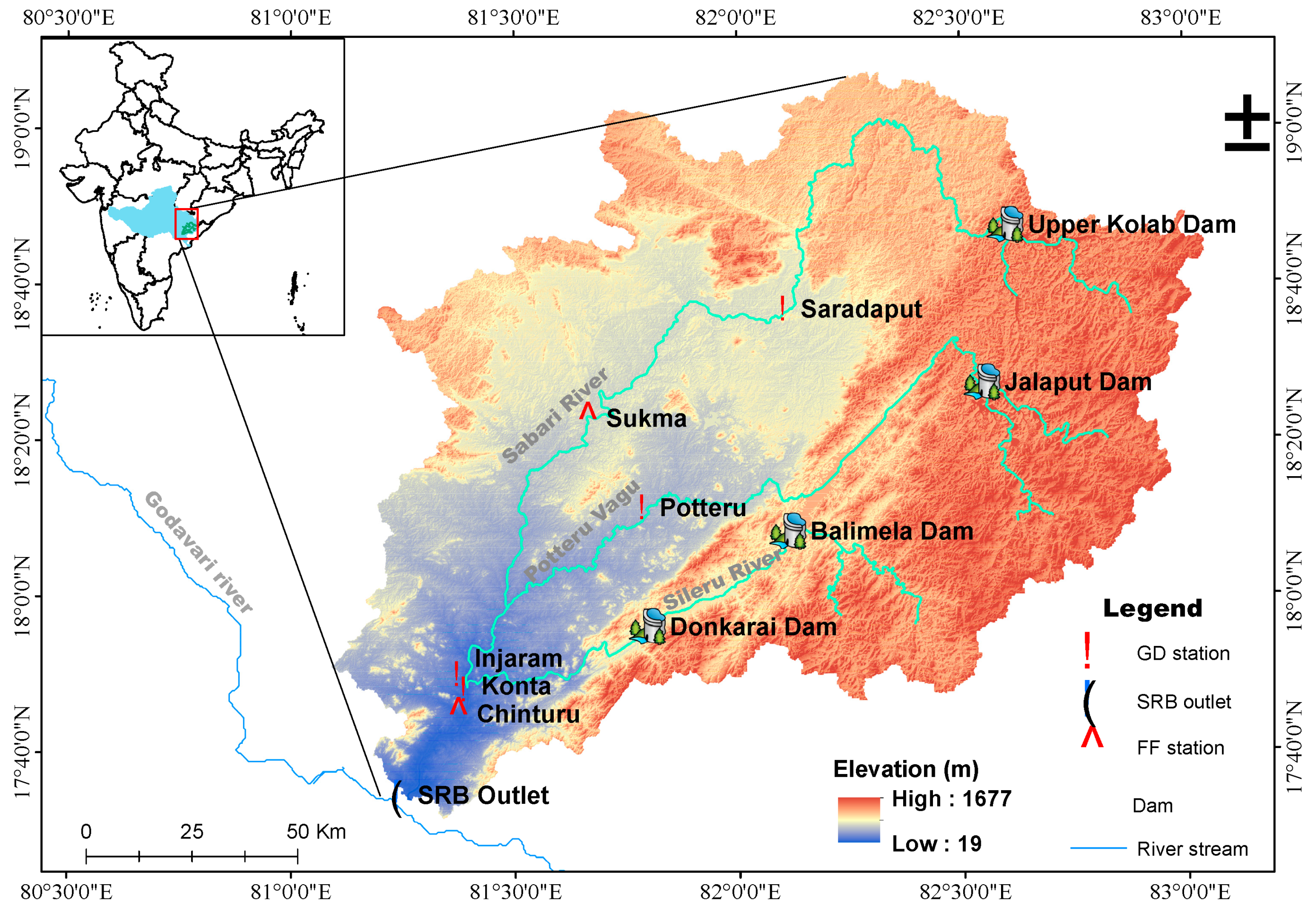
2. Study Area
3. Data
4. Methodology
4.1. Selection of Flood Events
4.2. Model Setup
4.3. Model Calibration
4.3.1. Model Initial Parameter Estimation
4.3.2. Model Parameter Optimization

| Metric | Equation | Range |
|---|---|---|
| Peak-Weighted Root Mean Square Error (PWRMSE) (m3/s) | 0 to ∞ | |
| Correlation coefficient, r | −1 to 1 | |
| Nash-Sutcliffe Efficiency, NSE | −∞ to1 | |
| Root Mean Squared Error, RMSE (m3/s) | 0 to ∞ | |
| Mean Absolute Error, MAE (m3/s) | 0 to ∞ | |
| Percent bias, PBIAS (%) | −∞ to ∞ | |
| Percentage Error in Peak, PEP (%) | −∞ to ∞ | |
| Error in Time to Peak, ETP (number of days) | −∞ to ∞ |
4.4. Model Validation
5. Results and Discussions
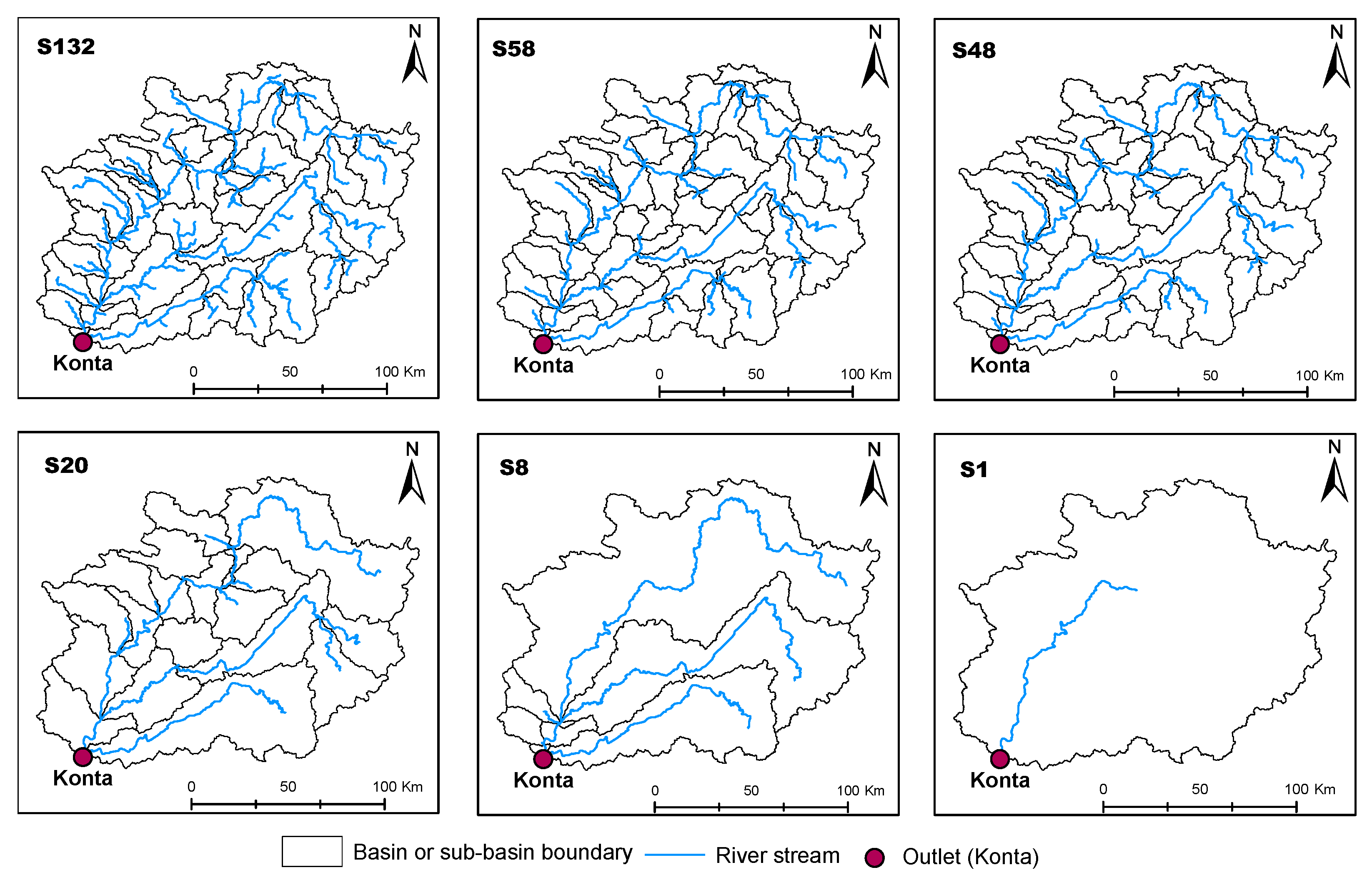
5.1. The Six Configurations of Sabari River Basin
5.2. Results from the Model Calibration
5.2.1. Spatial Resolution
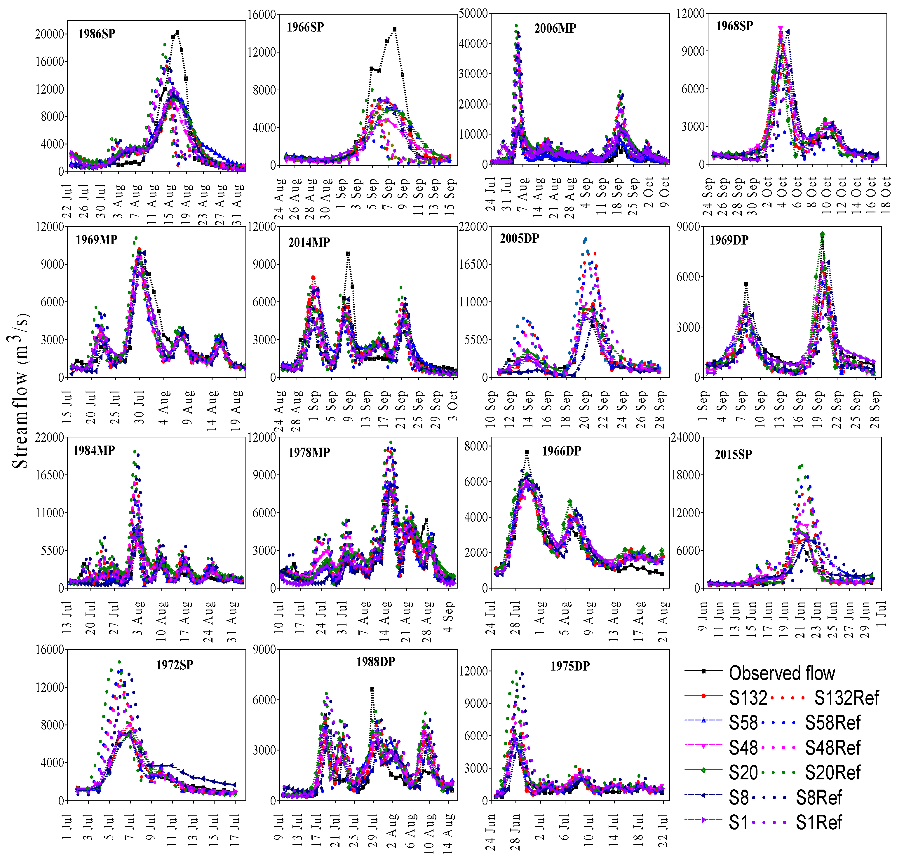
5.2.2. Selected Flood Events
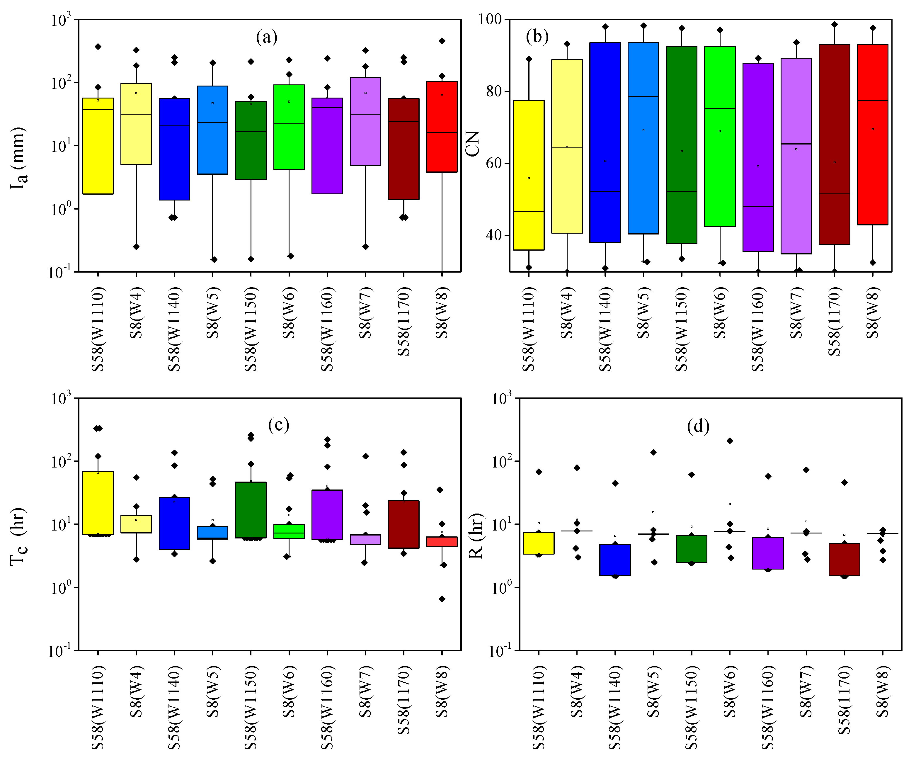
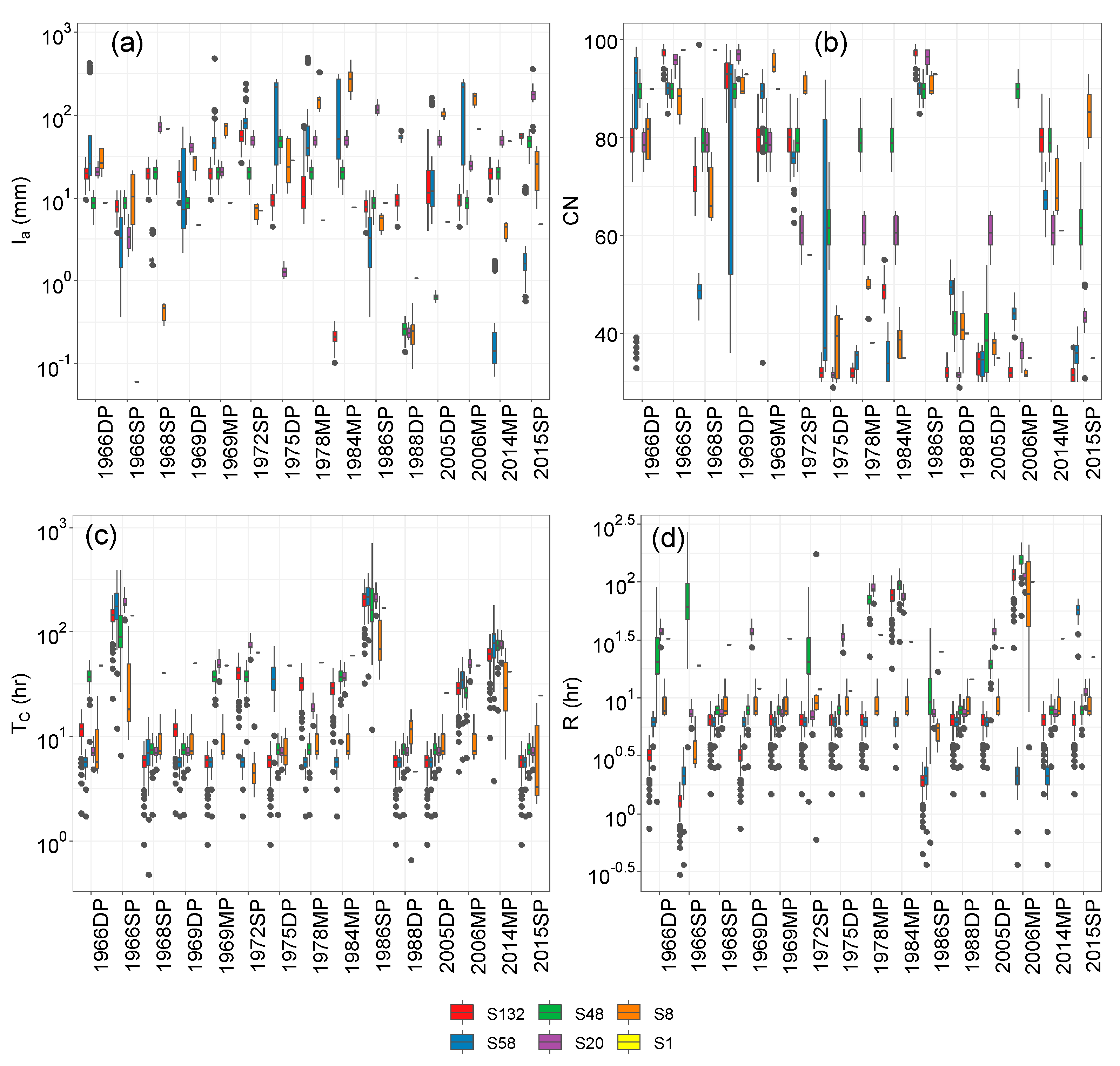
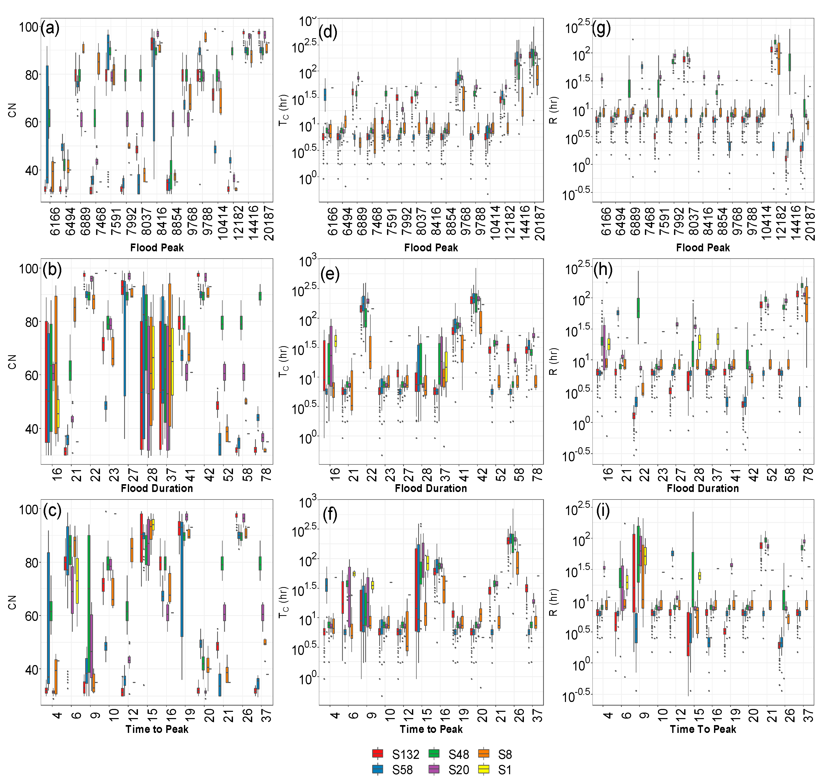
5.2.3. Event Characteristics
5.2.4. Performance Metrics
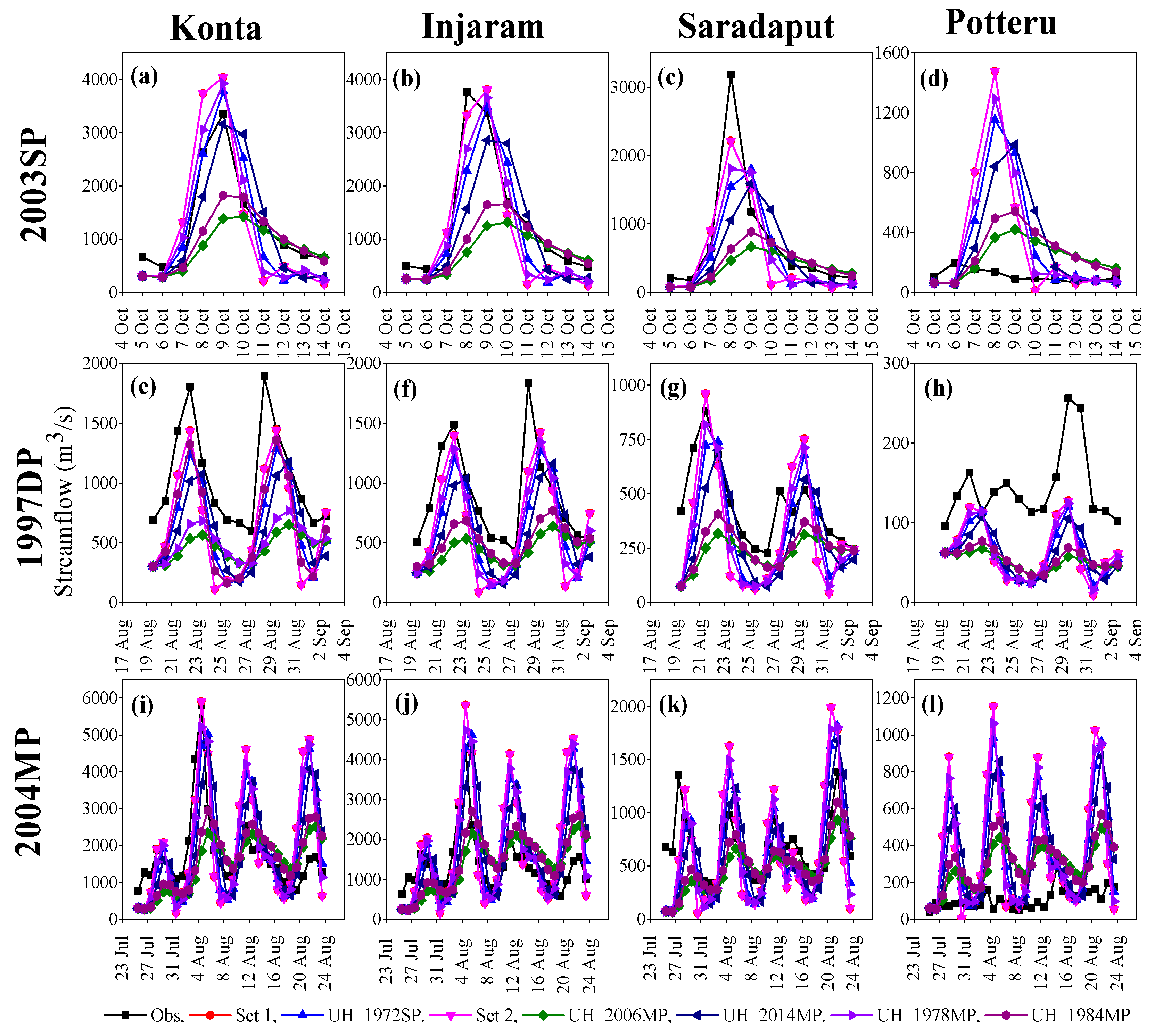
5.3. Results from the Model Validation
6. Conclusions
Supplementary Materials
Author Contributions
Funding
Institutional Review Board Statement
Informed Consent Statement
Data Availability Statement
Acknowledgments
Conflicts of Interest
Appendix A
| Event | Pearson Correlation Coefficient (r) | Nash-Sutcliffe Efficiencey (NSE) | Root Mean Square Error (RMSE) | |||||||||||||||
|---|---|---|---|---|---|---|---|---|---|---|---|---|---|---|---|---|---|---|
| S132 | S58 | S48 | S20 | S8 | S1 | S132 | S58 | S48 | S20 | S8 | S1 | S132 | S58 | S48 | S20 | S8 | S1 | |
| 1986SP | 0.47 | 0.48 | 0.52 | 0.41 | 0.58 | 0.63 | 0.15 | 0.17 | 0.23 | 0.04 | 0.31 | 0.37 | 5118.88 | 5080.12 | 4879.84 | 5455.93 | 4618.44 | 4411.23 |
| 1966SP | 0.43 | 0.40 | 0.52 | 0.32 | 0.64 | 0.71 | −0.07 | −0.28 | −0.04 | −0.11 | 0.09 | −0.01 | 4657.01 | 5111.15 | 4595.99 | 4764.48 | 4298.19 | 4534.46 |
| 1968SP | 0.93 | 0.86 | 0.96 | 0.84 | 0.85 | 0.95 | 0.82 | 0.10 | 0.86 | 0.69 | 0.67 | 0.68 | 1068.81 | 2374.82 | 924.15 | 1395.14 | 1443.25 | 1419.53 |
| 2015SP | 0.91 | 0.86 | 0.86 | 0.92 | 0.35 | 0.83 | −1.05 | −2.27 | −0.79 | −2.58 | −0.42 | −1.37 | 3019.58 | 3814.38 | 2822.60 | 3991.26 | 2518.43 | 3248.37 |
| 1972SP | 0.92 | 0.93 | 0.96 | 0.74 | 0.97 | 0.98 | −0.17 | −0.66 | 0.11 | −1.90 | −0.20 | 0.54 | 2133.86 | 2539.65 | 1859.45 | 3355.05 | 2157.22 | 1336.20 |
| 2005DP | 0.96 | 0.95 | 0.96 | 0.87 | 0.65 | 0.86 | −2.03 | −1.44 | −1.15 | −2.50 | 0.05 | −0.51 | 3836.96 | 3442.04 | 3233.00 | 4122.93 | 2147.18 | 2712.62 |
| 1969DP | 0.84 | 0.86 | 0.85 | 0.77 | 0.75 | 0.85 | 0.59 | 0.65 | 0.59 | 0.55 | 0.43 | 0.55 | 1100.69 | 1016.35 | 1092.58 | 1153.14 | 1291.11 | 1148.58 |
| 1966DP | 0.91 | 0.91 | 0.92 | 0.88 | 0.91 | 0.94 | 0.81 | 0.81 | 0.82 | 0.68 | 0.77 | 0.84 | 734.79 | 735.25 | 717.34 | 944.85 | 810.78 | 680.04 |
| 1988DP | 0.70 | 0.43 | 0.66 | 0.76 | 0.48 | 0.67 | −0.03 | 0.14 | 0.03 | −0.33 | −0.71 | −0.69 | 1322.45 | 1204.08 | 1283.42 | 1500.39 | 1698.36 | 1689.17 |
| 1975DP | 0.91 | 0.89 | 0.90 | 0.80 | 0.84 | 0.89 | −0.51 | 0.67 | 0.06 | −2.73 | −2.43 | −1.08 | 1407.16 | 659.26 | 1112.53 | 2213.73 | 2124.83 | 1655.59 |
| 2006MP | 0.63 | 0.63 | 0.67 | 0.51 | 0.74 | 0.79 | −5.44 | −4.92 | −4.38 | −6.71 | −5.38 | −2.55 | 6882.41 | 6599.83 | 6290.87 | 7531.05 | 6850.24 | 5113.00 |
| 1969MP | 0.84 | 0.84 | 0.86 | 0.75 | 0.89 | 0.94 | 0.70 | 0.71 | 0.74 | 0.48 | 0.78 | 0.85 | 1326.04 | 1315.39 | 1241.21 | 1753.40 | 1124.58 | 928.52 |
| 2014MP | 0.61 | 0.54 | 0.62 | 0.47 | 0.67 | 0.68 | 0.24 | 0.17 | 0.31 | −0.12 | 0.38 | 0.42 | 1693.96 | 1774.77 | 1614.52 | 2054.33 | 1530.16 | 1485.55 |
| 1984MP | 0.80 | 0.81 | 0.83 | 0.60 | 0.89 | 0.90 | −1.12 | −0.14 | −0.99 | −2.87 | −1.67 | −0.19 | 2332.54 | 1706.15 | 2256.04 | 3147.65 | 2614.85 | 1750.01 |
| 1978MP | 0.82 | 0.82 | 0.82 | 0.76 | 0.75 | 0.81 | −0.02 | −0.19 | 0.09 | −0.61 | −0.28 | 0.24 | 1650.69 | 1777.40 | 1557.29 | 2069.51 | 1842.01 | 1425.39 |
| Event | Mean Absolute Error (MAE) | Percent Bias (PBIAS) | Percent Error in Peak flows (PEP) | |||||||||||||||
| S132 | S58 | S48 | S20 | S8 | S1 | S132 | S58 | S48 | S20 | S8 | S1 | S132 | S58 | S48 | S20 | S8 | S1 | |
| 1986SP | 2600.49 | 2641.39 | 2528.20 | 2997.37 | 2386.76 | 2200.10 | 21.70 | 18.30 | 21.70 | 12.80 | 17.80 | 25.00 | 20.81 | 21.88 | 26.09 | 7.79 | 15.21 | 25.98 |
| 1966SP | 2446.43 | 2792.20 | 2420.88 | 2461.57 | 2271.55 | 2478.39 | 180.10 | 414.20 | 208.40 | 141.90 | 183.20 | 246.10 | 54.87 | 81.60 | 60.68 | 43.86 | 52.58 | 72.32 |
| 1968SP | 676.42 | 1372.62 | 641.37 | 864.60 | 742.86 | 699.81 | 19.10 | 162.50 | 17.80 | 16.30 | 33.00 | 43.40 | 23.45 | 72.92 | 24.04 | 14.74 | 21.70 | 50.19 |
| 2015SP | 1770.01 | 2189.63 | 1699.86 | 2353.43 | 1715.73 | 2197.38 | −52.00 | −57.10 | −50.10 | −59.20 | −27.40 | −57.40 | −99.99 | −139.32 | −93.64 | −171.65 | 1.12 | −89.48 |
| 1972SP | 1203.88 | 1391.14 | 1042.55 | 1771.96 | 1071.33 | 935.79 | −27.00 | −33.90 | −26.00 | −35.90 | −27.80 | −26.10 | −90.26 | −107.95 | −77.63 | −113.78 | −98.97 | −41.52 |
| 2005DP | 2441.92 | 2304.82 | 2245.28 | 2604.28 | 1506.53 | 1925.68 | −47.30 | −46.40 | −45.70 | −48.70 | 18.40 | −42.40 | −112.19 | −94.80 | −81.97 | −135.32 | −14.57 | −54.44 |
| 1969DP | 792.44 | 706.01 | 721.17 | 873.49 | 770.29 | 614.95 | 45.60 | 38.40 | 44.40 | 22.10 | 52.50 | 46.20 | 39.12 | 39.77 | 42.59 | 14.77 | 39.03 | 53.12 |
| 1966DP | 555.86 | 541.65 | 557.56 | 696.48 | 629.57 | 557.51 | −5.40 | −9.50 | −4.10 | −16.80 | −14.40 | −12.90 | 28.16 | 25.79 | 31.83 | 13.65 | 12.74 | 24.22 |
| 1988DP | 968.11 | 702.03 | 1002.39 | 1161.82 | 1236.25 | 1378.21 | −37.50 | 15.00 | −35.70 | −43.50 | −38.20 | −48.00 | 20.72 | 55.56 | 29.33 | −0.05 | 7.55 | 3.91 |
| 1975DP | 994.18 | 514.45 | 866.49 | 1404.04 | 1274.32 | 1162.14 | −45.40 | −23.70 | −41.60 | −54.40 | −52.70 | −50.60 | −57.91 | 4.97 | −21.36 | −95.10 | −96.39 | −46.71 |
| 2006MP | 4115.94 | 4112.93 | 3840.79 | 4469.64 | 4531.14 | 3366.20 | −58.90 | −59.00 | −57.70 | −61.10 | −62.90 | −55.50 | −253.12 | −226.78 | −227.83 | −285.96 | −268.98 | −178.57 |
| 1969MP | 830.42 | 810.39 | 768.79 | 1167.36 | 801.54 | 680.59 | 5.20 | 4.60 | 3.50 | −4.00 | 3.90 | 9.50 | −5.34 | −1.87 | −2.83 | −15.65 | −1.30 | 16.19 |
| 2014MP | 1044.86 | 1020.87 | 962.64 | 1227.02 | 1033.01 | 871.91 | 6.10 | 45.90 | 11.10 | −1.30 | 16.20 | 22.20 | 32.55 | 50.35 | 40.24 | 24.64 | 33.39 | 54.03 |
| 1984MP | 1495.72 | 1150.07 | 1497.65 | 1854.15 | 1736.08 | 1267.21 | −42.60 | −33.10 | −45.40 | −48.80 | −50.60 | −43.40 | −98.30 | −65.11 | −96.33 | −148.68 | −141.90 | −59.07 |
| 1978MP | 1232.74 | 1367.74 | 1193.07 | 1577.13 | 1327.79 | 1118.16 | −27.60 | −31.20 | −28.00 | −34.10 | −30.80 | −27.50 | −41.92 | −43.67 | −36.65 | −45.25 | −38.96 | −23.33 |
| Event | Error in Time of Peak (ETP) | |||||||||||||||||
| S132 | S58 | S48 | S20 | S8 | S1 | |||||||||||||
| 1986SP | −3 | −3 | −3 | −3 | −2 | −3 | ||||||||||||
| 1966SP | −3 | −3 | −3 | −3 | −2 | −2 | ||||||||||||
| 1968SP | 0 | 0 | 0 | 0 | 1 | 0 | ||||||||||||
| 2015SP | 1 | 1 | 1 | 0 | 2 | 1 | ||||||||||||
| 1972SP | 1 | 1 | 1 | 1 | 0 | 1 | ||||||||||||
| 2005DP | 1 | 1 | 1 | 0 | 1 | 1 | ||||||||||||
| 1969DP | 0 | 0 | 0 | 0 | 1 | 0 | ||||||||||||
| 1966DP | 0 | −1 | 0 | 0 | −1 | 0 | ||||||||||||
| 1988DP | −10 | 11 | 11 | −10 | −9 | −10 | ||||||||||||
| 1975DP | 0 | 0 | 0 | 0 | 1 | 0 | ||||||||||||
| 2006MP | −1 | −1 | −1 | −2 | −1 | −1 | ||||||||||||
| 1969MP | 0 | 0 | 0 | −1 | 0 | 0 | ||||||||||||
| 2014MP | −9 | 12 | 12 | −9 | 13 | −1 | ||||||||||||
| 1984MP | −1 | −1 | −1 | −1 | 0 | 0 | ||||||||||||
| 1978MP | −1 | 0 | 0 | 0 | 1 | 0 | ||||||||||||
| Event | Pearson Correlation Coefficient (r) | Nash-Sutcliffe Efficiencey (NSE) | Root Mean Square Error (RMSE) | |||||||||||||||
|---|---|---|---|---|---|---|---|---|---|---|---|---|---|---|---|---|---|---|
| S132 | S58 | S48 | S20 | S8 | S1 | S132 | S58 | S48 | S20 | S8 | S1 | S132 | S58 | S48 | S20 | S8 | S1 | |
| 1986SP | 0.94 | 0.92 | 0.93 | 0.94 | 0.95 | 0.96 | 0.70 | 0.72 | 0.65 | 0.70 | 0.73 | 0.77 | 3062.60 | 2957.57 | 3282.83 | 3051.76 | 2892.32 | 2682.37 |
| 1966SP | 0.97 | 0.92 | 0.93 | 0.91 | 0.95 | 0.96 | 0.60 | 0.52 | 0.34 | 0.51 | 0.56 | 0.61 | 2849.74 | 3140.06 | 3655.97 | 3146.50 | 2988.00 | 2814.65 |
| 1968SP | 0.92 | 0.95 | 0.95 | 0.85 | 0.90 | 0.99 | 0.85 | 0.84 | 0.90 | 0.72 | 0.81 | 0.98 | 963.38 | 987.00 | 795.42 | 1318.33 | 1092.39 | 378.02 |
| 2015SP | 0.88 | 0.67 | 0.90 | 0.89 | 0.72 | 0.92 | 0.76 | 0.24 | 0.60 | 0.73 | 0.40 | 0.81 | 1041.06 | 1839.43 | 1330.76 | 1093.59 | 1635.54 | 917.79 |
| 1972SP | 0.97 | 0.98 | 0.97 | 0.94 | 0.91 | 0.99 | 0.93 | 0.95 | 0.89 | 0.88 | 0.76 | 0.98 | 520.33 | 454.78 | 667.09 | 674.40 | 962.55 | 244.54 |
| 2005DP | 0.95 | 0.95 | 0.97 | 0.93 | 0.64 | 0.95 | 0.79 | 0.84 | 0.84 | 0.64 | 0.16 | 0.89 | 1010.73 | 872.03 | 880.77 | 1319.41 | 2015.19 | 739.90 |
| 1969DP | 0.87 | 0.85 | 0.82 | 0.81 | 0.77 | 0.85 | 0.73 | 0.69 | 0.64 | 0.56 | 0.56 | 0.71 | 885.44 | 955.43 | 1031.39 | 1130.24 | 1137.69 | 913.91 |
| 1966DP | 0.93 | 0.93 | 0.95 | 0.90 | 0.91 | 0.94 | 0.84 | 0.86 | 0.84 | 0.77 | 0.79 | 0.84 | 662.51 | 632.66 | 662.63 | 808.09 | 761.07 | 680.04 |
| 1988DP | 0.69 | 0.70 | 0.70 | 0.75 | 0.49 | 0.74 | 0.46 | 0.23 | 0.35 | 0.39 | 0.11 | 0.44 | 953.11 | 1143.66 | 1044.62 | 1013.31 | 1226.43 | 974.64 |
| 1975DP | 0.90 | 0.93 | 0.90 | 0.90 | 0.77 | 0.93 | 0.80 | 0.85 | 0.68 | 0.69 | 0.53 | 0.84 | 518.64 | 440.94 | 646.79 | 638.50 | 782.40 | 455.91 |
| 2006MP | 0.81 | 0.81 | 0.86 | 0.83 | 0.65 | 0.82 | 0.36 | 0.65 | 0.40 | 0.21 | 0.16 | 0.37 | 2164.97 | 1614.49 | 2102.33 | 2403.98 | 2490.76 | 2160.16 |
| 1969MP | 0.89 | 0.90 | 0.89 | 0.93 | 0.94 | 0.94 | 0.76 | 0.78 | 0.76 | 0.85 | 0.85 | 0.85 | 1189.84 | 1145.96 | 1175.99 | 930.23 | 930.17 | 928.52 |
| 2014MP | 0.72 | 0.66 | 0.70 | 0.71 | 0.72 | 0.67 | 0.44 | 0.39 | 0.44 | 0.49 | 0.46 | 0.41 | 1451.57 | 1522.37 | 1459.05 | 1391.97 | 1433.25 | 1487.57 |
| 1984MP | 0.80 | 0.78 | 0.77 | 0.81 | 0.81 | 0.91 | 0.54 | 0.55 | 0.55 | 0.32 | 0.59 | 0.80 | 1091.34 | 1068.71 | 1074.01 | 1320.20 | 1022.82 | 708.96 |
| 1978MP | 0.88 | 0.88 | 0.85 | 0.86 | 0.83 | 0.87 | 0.74 | 0.72 | 0.55 | 0.58 | 0.54 | 0.71 | 837.01 | 863.13 | 1089.93 | 1053.55 | 1109.89 | 874.70 |
| Event | Mean Absolute Error (MAE) | Percent Bias (PBIAS) | Percent Error in Peak flows (PEP) | |||||||||||||||
| S132 | S58 | S48 | S20 | S8 | S1 | S132 | S58 | S48 | S20 | S8 | S1 | S132 | S58 | S48 | S20 | S8 | S1 | |
| 1986SP | 1886.34 | 2046.45 | 1819.89 | 1920.99 | 1715.78 | 1456.52 | 13.90 | 2.10 | 23.40 | 9.70 | 26.80 | 21.70 | 48.48 | 46.63 | 48.95 | 48.22 | 44.06 | 40.58 |
| 1966SP | 1487.92 | 1757.26 | 2056.98 | 1740.25 | 1586.15 | 1559.57 | 60.80 | 59.60 | 109.30 | 56.70 | 80.20 | 61.70 | 53.10 | 57.21 | 66.67 | 59.21 | 52.17 | 51.64 |
| 1968SP | 619.97 | 670.11 | 593.46 | 800.60 | 674.69 | 290.69 | −2.10 | 4.80 | −7.50 | 8.60 | −2.00 | −2.70 | 1.61 | 24.37 | −3.91 | 5.09 | −1.08 | 4.51 |
| 2015SP | 564.42 | 1294.91 | 866.35 | 664.67 | 1198.14 | 541.53 | 12.00 | −26.40 | −23.30 | −4.60 | −25.00 | −10.00 | −3.57 | 0.40 | −34.15 | −19.30 | −7.51 | −15.59 |
| 1972SP | 388.69 | 352.49 | 395.90 | 470.29 | 837.10 | 193.61 | 2.60 | 12.00 | −9.20 | 2.90 | −18.70 | −1.60 | −13.40 | 2.11 | −13.42 | −1.61 | 0.69 | −0.48 |
| 2005DP | 693.15 | 612.89 | 647.84 | 1020.47 | 1364.94 | 578.27 | 7.20 | 2.30 | −7.70 | −24.70 | 35.20 | −1.40 | −18.23 | −13.09 | −14.61 | −10.79 | 2.49 | 0.18 |
| 1969DP | 679.04 | 719.97 | 767.13 | 705.99 | 660.10 | 622.53 | 13.70 | 19.80 | 18.20 | 6.70 | 19.50 | −7.50 | 23.40 | 33.80 | 19.14 | −1.03 | 19.12 | 22.69 |
| 1966DP | 537.11 | 470.71 | 524.54 | 616.25 | 595.84 | 557.51 | −5.50 | −6.00 | −14.00 | −13.90 | −9.90 | −12.90 | 23.43 | 23.70 | 22.10 | 16.97 | 19.33 | 24.22 |
| 1988DP | 591.06 | 822.09 | 721.19 | 741.52 | 763.95 | 696.83 | −6.90 | −28.30 | −23.90 | −24.00 | −14.40 | −20.30 | 48.42 | 30.46 | 39.02 | 27.40 | 39.06 | 38.97 |
| 1975DP | 437.67 | 344.87 | 482.85 | 453.83 | 449.04 | 384.60 | −7.60 | −8.50 | −26.00 | −22.50 | −6.40 | −10.40 | 12.59 | 15.61 | 17.68 | 3.23 | 7.49 | 10.36 |
| 2006MP | 1691.45 | 930.67 | 1675.45 | 1881.46 | 1992.84 | 1589.23 | −35.80 | 17.10 | −38.20 | −41.40 | −32.30 | −34.70 | 5.68 | 5.12 | 2.24 | −4.97 | −2.80 | −0.39 |
| 1969MP | 739.22 | 706.99 | 747.52 | 604.60 | 711.16 | 680.59 | 15.90 | 16.20 | 17.00 | 5.50 | 18.40 | 9.50 | −0.22 | 1.29 | 3.07 | −2.66 | −1.16 | 16.19 |
| 2014MP | 906.52 | 995.75 | 906.11 | 918.70 | 965.59 | 868.78 | −8.60 | −11.50 | −4.90 | 7.60 | −2.30 | 22.30 | 19.67 | 34.12 | 27.85 | 44.69 | 29.08 | 54.10 |
| 1984MP | 869.64 | 687.76 | 842.65 | 1086.23 | 703.69 | 506.11 | −23.80 | 2.80 | −17.10 | −33.90 | 9.60 | −10.50 | 8.60 | −2.83 | 22.98 | −7.44 | −10.92 | −4.56 |
| 1978MP | 518.37 | 600.08 | 852.98 | 770.13 | 736.47 | 611.64 | 12.70 | 8.80 | −21.00 | −19.30 | 15.20 | 12.00 | 1.76 | −2.49 | 1.44 | 6.15 | −0.98 | 7.66 |
| Event | Error in Time of Peak (ETP) | |||||||||||||||||
| S132 | S58 | S48 | S20 | S8 | S1 | |||||||||||||
| 1986SP | 0 | 0 | −1 | 0 | −1 | −1 | ||||||||||||
| 1966SP | −1 | 0 | −1 | 0 | −2 | −1 | ||||||||||||
| 1968SP | 0 | 0 | 0 | 0 | 1 | 0 | ||||||||||||
| 2015SP | 1 | 1 | 0 | 0 | 1 | 1 | ||||||||||||
| 1972SP | 0 | 0 | 0 | 0 | 0 | −1 | ||||||||||||
| 2005DP | 0 | 0 | 1 | 0 | 1 | 0 | ||||||||||||
| 1969DP | 0 | 0 | 0 | 0 | 1 | 0 | ||||||||||||
| 1966DP | 0 | 0 | 0 | 0 | 0 | 0 | ||||||||||||
| 1988DP | 1 | 1 | 11 | −10 | −9 | −10 | ||||||||||||
| 1975DP | 0 | 0 | 0 | 0 | 1 | 0 | ||||||||||||
| 2006MP | 0 | −1 | 0 | 0 | 45 | 0 | ||||||||||||
| 1969MP | 0 | 0 | 0 | 0 | 0 | 0 | ||||||||||||
| 2014MP | 8 | 7 | 8 | 8 | 7 | −1 | ||||||||||||
| 1984MP | 0 | −1 | 0 | 0 | 0 | 0 | ||||||||||||
| 1978MP | 0 | 0 | 0 | 0 | 1 | 0 | ||||||||||||
References
- Beven, K. How to make advances in hydrological modelling. Hydrol. Res. 2019, 50, 1481–1494. [Google Scholar] [CrossRef]
- Singh, V.P. Hydrologic modeling: Progress and future directions. Geosci. Lett. 2018, 5, 1–18. [Google Scholar] [CrossRef]
- Sivakumar, B.; Singh, V.P. Hydrologic system complexity and nonlinear dynamic concepts for a catchment classification framework. Hydrol. Earth Syst. Sci. 2012, 16, 4119–4131. [Google Scholar] [CrossRef]
- Clark, M.P.; Schaefli, B.; Schymanski, S.J.; Samaniego, L.; Luce, C.H.; Jackson, B.M.; Freer, J.E.; Arnold, J.R.; Moore, R.D.; Istanbulluoglu, E.; et al. Improving the theoretical underpinnings of process-based hydrologic models. Water Resour. Res. 2016, 52, 2350–2365. [Google Scholar] [CrossRef]
- Hey, T.; Tansley, S.; Tolle, K. The Fourth Paradigm—Data-IntensIve ScIentIfIc Discover; Microsoft Research: Redmond, WA, USA, 2009. [Google Scholar]
- Peters-Lidard, C.D.; Clark, M.; Samaniego, L.; Verhoest, N.E.C.; Van Emmerik, T.; Uijlenhoet, R.; Achieng, K.; Franz, T.E.; Woods, R. Scaling, similarity, and the fourth paradigm for hydrology. Hydrol. Earth Syst. Sci. 2017, 21, 3701–3713. [Google Scholar] [CrossRef]
- Sivapalan, M.; Takeuchi, K.; Franks, S.W.; Gupta, V.K.; Karambiri, H.; Lakshmi, V.; Liang, X.; McDonnell, J.J.; Mendiondo, E.M.; O’Connell, P.E.; et al. IAHS Decade on Predictions in Ungauged Basins (PUB), 2003-2012: Shaping an exciting future for the hydrological sciences. Hydrol. Sci. J. 2003, 48, 857–880. [Google Scholar] [CrossRef]
- Borah, D.K. Hydrologic procedures of storm event watershed models: A comprehensive review and comparison. Hydrol. Process. 2011, 25, 3472–3489. [Google Scholar] [CrossRef]
- Singh, V.P.; Woolhiser, D.A. Mathematical Modeling of Watershed Hydrology. J. Hydrol. Eng. 2002, 7, 270–292. [Google Scholar] [CrossRef]
- Kunnath-Poovakka, A.; Eldho, T.I. A comparative study of conceptual rainfall-runoff models GR4J, AWBM and Sacramento at catchments in the upper Godavari river basin, India. J. Earth Syst. Sci. 2019, 128, 1–15. [Google Scholar] [CrossRef]
- Beven, K. Linking parameters across scales: Subgrid parameterizations and scale dependent hydrological models. Hydrol. Process. 1995, 9, 507–525. [Google Scholar] [CrossRef]
- Gupta, V.K.; Mantilla, R.; Troutman, B.M.; Dawdy, D.; Krajewski, W.F. Generalizing a nonlinear geophysical flood theory to medium-sized river networks. Geophys. Res. Lett. 2010, 37. [Google Scholar] [CrossRef]
- Lan, T.; Lin, K.; Xu, C.Y.; Tan, X.; Chen, X. Dynamics of hydrological-model parameters: Mechanisms, problems and solutions. Hydrol. Earth Syst. Sci. 2020, 24, 1347–1366. [Google Scholar] [CrossRef]
- Mantilla, R.; Gupta, V.K.; Mesa, O.J. Role of coupled flow dynamics and real network structures on Hortonian scaling of peak flows. J. Hydrol. 2006, 322, 155–167. [Google Scholar] [CrossRef]
- Mantilla, R.; Gupta, V.K. A GIS numerical framework to study the process basis of scaling statistics in river networks. IEEE Geosci. Remote Sens. Lett. 2005, 2, 404–408. [Google Scholar] [CrossRef]
- Pang, J.; Zhang, H.; Xu, Q.; Wang, Y.; Wang, Y.; Zhang, O. Hydrological evaluation of open-access precipitation data using SWAT at multiple temporal and spatial scales. Hydrol. Earth Syst. Sci. 2020, 24, 3603–3626. [Google Scholar] [CrossRef]
- Sheng, S.; Chen, H. Transferability of a Conceptual Hydrological Model across Different Temporal Scales and Basin Sizes. Water Resour Manage. 2020, 34, 2953–2968. [Google Scholar] [CrossRef]
- Viney, N.R.; Sivapalan, M. A framework for scaling of hydrologic conceptualizations based on a disaggregation—Aggregation approach. Hydrol. Process. 2004, 18, 1395–1408. [Google Scholar] [CrossRef]
- Yang, W.; Chen, H.; Xu, C.-Y.; Huo, R.; Chen, J.; Guo, S. Temporal and spatial transferabilities of hydrological models under different climates and underlying surface conditions. J. Hydrol. 2020, 125–276. [Google Scholar] [CrossRef]
- Ghosh, I.; Hellweger, F.L. Effects of Spatial Resolution in Urban Hydrologic Simulations. J. Hydrol. Eng. 2011, 17, 129–137. [Google Scholar] [CrossRef]
- Ao, T.; Yoshitani, J.; Takeuchi, K.; Fukami, K.; Mutsuura, T.; Ishidaira, H. Effects of sub-basin scale on runoff simulation in distributed hydrological model: BTOPMC. IAHS-AISH Publ. 2003, 282, 227–233. [Google Scholar]
- Cleveland, T.G.; Luong, T.; Thompson, D.B. Water subdivision for modeling. In Proceedings of the World Environmental and Water Resources Congress 2009: Great Rivers, Kansas City, MO, USA, 17–21 May 2009; American Society of Civil Engineers: Reston, WV, USA, 2009; Volume 342, pp. 6527–6536. [Google Scholar]
- Goodrich, D.C.; Woolhiser, D.A.; Sorooshian, S. Model complexity required to maintain hydrologic response. In Proceedings of the 1988 National Conference HY div/ASCE, Colorado Springs, CO, USA, 8–12 August 1988; pp. 431–436. [Google Scholar]
- Kalin, L.; Govindaraju, R.S.; Hantush, M.M. Effect of geomorphologic resolution on modeling of runoff hydrograph and sedimentograph over small watersheds. J. Hydrol. 2003, 276, 89–111. [Google Scholar] [CrossRef]
- Wolock, D.M.; Price, C.V. Effects of digital elevation model map scale and data resolution on a topography-based watershed model. Water Resour. Res. 1994, 30, 3041–3052. [Google Scholar] [CrossRef]
- Wood, E.F.; Sivapalan, M.; Beven, K.; Band, L. Effects of spatial variability and scale with implications to hydrologic modeling. J. Hydrol. 1988, 102, 29–47. [Google Scholar] [CrossRef]
- Zhang, H.L.; Wang, Y.J.; Wang, Y.Q.; Li, D.X.; Wang, X.K. The effect of watershed scale on HEC-HMS calibrated parameters: A case study in the Clear Creek watershed in Iowa, US. Hydrol. Earth Syst. Sci. 2013, 17, 2735–2745. [Google Scholar] [CrossRef]
- Zhang, W.; Montgomery, D.R. Digital elevation model grid size, landscape representation, and hydrologic simulations. Water Resour. Res. 1994, 30, 1019–1028. [Google Scholar] [CrossRef]
- Ajami, K.N.; Gupta, H.; Wagener, T.; Sorooshian, S. Calibration of a semi-distributed hydrologic model for streamflow estimation along a river system. In Proceedings of the Journal of Hydrology; Elsevier: Amsterdam, The Netherlands, 2004; Volume 298, pp. 112–135. [Google Scholar]
- Brown, J.D.; Wu, L.; He, M.; Regonda, S.; Lee, H.; Seo, D. Verification of temperature, precipitation, and streamflow forecasts from the NOAA/NWS Hydrologic Ensemble Forecast Service ( HEFS ): 1. Experimental design and forcing verification. J. Hydrol. 2014, 1–21. [Google Scholar] [CrossRef]
- Demargne, J.; Wu, L.; Regonda, S.K.; Brown, J.D.; Lee, H.; He, M.; Seo, D.J.; Hartman, R.; Herr, H.D.; Fresch, M.; et al. The science of NOAA’s operational hydrologic ensemble forecast service. Bull. Am. Meteorol. Soc. 2014, 95, 79–98. [Google Scholar] [CrossRef]
- Moore, R.J.; Bell, V.A.; Jones, D.A. Forecasting for flood warning. Comptes Rendus Geosci. 2005, 337, 203–217. [Google Scholar] [CrossRef]
- Xiao, Z.; Liang, Z.; Li, B.; Hou, B.; Hu, Y.; Wang, J. New Flood Early Warning and Forecasting Method Based on Similarity Theory. J. Hydrol. Eng. 2019, 24. [Google Scholar] [CrossRef]
- Zhu, Y.; Feng, J.U.N.; Yan, L.E.; Guo, T.A.O.; Li, X. Flood Prediction Using Rainfall-Flow Pattern in Data-Sparse Watersheds. IEEE Access 2020, 8, 39713–39724. [Google Scholar] [CrossRef]
- Andréassian, V.; Oddos, A.; Michel, C.; Anctil, F.; Perrin, C.; Loumagne, C. Impact of spatial aggregation of inputs and parameters on the efficiency of rainfall-runoff models: A theoretical study using chimera watersheds. Water Resour. Res. 2004, 40. [Google Scholar] [CrossRef]
- Lobligeois, F.; Andréassian, V.; Perrin, C.; Tabary, P.; Loumagne, C. When does higher spatial resolution rainfall information improve streamflow simulation? An evaluation using 3620 flood events. Hydrol. Earth Syst. Sci. 2014, 18, 575–594. [Google Scholar] [CrossRef]
- Shrestha, R.; Tachikawa, Y.; Takara, K. Input data resolution analysis for distributed hydrological modeling. J. Hydrol. 2006, 319, 36–50. [Google Scholar] [CrossRef]
- Lerat, J.; Andréassian, V.; Perrin, C.; Vaze, J.; Perraud, J.M.; Ribstein, P.; Loumagne, C. Do internal flow measurements improve the calibration of rainfall-runoff models? Water Resour. Res. 2012, 48. [Google Scholar] [CrossRef]
- Rao, K.H.V.D.; Rao, V.V.; Dadhwal, V.K.; Behera, G.; Sharma, J.R. A distributed model for real-time flood forecasting in the Godavari Basin using space inputs. Int. J. Disaster Risk Sci. 2011, 2, 31–40. [Google Scholar] [CrossRef]
- Reddy, M.J.; Ganguli, P. Bivariate Flood Frequency Analysis of Upper Godavari River Flows Using Archimedean Copulas. Water Resour. Manag. 2012, 26, 3995–4018. [Google Scholar] [CrossRef]
- Garg, S.; Mishra, V. Role of extreme precipitation and initial hydrologic conditions on floods in Godavari river basin, India. Water Resour. Res. 2019. [Google Scholar] [CrossRef]
- CWC AFF (Beta). Available online: http://120.57.32.251/table.php (accessed on 13 July 2020).
- Das, J.; Umamahesh, N.V. Downscaling Monsoon Rainfall over River Godavari Basin under Different Climate-Change Scenarios. Water Resour. Manag. 2016, 30, 5575–5587. [Google Scholar] [CrossRef]
- Raju Srinivasa, K.; Kumar Nagesh, D.; Babu Naga, I. Ranking of global climate models for godavari and krishna river basins, India, using compromise programming. In Sustainable Water Resources Planning and Management under Climate Change; Springer: Singapore, 2016; pp. 87–100. ISBN 9789811020513. [Google Scholar]
- Roy, P.S.; Meiyappan, P.; Joshi, P.K.; Kale, M.P.; Srivastav, V.K.; Srivasatava, S.K.; Behera, M.D.; Roy, A.; Sharma, Y.; Ramachandran, R.M.; et al. Decadal Land Use and Land Cover Classifications across India, 1985, 1995, 2005. ORNL DAAC 2016. [Google Scholar] [CrossRef]
- Fischer, G.; Nachtergaele, F.O.; Prieler, S.; Teixeira, E.; Toth, G.; van Velthuizen, H.; Verelst, L.; Wiberg, D. Global Agro-Ecological Zones (GAEZ v3.0) Model Documentation; IIASA: Laxenburg, Austria; FAO: Rome, Italy, 2012. [Google Scholar]
- Pai, D.S.; Sridhar, L.; Rajeevan, M.; Sreejith, O.P.; Satbhai, N.S.; Mukhopadhyay, B. Development of a new high spatial resolution (0.25° × 0.25°) long period (1901-2010) daily gridded rainfall data set over India and its comparison with existing data sets over the region. Mausam 2014, 65, 1–18. [Google Scholar]
- Farr, T.G.; Kobrick, M. Shuttle radar topography mission produces a wealth of data. Eos Trans. Am. Geophys. Union 2000, 81, 583. [Google Scholar] [CrossRef]
- Andrews, F.T.; Croke, B.F.W.; Jakeman, A.J. An open software environment for hydrological model assessment and development. Environ. Model. Softw. 2011, 26, 1171–1185. [Google Scholar] [CrossRef]
- US Army Corps of Engineers. HEC Hydrologic Modeling System HEC-HMS Technical Reference Manual; CPD-74B; US Army Corps of Engineers: Washington, DC, USA, 2000. [Google Scholar]
- Chu, X.; Steinman, A. Event and continuous hydrologic modeling with HEC-HMS. J. Irrig. Drain. Eng. 2009, 135, 119–124. [Google Scholar] [CrossRef]
- Mishra, S.K.; Singh, V.P. SCS-CN Method; Water Science and Technology Library; Springer: Dordrecht, The Netherlands, 2003; Volume 42, pp. 84–146. [Google Scholar] [CrossRef]
- De Silva, M.M.G.T.; Weerakoon, S.B.; Herath, S. Modeling of event and continuous flow hydrographs with HEC-HMS: Case study in the Kelani River basin, Sri Lanka. J. Hydrol. Eng. 2014, 19, 800–806. [Google Scholar] [CrossRef]
- Norouzi, H.; Bazargan, J. Flood routing by linear Muskingum method using two basic floods data using particle swarm optimization (PSO) algorithm. Water Supply 2020. [Google Scholar] [CrossRef]
- US Army Corps of Engineers. HEC-GeoHMS Geospatial Hydrologic Modeling Extension User’s Manual; CPD-77; US Army Corps of Engineers: Washington, DC, USA, 2013. [Google Scholar]
- Yoo, C.; Lee, J.; Cho, E. Theoretical evaluation of concentration time and storage coefficient with their application to major dam basins in Korea. Water Sci. Technol. Water Supply 2019, 19, 644–652. [Google Scholar] [CrossRef]
- WMO. World Meteorological Organization W~01t·hcr • Clim;nc • Water Manual on Low-Flow Estimation and Prediction Operational Hydrology Report N o. 50; 7 bis, avenue de la Paix P.O. Box No. 2300 CH-1211; Gustard, A., Demuth, S.S.P., Eds.; Chairperson, Publications Board World Meteorological Organization (WMO): Geneva, Switzerland, 2009. [Google Scholar]
- Legates, D.R.; McCabe, G.J. Evaluating the use of “goodness-of-fit” measures in hydrologic and hydroclimatic model validation. Water Resour. Res. 1999, 35, 233–241. [Google Scholar] [CrossRef]
- Gupta, H.V.; Sorooshian, S.; Yapo, P.O. Toward improved calibration of hydrologic models: Multiple and noncommensurable measures of information. Water Resour. Res. 1998, 34, 751–763. [Google Scholar] [CrossRef]
- Chow, V.T. Applied Hydrology (Civil Engineering); McGraw-Hill series in water resources and environmental engineering; McGraw-Hill Companies, Inc.: New York, NY, USA, 1988; ISBN 9780071001748. [Google Scholar]
- Hersbach, H. Decomposition of the continuous ranked probability score for ensemble prediction systems. Weather Forecast. 2000, 15, 559–570. [Google Scholar] [CrossRef]
- Sharma, S.; Siddique, R.; Reed, S.; Ahnert, P.; Mendoza, P.; Mejia, A. Relative effects of statistical preprocessing and postprocessing on a regional hydrological ensemble prediction system. Hydrol. Earth Syst. Sci. 2018, 22, 1831–1849. [Google Scholar] [CrossRef]
- Han, S.; Coulibaly, P. Probabilistic flood forecasting using hydrologic uncertainty processor with ensemble weather forecasts. J. Hydrometeorol. 2019, 20, 1379–1398. [Google Scholar] [CrossRef]
- Han, S.; Coulibaly, P.; Biondi, D. Assessing Hydrologic Uncertainty Processor Performance for Flood Forecasting in a Semiurban Watershed. J. Hydrol. Eng. 2019, 24, 05019025. [Google Scholar] [CrossRef]
- Regonda, S.K.; Seo, D.-J.; Lawrence, B.; Brown, J.D.; Demargne, J. Short-term ensemble streamflow forecasting using operationally-produced single-valued streamflow forecasts—A Hydrologic Model Output Statistics (HMOS) approach. J. Hydrol. 2013, 497, 80–96. [Google Scholar] [CrossRef]
- Tianqi, A.O.; Yoshitani, J.; Takeuchi, K.; Fukami, K.; Mutsuura, T.; Ishidaira, H. Toward the application of the physically based distributed hydrological model BTOPMC to ungauged basins. In Proceedings of the PUB Kick-off Meeting, Brasilla, Brazil, 20–22 November 2002; IAHS-AISH Publication: Oxfordshire, UK, 2007; Volume 309, pp. 211–220. [Google Scholar]
- Cloke, H.L.; Pappenberger, F. Ensemble flood forecasting: A review. J. Hydrol. 2009, 44. [Google Scholar] [CrossRef]
- Pappenberger, F.; Beven, K.J.; Hunter, N.M.; Bates, P.D.; Gouweleeuw, B.T.; Thielen, J.; de Roo, A.P.J. Cascading model uncertainty from medium range weather forecasts (10 days) through a rainfall-runoff model to flood inundation predictions within the European Flood Forecasting System (EFFS). Hydrol. Earth Syst. Sci. 2005, 9, 381–393. [Google Scholar] [CrossRef]


| Event | Peak Flows (Qp, m3/s) | Flood Duration (t, Days) | Time to Peak (Tp, Days) | Accumulated Rainfall (Rsum, mm) |
|---|---|---|---|---|
| 1986SP | 20,187 | 42 | 26 | 206.13 |
| 1966SP | 14,416.3 | 22 | 15 | 546.67 |
| 1968SP | 10,414.4 | 23 | 10 | 262.97 |
| 2015SP | 7468 | 21 | 12 | 359.88 |
| 1972SP | 6889.1 | 16 | 6 | 230.29 |
| 2005DP | 8853.8 | 16 | 9 | 395.46 |
| 1969DP | 8415.5 | 27 | 19 | 190.39 |
| 1966DP | 7591.2 | 28 | 6 | 362.73 |
| 1988DP | 6494 | 37 | 20 | 467.6 |
| 1975DP | 6166.5 | 28 | 4 | 355.59 |
| 2006MP | 12181.5 | 78 | 9 | 1698.99 |
| 1969MP | 9787.7 | 37 | 15 | 429.76 |
| 2014MP | 9768.3 | 41 | 16 | 446.64 |
| 1984MP | 8037.1 | 52 | 21 | 660.95 |
| 1978MP | 7991.9 | 58 | 37 | 692.35 |
| GD Station | Peak Flows (Qp, m3/s) | Time to Peak (Tp, Days) | Accumulated Rainfall (Rsum, mm) | ||||||
|---|---|---|---|---|---|---|---|---|---|
| 2003SP | 1997DP | 2004MP | 2003SP | 1997DP | 2004MP | 2003SP | 1997DP | 2004MP | |
| Konta | 3355 | 1896 | 5804 | 5 | 10 | 11 | 127.67 | 114.41 | 338.62 |
| Injaram | 3763 | 1832 | 4269 | 4 | 10 | 11 | 127.94 | 114.48 | 338.52 |
| Saradaput | 3187 | 880 | 1380 | 4 | 3 | 28 | 146.86 | 143.26 | 382.44 |
| Potteru | 119 | 543 | 941 | 7 | 9 | 10 | 173.25 | 86.3 | 313.95 |
| Serial Number | Parameter | Equation/Initial Value | Calibration Range |
|---|---|---|---|
| 1 | Curve Number (CN) | 30–100 | |
| 2 | Initial abstraction (Ia) in mm | 0–500 | |
| 3 | Percentage of impervious area (imp%) in percentage | × 100 | not applicable |
| 4 | Time of concentration (Tc) in hr a | 0.1–500 | |
| 5 | Storage coefficient (R) in hr a | 0.1–150 | |
| 6 | Initial baseflow (Q0) in m3/s/km2 | 0.035 | 0.01–1 |
| 7 | Recession constant (k) b | 0.3–0.95 c | |
| 8 | Ratio to peak (Rp) | 0.1 | 0.1–1 |
| 9 | Travel time (K) in hr | 0.1–150 | |
| 10 | Weighting factor (X) | 0–0.5 |
| Configuration | Threshold Area (At, km2) | Mean Area (A, km2) | Mean Longest Flows Path (L, Km) | Mean Basin Lag (Lag, h) |
|---|---|---|---|---|
| S1 | Not applicable- | Not applicable | 171.05 | 60.00 |
| S8 | 300 | 2515 | 131.99 | 16.75 |
| S20 | 450 | 1006 | 82.27 | 8.00 |
| S48 | 225 | 419 | 49.77 | 5.36 |
| S58 | 205 | 347 | 45.34 | 4.58 |
| S132 | 90 | 152 | 29.00 | 3.31 |
| Verification Metric | S132 | S132 * | S58 | S58 * | S48 | S48 * | S20 | S20 * | S8 | S8 * | S1 | S1 * |
|---|---|---|---|---|---|---|---|---|---|---|---|---|
| Correlation coefficient, r | 9 | 14 | 7 | 13 | 10 | 14 | 3 | 13 | 6 | 8 | 11 | 15 |
| Nash-Sutcliff Efficiency, NSE | 5 | 10 | 4 | 8 | 6 | 11 | 2 | 11 | 3 | 5 | 7 | 14 |
| Root Mean Square Error, RMSE | 3 | 9 | 2 | 11 | 3 | 6 | 0 | 6 | 2 | 5 | 3 | 14 |
| Mean Absolute Error, MAE | 2 | 9 | 4 | 9 | 3 | 7 | 0 | 5 | 1 | 5 | 4 | 14 |
| Percentage of Bias, PBIAS | 0 | 5 | 0 | 6 | 2 | 0 | 2 | 4 | 1 | 3 | 0 | 4 |
| Percentage Error in Peak, PEP | 0 | 4 | 0 | 5 | 0 | 1 | 4 | 6 | 2 | 5 | 0 | 5 |
| Error in Time of Peak, ETP | 5 | 11 | 5 | 10 | 6 | 10 | 7 | 13 | 3 | 4 | 7 | 9 |
| Metric | 2003SP | 1997DP | 2004MP | |||||||||
|---|---|---|---|---|---|---|---|---|---|---|---|---|
| Konta | Injaram | Saradaput | Potteru | Konta | Injaram | Saradaput | Potteru | Konta | Injaram | Saradaput | Potteru | |
| r | 0.96 | 0.90 | 0.83 | 0.14 | 0.82 | 0.73 | 0.72 | 0.48 | 0.57 | 0.63 | 0.66 | 0.15 |
| NSE | 0.88 | 0.70 | 0.51 | −75.60 | −0.55 | −0.09 | −0.23 | −3.11 | 0.06 | −0.32 | −0.12 | −35.85 |
| RMSE | 325.67 | 649.59 | 611.61 | 341.87 | 519.08 | 419.64 | 204.98 | 92.96 | 994.55 | 845.49 | 291.41 | 321.32 |
| MAE | 316.70 | 436.25 | 287.02 | 226.98 | 456.48 | 320.48 | 160.92 | 83.73 | 756.28 | 653.52 | 202.41 | 240.86 |
| PBIAS | −14.00 | −25.30 | −34.00 | 175.00 | −44.20 | −36.40 | −34.90 | −58.50 | 2.70 | 21.20 | −15.50 | 221.60 |
| PEP | −10.06 | −26.04 | −57.12 | 376.48 | −43.41 | −42.19 | −31.70 | −60.61 | −29.88 | −12.35 | 9.95 | 184.16 |
| ETP | 0 | 1 | 1 | 2 | 1 | 1 | 0 | 0 | 1 | 1 | 0 | −10 |
| CRPS | 235.77 | 303.96 | 246.52 | 163.13 | 368.51 | 260.41 | 132.53 | 77.28 | 585.31 | 507.37 | 170.86 | 185.90 |
Publisher’s Note: MDPI stays neutral with regard to jurisdictional claims in published maps and institutional affiliations. |
© 2021 by the authors. Licensee MDPI, Basel, Switzerland. This article is an open access article distributed under the terms and conditions of the Creative Commons Attribution (CC BY) license (https://creativecommons.org/licenses/by/4.0/).
Share and Cite
Sharma, V.C.; Regonda, S.K. Multi-Spatial Resolution Rainfall-Runoff Modelling—A Case Study of Sabari River Basin, India. Water 2021, 13, 1224. https://doi.org/10.3390/w13091224
Sharma VC, Regonda SK. Multi-Spatial Resolution Rainfall-Runoff Modelling—A Case Study of Sabari River Basin, India. Water. 2021; 13(9):1224. https://doi.org/10.3390/w13091224
Chicago/Turabian StyleSharma, Vimal Chandra, and Satish Kumar Regonda. 2021. "Multi-Spatial Resolution Rainfall-Runoff Modelling—A Case Study of Sabari River Basin, India" Water 13, no. 9: 1224. https://doi.org/10.3390/w13091224
APA StyleSharma, V. C., & Regonda, S. K. (2021). Multi-Spatial Resolution Rainfall-Runoff Modelling—A Case Study of Sabari River Basin, India. Water, 13(9), 1224. https://doi.org/10.3390/w13091224