Temporal and Spatial Characteristics of CO₂ Flux in Plateau Urban Wetlands and Their Influencing Factors Based on Eddy Covariance Technique

Abstract

Urban wetlands, an important part of the urban ecosystem, play an important role in regional carbon cycles and the carbon balance. To analyze the CO₂ source and sink effects of plateau urban wetlands, based on the data measured by an eddy covariance instrument, the temporal and spatial characteristics of CO₂ flux and their influencing factors in the urban wetland of Xining City in the Qinghai Province of China during a warm season (July to September 2020) were studied. The results show that: (1) On the daily scale, the CO₂ flux exhibited an obvious “U”-type variation, characterized by strong uptake in the daytime and weak emission at night, with an average daily flux of −0.05 mg·m⁻²·s⁻¹. The CO₂ uptake peak of the wetland took place at 13:00 (−0.62 mg·m⁻²·s⁻¹), and the emission peak occurred at 23:30 (0.34 mg·m⁻²·s⁻¹); (2) on the monthly scale, the CO₂ flux of the wetland in the study period showed a net uptake each month. The flux increased month by month, and the maximum value occurred in September (−142.82 g·m⁻²·month⁻¹); (3) from a spatial point of view, the river area showed a weak CO₂ uptake (−0.07 ± 0.03 mg·m⁻²·s⁻¹), while the artificial wetland area showed a strong CO₂ uptake (−0.14 ± 0.03 mg·m⁻²·s⁻¹). The former was significantly lower than the latter (p < 0.01); (4) the regression analysis results show that the CO₂ flux was significantly correlated with PAR, VPD, T_soil, and SWC (p < 0.01). The relationships between the flux and PAR, T_soil, and SWC were rectangular hyperbola (y = 0.2304 − 2 × 10⁻³x/(0.9037 + 0.0022x), R² = 0.64), exponential (y = 0.046exp(0.091x), R² = 0.88), and quadratic (y = −0.0041x² + 0.1784x − 1.6946, R² = 0.83), respectively. Under the joint action of various environmental factors, the urban wetland ecosystem in plateau displayed a strong carbon sink function in warm seasons. This study can establish a data scaffold for the accurate estimation of carbon budget of this type of ecosystem.

1. Introduction

Wetland ecosystems are an important part of terrestrial ecosystems. Although they only account for 1% of the Earth’s surface area, the carbon (up to 225 × 10⁹ t) stored in wetland ecosystems accounts for 11% of the total land carbon; thus, the wetland ecosystem plays a great role in the global carbon cycle [1]. Compared to natural wetlands, urban wetlands are strongly disturbed and managed intensively by humans, which affects the source and sink effects of urban wetland greenhouse gases in terms of wetland hydrology, soil and vegetation [2,3,4,5,6]. Urban and regional carbon management (URCM) research plans have become a part of the global carbon project (GCP) [7]. In recent years, extensive studies have focused on the hydrological relationships between urban wetlands, and it is believed that their connectivity will change the redox states and C:N stoichiometric characteristics of wetlands, thus, promoting the emission of greenhouse gases [8,9]. Studies on the contents of urban wetlands have focused on the influence of species, density, phenology and the human management of wetland plants on sources and sinks of greenhouse gases [10,11,12]. In addition, the molecular biology in regard to the source and sink effects of greenhouse gases in urban wetlands is also being studied [13,14]. Therefore, urban wetlands have become a common subject of research in relation to greenhouse gas sources and sinks.

Currently, research methods of CO₂ flux in wetland ecosystems include inventory estimations, chamber, remote sensing inversion, the eddy covariance method, etc. [15,16,17]. In the eddy covariance method, the CO₂ exchange rate between the wetland ecosystem and atmospheric interface in the region is calculated by measuring the covariance between the CO₂ mixing ratio and vertical wind velocity fluctuation in the atmosphere [18]. The eddy covariance method has been widely accepted because of its continuity, high precision, and lack of interference in the monitoring environment in the monitoring of ecosystem fluxes. Compared to the traditional monitoring methods, such as the static chamber method, the monitoring range of the eddy covariance method is larger. Thereby, in the last decade, this method has been widely applied in studies on CO₂ fluxes in ecosystems [19,20,21].

Research on the CO₂ sources and sinks of urban wetland ecosystems has been carried out extensively, and fruitful objectives have been achieved, but regional imbalances in studies have been encountered. Recent research has focused on urban rivers and lake wetlands in low-altitude regions [22,23,24], and few studies have assessed plateau urban wetlands, especially the Qinghai–Tibet Plateau urban wetland, which is highly sensitive to climate change and human activities. The Qinghai–Tibet Plateau is a region of China with abundant wetlands. Although the area of wetlands in China is reducing by about 1% annually, the wetland area in the Qinghai–Tibet Plateau has increased, and the area of artificial wetlands has increased faster than those of other types of wetlands [25,26,27]. Therefore, considering the fact of global climate change, research on the CO₂ sources and sinks of urban wetlands in the Qinghai–Tibet Plateau is of great significance to the carbon turnover, carbon cycle and regional carbon emissions reduction in regional wetland ecosystems. Taking the Huangshui National Wetland Park in Xining, Qinghai Province of China, in the northeast of the Qinghai–Tibet Plateau as the research object, this work reports the temporal and spatial variation characteristics of CO₂ flux in the warm season (July to September 2020) in the study area on the basis of data measured by the eddy covariance instrument method and data quality assessments. Additionally, the response of CO₂ flux of the plateau urban wetland ecosystem to external environmental factors was investigated. Based on the data and theoretical findings reported in this work, the CO₂ budget of a plateau urban wetland ecosystem can be accurately evaluated.

2. Study Sites

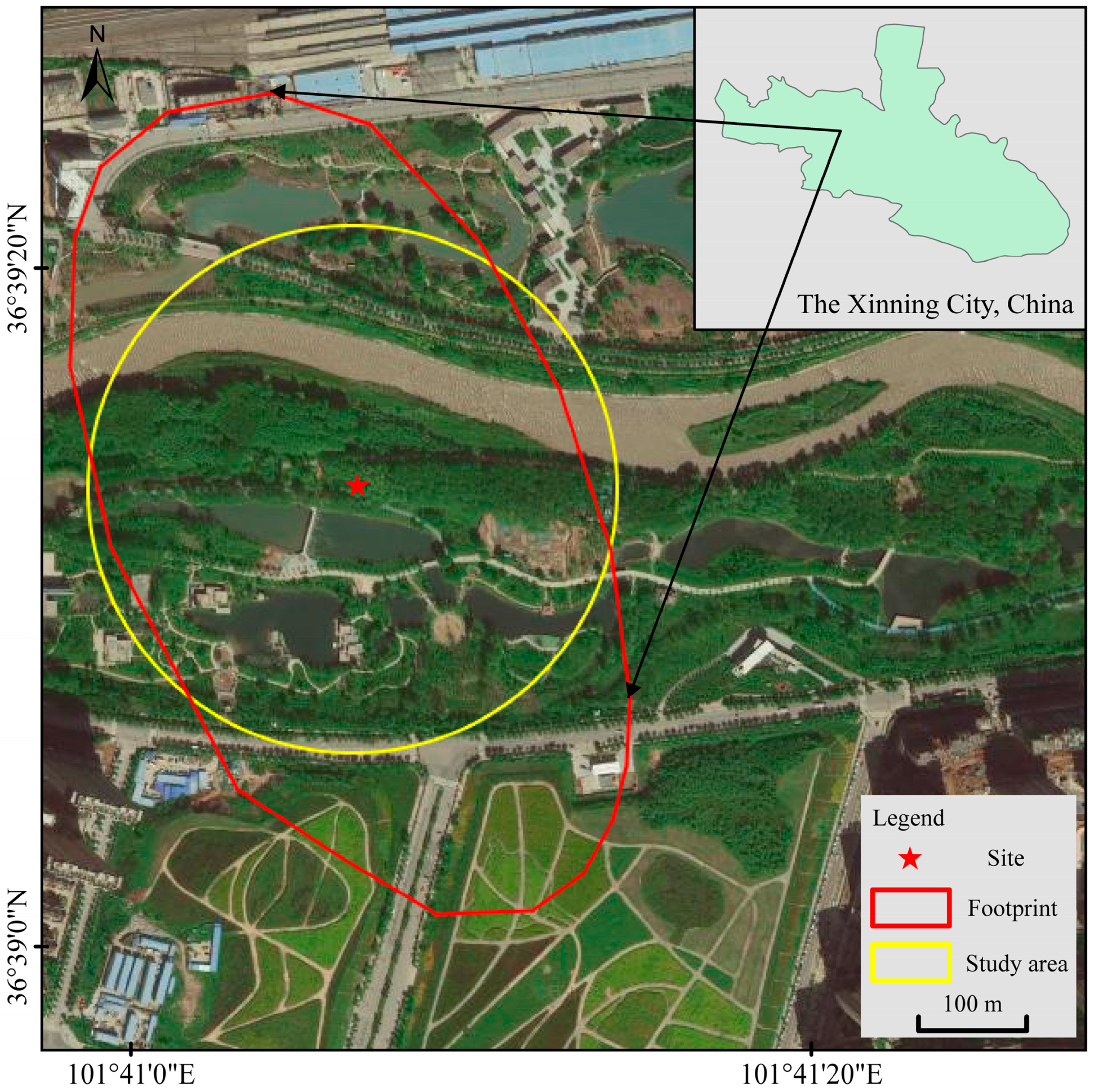
2.1. Description of the Area

The flux tower (36°39′14′′, 101°41′7′′) was located in the Huangshui National Wetland Park, Xining City, Qinghai Province, China. The altitude of this park is about 2290 m. The park has a plateau semi-arid climate with an annual temperature of 5.7 °C, annual precipitation of 360–400 mm, annual evaporation of 1363.6 mm, strong solar radiation, long sunshine time and large temperature difference between day and night [28]. The park has a total area of 5.09 km², and is the largest wetland ecosystem in Xining City. The vegetation covers a large area, dominated by perennial trees which mainly include Populus cathayana Rehd, Salix babylonica and Pinus tabuliformis Carr.

In order to better understand the spatial ranges represented by the observed value of the eddy covariance instrument, in this study, the source area range of the observation tower was calculated using the footprint model (Kljun model) [29], which is relatively new and has been validated. The region surrounded by the 90% horizontal isoline represents the region with a contribution rate of 90% to the value observed. This region is named as the 90% contribution source area. The range of the 90% contribution source area calculated in this paper varied from 125 to 491 m. The range of source areas in the northwest direction (270° to 320°), principally the Huangshui River and artificial wetland water area, exceeds the average value. Additionally, the range of source areas in the southeast direction (120° to 150°), primarily the artificial wetland vegetation area, also exceeds the average value. In contrast, the ranges of source areas in the east and west directions are slightly smaller than average. Therefore, the average range of the 90% contribution source area (246 m) was taken as the radius of the circular study area with the center of the observation point (Figure 1).

2.2. Instrument Setting and Field Observation

The eddy covariance system is mainly composed of an LI-7500RS-type open-circuit three-dimensional ultrasonic anemometer, CSAT3-type open-circuit CO₂/H₂O analyzer, and data collector, with sampling frequency of 10 Hz. The original output data of the 3D ultrasonic anemometer include horizontal wind speed, vertical wind speed, ultrasonic virtual temperature, and the diagnostic value of the instrument. The original output data of the CO₂/H₂O analyzer include the absolute density of CO₂, absolute density of water vapor, intensity of CO₂ signal, and diagnostic value of the instrument. When the eddy covariance system was operated, the CO₂ flux was calculated once every 30 min and the value was stored with the original data observed. The flux results calculated on-line should be calibrated before they are used for scientific research. To ensure the accuracy of the measured CO₂ and H₂O fluxes, the CO₂ and H₂O analyzers were calibrated with standard CO₂ gas (±1% 450 ppm) and a dew-point generator (LI-610) every three months. The 3D anemometer was maintained regularly, and the wind speed measured was compared with the value derived from a micro meteorological station to ensure an error of less than 5%. Soil temperature (T_soil) at a depth of 5 cm underground and soil water content (SWC) were automatically recorded every 30 min via a data collector (Sutron9210 Xlite, USA).

2.3. Eddy Covariance Technology

The CO₂ flux is defined as the quantity of CO₂ transported per unit area in unit time [30], and can be calculated as follows:

$$\mathrm{F}=\overline{w\times r}=\overline{w}\times \overline{r}+\overline{w^{\prime }\times r^{\prime }}$$

(1)

where w represents the vertical component of three-dimensional wind speed (m·s⁻¹); r is the molar concentration of CO₂ measured by the instrument (μmol·m⁻³); w′ and r′ represent the deviations between instantaneous and average values of w and r, respectively. The upper lines indicate the average values in the corresponding periods.

3. Materials and Methods

3.1. Data Quality Control

The original 10 Hz data were processed using the Express module in the Eddypro software (LI-COR Company). The processing steps include coordinate axis rotation correction, trend correction, data synchronization, statistical test, density correction, ultrasonic virtual temperature correction, spectrum correction, attack angle correction, data quality control mark and other procedures. Finally, 30 min of flux data were obtained [31,32,33].

Due to the influence of measurement errors and weather factors, the quality of partial data was poor. Thereby, quality assessment (QA) of the 30-min flux data was required [34]: (1) The abnormal flux values calculated by the EddyPro software were excluded; (2) the flux data obtained in raining and snowing periods were excluded; (3) the poor-quality flux data represented by 2 in the “0–1–2” quality evaluation method of the EddyPro software were excluded.

For the CO₂ flux data derived at night, in addition to the above-mentioned quality control process, the quality control was enhanced as follows: (1) The negative data at night were excluded because only the respiration of vegetation and soil occurred at night; (2) based on data analysis, the empirical threshold of CO₂ flux is 23 μmol·m⁻²·s⁻¹, so the values beyond this threshold were excluded; (3) the instrument response to the weak convection at night was insensitive, so the intensity of air turbulence was evaluated according to the air friction velocity (u*), and the CO₂ flux data with night friction wind speeds lower than 0.2 m·s⁻¹ were excluded; (4) the abnormally large values were excluded, according to the quadruple standard deviation of CO₂ flux value. After the quality control, 41.4% of the original flux data were excluded, and the exclusion rate was greater than that of FLUXNET (35%) [35].

3.2. Data Interpolation

(1) For the day-time, CO₂ flux data of net ecosystem excluded, the Michaaelis–Menten equation was adopted in the interpolation by fitting [36]:

$${\mathrm{NEE}}_{\mathrm{d}}={\mathrm{R}}_{\mathrm{eco},\mathrm{d}}-{\mathrm{P}}_{\max }\times \alpha \times \mathrm{PAR}/\left({\mathrm{P}}_{\max }+\alpha \times \mathrm{PAR}\right)$$

(2)

where NEE_d stands for the CO₂ flux data (mg·m⁻²·s⁻¹) measured by the day-time eddy covariance system; R_eco,d stands for the dark respiration rate of ecosystem during the day (mg·m⁻²·s⁻¹); PAR is the photosynthetically active radiation (μmol·m⁻²·s⁻¹); α is the apparent initial light energy utilization efficiency (mg·μmol⁻¹); P_max stands for the maximum photosynthetic rate (mg·m⁻²·s⁻¹), which is the net photosynthetic rate of the ecosystem corresponding to a maximum PAR value.

(2) For the night-time flux data excluded, the interpolation was performed on the basis of the relationship between CO₂ flux and soil temperature [37]:

$${\mathrm{R}}_{\mathrm{eco},\mathrm{n}}=\mathrm{a}\exp \left(\mathrm{b}{\mathrm{T}}_{\mathrm{soil}}\right)$$

(3)

where R_eco,n stands for the CO₂ flux data measured by the night-time eddy covariance system; a and b are the fitting coefficients; T_soil is the relevant soil temperature.

(3) The temperature sensitivity coefficient of ecosystem respiration (Q₁₀) was calculated by the following equation [38]:

$${\mathrm{Q}}_{10}=\exp \left(10\mathrm{b}\right)$$

(4)

(4) For the conventional meteorological data, when the data were excluded continuously less than four times, the linear interpolation was performed; when the data were excluded continuously more than four times, but less than eight times, the average value of the values observed at the same time in the four days before and after the missing date was taken as the required value. If the data were excluded continuously more than eight times, the average value in the relevant month was taken as the value required [39].

3.3. Split of CO₂ Flux Data

Ecosystem respiration (R_eco) is the basis to calculate the total productivity of the ecosystem (GEP). Since photosynthesis does not take place for plants at night, NEE_n can be taken as the night-time ecosystem respiration (R_eco,n). A respiratory curve can be obtained by fitting models to the flux and temperature data at night, and the daytime ecosystem respiration (R_eco,d) can be obtained by calculating the value corresponding to the daytime temperature according to the respiratory curve [40]. The ecosystem respiration is defined as:

$${\mathrm{R}}_{\mathrm{eco}}={\mathrm{R}}_{\mathrm{eco},\mathrm{d}}+{\mathrm{R}}_{\mathrm{eco},\mathrm{n}}$$

(5)

Therefore, the total primary productivity GPP can be expressed as:

$$\mathrm{GPP}=\mathrm{NEE}-{\mathrm{R}}_{\mathrm{eco}}$$

(6)

At the ecosystem scale, the total ecosystem productivity equals the total primary productivity:

$$\mathrm{GEP}=\mathrm{GPP}$$

(7)

3.4. Data Statistical Analysis

The data were processed using Microsoft Excel 2016 software, and statistical analysis was conducted with IBM SPSS Statistics 25 software. Graphs were made with Origin 2020 software. Data completed by fitting and interpolation were used to analyze the temporal and spatial variation characteristics of CO₂ flux, while only effective data were used to analyze the influence of environmental factors on net CO₂ exchange. The half-hour and daily average fluxes were taken as the arithmetic means in corresponding periods, and the monthly and total fluxes were taken as the cumulative values in corresponding periods.

4. Results

4.1. Daily Dynamic Change of CO₂ Flux

At an interval of half an hour, the monthly average mean of net ecosystem CO₂ exchange (NEE) at the same time of each month was calculated, according to the CO₂ flux data in the warm season (July to September) in 2020, and thus, the month-average daily changes in NEE in different months were obtained (Figure 2). A positive NEE value reflects CO₂ emission, and a negative value correlates to CO₂ uptake. Figure 2 shows that the NEE in the warm season of the wetland exhibited obvious daily variation characteristics, and the daily fluctuation curve is generally in a “U” shape. Carbon uptake (−0.24 ± 0.28 mg·m⁻²·s⁻¹) took place in the daytime while carbon emission occurred at night (0.17± 0.19 mg·m⁻²·s⁻¹). During the study period, the daily CO₂ uptake in July, August, and September occurred at about 8:00, and the NEE gradually changed from positive to negative, indicating that the photosynthetic rate of the ecosystem was higher than that of the respiration rate and carbon emission was altered by carbon uptake. The maximum CO₂ uptake peak took place in the range of 12:00 to 14:00, and the values were −0.62, −0.56, and −0.62 mg·m⁻²·s⁻¹, respectively. Then, the uptake value was gradually weakened, and the carbon uptake was altered by carbon emission at about 18:30. The maximum CO₂ emission peak took place in the range of 22:00 to 23:00, and the values were 0.34, 0.28, and 0.18 mg·m⁻²·s⁻¹. The average daily fluctuation in July is most obvious from −0.62 to 0.34 mg·m⁻²·s⁻¹. Meanwhile, the fluctuations of net CO₂ emissions in the ecosystem at night were relatively small, and the values are significantly smaller than those of the net CO₂ uptake in the daytime (p < 0.01).

4.2. Monthly Dynamic Change of CO₂ Flux

Table 1. CO₂ sink capacity of the plateau urban wetland in the warm season.

Month	GPP Flux mg·m−2·s−1	Reco Flux mg·m−2·s−1	NEE Flux mg·m−2·s−1	CO2 Budget g·m−2·month−1
7	0.30 ± 0.39 a	0.26 ± 0.06 a	−0.04 ± 0.36 a	−102.05
8	0.25 ± 0.36 a	0.21 ± 0.06 b	−0.05 ± 0.34 a	−120.53
9	0.22 ± 0.41 b	0.17 ± 0.29 c	−0.06 ± 0.29 a	−142.82

Note: ^{a, b, c} different letters in the same column indicate significant difference (p < 0.05).

shows the average and cumulative CO₂ fluxes of the plateau urban wetland ecosystem in the warm season (July to September) in 2020. Carbon sink took place in each month of the warm season. Over the measurement period, though the month-average GPP flux and month-average R_eco flux decreased gradually, the difference between them increased month by month. The month-average NEE fluxes in July, August and September were −0.04, −0.05, and −0.06 mg·m⁻²·s⁻¹, respectively. The carbon sink capacity of the wetland ecosystem increased month by month, and the monthly total CO₂ uptake was −102.05, −120.53, and −142.82 g·m⁻²·month⁻¹, respectively.

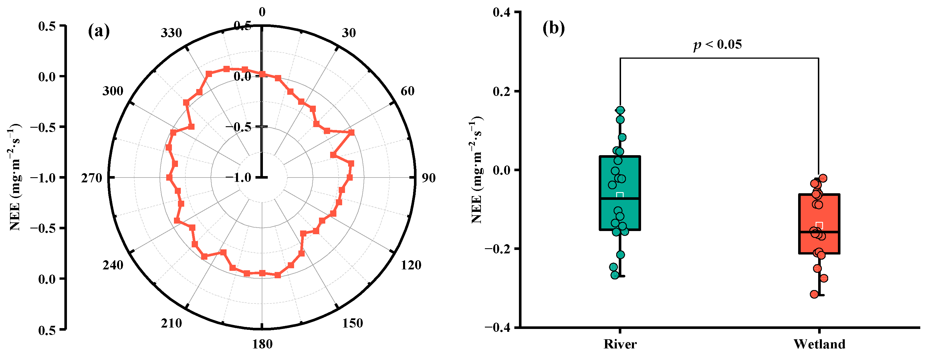
4.3. Spatial Variation of CO₂ Flux

Figure 3a shows the net CO₂ exchange capacities of the plateau urban wetland ecosystem in all wind directions in the warm season, and the flux fluctuated between −0.32 and 0.15 mg·m⁻²·s⁻¹. According to the distribution characteristics of the wetland park, the research area was divided into two parts, with the 90° and 270° wind directions as the boundary. The north and south parts are denoted by river and artificial wetland regions. All the areas with net CO₂ emissions were located in the river area (0–30° and 300–360°), and net CO₂ uptake was found in other wind directions. One-way analysis of variance results (Figure 3b) show that carbon uptake, −0.07 ± 0.03 and −0.14 ± 0.03 mg·m⁻²·s⁻¹, occurred in both regions during the whole study period, but the carbon uptake intensity of the artificial wetland area was significantly higher than that of the river region (p < 0.05).

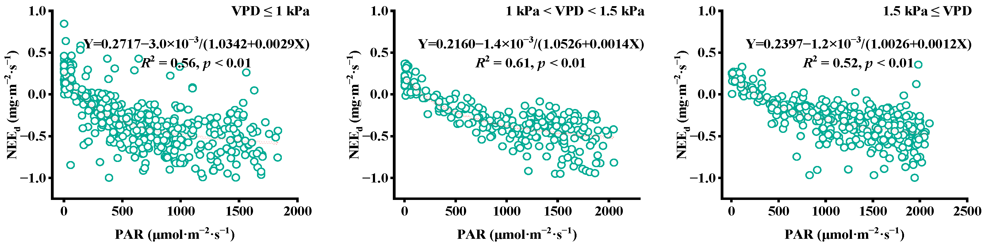
4.4. Factors Affecting CO₂ Flux

For a better understanding of the response of flux characteristics to environmental factors, the net CO₂ exchange capacity in the warm season can be split into day-time (NEE_d) and night-time (NEE_n).

Table 2. The Pearson correlation coefficients between NEE and environmental factors.

Time	PAR	Tsoil	Tair	VPD	SWC
Daytime	−0.446 **	0.140	0.098 **	0.186 **	−0.064
Night	−0.032	0.213 **	0.097	0.114	−0.231 **

Note: ** p < 0.01.

shows the Pearson correlation coefficients between NEE and primary environmental factors in a typical sunny day at a 0.5-h scale. During the day, NEE_d was significantly negatively correlated (p < 0.01) with photosynthetically active radiation (PAR) and significantly positively correlated (p < 0.01) with the saturated vapor pressure difference (VPD) and air temperature (T_air). At night, NEE_d was significantly positively correlated (p < 0.01) with soil temperature (T_soil) and significantly negatively correlated (p < 0.01) with soil moisture content (SWC).

5. Discussion

5.1. Factors Affecting Daytime CO₂ Flux

Photosynthetically active radiation directly affects the photosynthesis of plants and is a major environmental factor affecting the net CO₂ exchange of the ecosystem in the daytime [41]. In this study, the Michaelis–Menten equation was adopted to correlate NEE_d and PAR (Equation (2)). Figure 4a shows that NEE_d and PAR obviously exhibited a rectangular hyperbola relationship on the daily scale. With an increase in PAR, NEE_d decreased significantly (p < 0.01), indicating that the carbon sink capacity of the wetland was significantly enhanced due to the strengthened photosynthetically active radiation. Meanwhile, the influence of PAR on NEE_d in different months (Figure 4b) was studied (Figure 4b). The results show that the apparent quantum efficiency (α), parameter of maximum photosynthetic rate (P_max), and dark respiration rate of the ecosystem in daytime (R_eco,d) displayed season-dependent trends: in the warm season of 2020, the maximum α value of the plateau urban wetland ecosystem was registered in August, and P_max and R_eco,d reached their maximums in July. Approximately 64% of the changes in NEE_d during the study period can be ascribed to PAR, which indicates that PAR is the key environmental factor affecting NEE_d. However, NEE_d cannot be predicted by PAR alone, and is also largely affected by other environmental factors (Table 2).

The saturated vapor pressure difference determines the canopy conductance and closure degree of plant leaf stomas; thus, affecting the photosynthetic capacities of trees [42,43]. Based on the analysis of the response processes of plateau urban wetland NEE_d to PAR under different VPD conditions (Figure 5), it was found that under three VPD conditions, pronounced rectangular hyperbola relationships between PAR and NEE_d were observed. When the VPD was ≤ 1 kPa, most of the corresponding photosynthetically active radiation was weak, and the light saturation point could not be readily reached for the photosynthesis of plant leaves. At this time, R_eco,d reached its maximum of 0.2717 mg·m⁻²·s⁻¹. The values α, P_max, and R² were 0.0029 mg·μmol⁻¹, 1.0342 mg·m⁻²·s⁻¹, and 0.56. When VPD was in the range of 1 to 1.5 kPa, α decreased, while P_max and R² increased. When P_max reached the maximum value of 1.0526 mg·μmol⁻¹, the photosynthesis efficiency of the ecosystem also reached the maximum. When VPD was ≥ 1.5 kPa, the stomas were partially closed and P_max decreased, so VPD tended to inhibit the photosynthesis of ecosystem. In summary, excessively high and low VPD values were not conducive to the photosynthesis of plants, and the VPD range of 1–1.5 kPa is most suitable for the photosynthesis of vegetation in plateau urban wetlands. In addition, on the one hand, T_air had an indirect impact on the stomas of plant leaves by affecting the VPD, resulting in a light saturation phenomenon and thereby changing the net photosynthetic rate dynamics [44]. On the other hand, excessively high T_air directly destructed the cellular structures of leaves, and passivated the enzymes for photosynthesis, thus, affecting the net photosynthetic rate [42]. Nonetheless, the regression analysis results show that T_air and NEE_d were linearly correlated, but the relationship was weak (R² = 0.09), indicating that T_air was not the major factor limiting the daytime photosynthesis.

5.2. Factors Influencing CO₂ Flux at Night

Temperature, as one of the important driving forces of ecosystem respiration, has a significant impact on carbon exchange in night ecosystems. Especially in high-altitude regions, the temperatures change greatly between day and night and among seasons, so temperature is often a major environmental factor controlling the CO₂ flux [37,45,46]. Therefore, the NEE_n was correlated with soil temperature at a depth of 5 cm underground. The NEE_n refers to the average CO₂ flux in half an hour, corresponding to an interval of 0.5 °C. The fitting results are shown in Figure 6a. With the increase in T_soil, the NEE_n of urban wetland ecosystem in the warm season increased exponentially (R² = 0.88), indicating that the soil temperature could be the reason for the respiration variation of the ecosystem at night. Different from other regions, in the Qinghai–Tibet Plateau, the biogeochemical activities of various organisms adapt to the regional environment, and usually take place under extremely cold conditions, so slight changes in temperature will cause evident changes in their activities [47]. Q₁₀ is a sensitivity parameter used to depict the response of CO₂ flux to temperature variation, and it is defined as the increasing fold of CO₂ flux corresponding to 10 ℃ of temperature rise [48]. The soil temperature at 5 cm corresponded to a Q₁₀ value of 2.48, within the Q₁₀ range of 1.28 to 4.75 for the land ecosystems in China [49]. This is lower than the value (3.45) of alpine meadow wetlands in the Qinghai–Tibet Plateau [50], yet far higher than that (1.33) of the Yellow River Estuary intertidal salt marsh wetland [51] and that (1.84) of the Shenlongjia Dajiu Lake peat wetland [52]. In conclusion, the response of the CO₂ flux of plateau urban wetland ecosystem to the change in soil temperature is relatively sensitive, which indicates that more attention should be paid in the situation of global warming.

Soil water content affects the NEE_n by changing the oxygen content in the soil and redox potential of the wetland ecosystem. Ultra-high or ultra-low SWC values will limit the respiration of soil organisms [53]. During the study period, the SWC value at night of the plateau urban wetland varied in the range of 21.03–28.49%. The average CO₂ flux in half an hour was correlated to SWC values at intervals of 5% following the binomial fitting. The results are shown in Figure 6b (R² = 0.83). With the increase in SWC, NEE_n increased. When SWC reached 21.64%, NEE_n reached the maximum. Then, with the increase in SWC, NEE_n decreased, indicating that the optimal soil moisture content that is favorable for the carbon emission of plateau urban wetland is around 21.64%.

5.3. Importance and Particularity of CO₂ Fluxes of Plateau Urban Wetlands in Warm Seasons

Urban wetland plays an important role in global carbon cycle through carbon fixation and oxygen release, and has a high value of climate regulation [7,28]. As the Qinghai–Tibet Plateau is located in a high-altitude area, the climate does not change obviously among the four seasons, showing obvious cold and warm seasons [54]. Compared to the long cold season, the rainy and thermal warm season plays an important role in the carbon cycle of urban wetland ecosystem in the Qinghai–Tibet Plateau, and is the main period for the fast growing of vegetation and CO₂ uptake. During the study period, the overall CO₂ uptake of −365.40 g·m⁻² in the study area was observed, and this value is comparable to that of the Artemisia selengensis meadow wetland in Qinghai Lake (−351.14 g·m⁻²) [47], and higher than that of the low-altitude Yellow River Delta reed wetland (−195.39 g·m⁻²) and the salt marsh wetland (−81.69 g·m⁻²) [51,55], indicating that the urban wetland ecosystem of the Qinghai–Tibet Plateau is an important carbon sink. Similar to other ecosystems, the NEE showed obvious daily changes in the warm season. The daily flux maximum of CO₂ uptake in the plateau urban wetland ecosystem reached 0.62 mg·m⁻²·s⁻¹, comparable to that of the alpine meadow wetland in the eastern margin of the Qinghai–Tibet Plateau (0.68 mg·m⁻²·s⁻¹) [50], higher than that of the Artemisia selengensis meadow wetland (0.42 mg·m⁻²·s⁻¹) [47] and cold wetland of the source region of the Yellow River (0.55 mg·m⁻²·s⁻¹) [46], and lower than that of the cold Maqu meadow wetland (10.20 mg·m⁻²·s⁻¹) [56]. Compared to the wetland ecosystems in the plain area, the value is higher than that of the Shenlongjia Dajiu Lake peat wetland (0.30 mg·m⁻²·s⁻¹) [52] and lower than that of the unflooded Nanji wetland of Poyang Lake (0.80 mg·m⁻²·s⁻¹) [6]. In the warm season, solar radiation in the northeast of the Qinghai–Tibet Plateau is strong, and the temperature difference between day and night is large, so the daily CO₂ flux varied between −0.62 and 0.34 mg·m⁻²·s⁻¹, to a larger extent. The fluctuation is larger than that of the peat swamp in the Canada estuary (−0.29–0.18 mg·m⁻²·s⁻¹) [57], yet smaller than that of the reed wetland in Northeast China (−1.0–0.30 mg·m⁻²·s⁻¹) [58] and the Amazon marsh wetland (−0.88–0.30 mg·m⁻²·s⁻¹) [59].

Plateau urban wetlands are usually constructed in the vicinity of rivers, and the close material circulation and energy flow between them will inevitably lead to dynamic changes in the source and sink functions of wetlands. Due to the particularity of plateau rivers, in the global carbon cycle, rivers not only play the role of a “pipeline” connecting land and marine ecosystems, but are also important greenhouse gas emission sources [60]. It has been reported that urban rivers, affected by humans, have higher greenhouse gas emissions. For example, eutrophication can change the structure and function of the ecosystem, thus, affecting the dynamic emission of greenhouse gases [61]. Due to the existence of rivers, some of the regions in the plateau urban wetland ecosystem exhibited net CO₂ emissions, and the CO₂ uptake intensity in the wetland region was significantly higher than that in the river region. In addition, the warming trend of the Qinghai–Tibet Plateau is becoming more and more obvious under the influence of global warming, and the warming rate in the past 40 years is twice the global average rate in the same period [62,63]. High temperatures, increased eutrophication, and their interaction can significantly affect the production, transportation, and emission of greenhouse gases [64]. Under the dual actions of global climate change and human activities, the source and sink effects of the plateau urban wetland ecosystem face many challenges, and more attention should be paid to this issue in the future.

6. Conclusions

With the development of warming changes in the global climate, the uncertainty related to greenhouse gas emissions from the Qinghai–Tibet Plateau wetlands, especially the urban wetlands, has increased significantly. In this study, the Huangshui National Wetland in Xining City, Qinghai–Tibet Plateau, which is sensitive to climate change and human activities, was taken as the research object. The temporal and spatial variation characteristics and influencing factors of CO₂ flux in the warm season (July to September 2020) were analyzed. The principal conclusions are presented as follows:

(1) The CO₂ flux of urban wetland ecosystem in the Qinghai–Tibet Plateau exhibited obvious “U” type daily change characteristics. CO₂ uptake was observed in the daytime and emission was recorded at night, with a large daily variation range.

(2) The urban wetland ecosystem of the Qinghai–Tibet Plateau had a strong carbon sink function in the warm season, with total uptake of −365.40 g·m⁻². However, due to the net CO₂ emission in some river regions, the carbon uptake intensity of the artificial wetland region was significantly higher than that of the river region.

(3) During the day, the CO₂ flux was primarily affected by PAR and VPD, and the optimal VPD, which was most favorable for the carbon uptake of ecosystem, was in the range of 1–1.5 kPa. At night, the CO₂ flux was largely affected by T_soil and SWC, and the optimal SWC, which was most favorable for the carbon emission of ecosystem, was 21.64%.

This is noteworthy because the research object is located in the city, large quantities of C, N and other nutrients have been discharged into the object, and these nutrients will change the structure and function of the ecosystem through eutrophication, and thereby noticeably affect the emission dynamics of CO₂, especially CO₂ emission from rivers. Therefore, monitoring factors related to the water environment, such as dissolved oxygen, dissolved organic carbon, and total nitrogen, should be enhanced in the future. In addition, methane emission should be assessed in future studies, so the carbon budget of the plateau urban wetland ecosystem can be evaluated with higher precision.

References

1. Chen, Q.; Guo, B.; Zhao, C.; Xing, B. Characteristics of CH4 and CO2 emissions and influence of water and salinity in the Yellow River delta wetland, China. Environ. Pollut. 2018, 239, 289–299. [Google Scholar] [CrossRef]
2. Xiao, S.; Wang, Y.; Liu, D.; Yang, Z.; Lei, D.; Zhang, C. Diel and seasonal variation of methane and carbon dioxide fluxes at Site Guojiaba, the Three Gorges Reservoir. J. Environ. Sci. 2013, 25, 2065–2071. [Google Scholar] [CrossRef]
3. Yang, D.X.; Mao, X.F.; Wei, X.Y.; Tao, Y.Q.; Zhang, Z.F.; Ma, J.H. Water-air interface greenhouse gas emissions (CO2, CH4, and N2O) emissions were amplified by continuous dams in an urban river in Qinghai–Tibet Plateau, China. Water 2020, 12, 759. [Google Scholar] [CrossRef] [Green Version]
4. Mao, X.; Wei, X.; Engel, B.; Wei, X.; Zhang, Z.; Tao, Y.; Wang, W. Network-based perspective on water-air interface GHGs flux on a cascade surface-flow constructed wetland in Qinghai-Tibet Plateau, China. Ecol. Eng. 2020, 151, 105862. [Google Scholar] [CrossRef]
5. Mao, X.; Wei, X.; Engel, B.; Wang, W.; Jin, X.; Jin, Y. Biological response to 5 years of operations of cascade rubber dams in a plateau urban river, China. River Res. Appl. 2020. [Google Scholar] [CrossRef]
6. Wang, L.L.; Yang, T.; Gao, C.; Gao, D.; Lu, C.F.; Wang, Y.Q. Diurnal Variation of Net Ecosystem CO2 Exchange of Nanji Wetland Ecosystem in Poyang Lake. J. Ecol. Rural Environ. 2017, 33, 1007–1012. [Google Scholar] [CrossRef]
7. Yang, Y.P.; Cao, G.Z.; Hou, P.; Jiang, W.G.; Chen, Y.H.; Li, J. Monitoring and evaluation for climate regulation service of urban wetlands with remote sensing. Geogr. Res. 2013, 32, 73–80. [Google Scholar] [CrossRef]
8. Smith, R.M.; Kaushal, S.S.; Beaulieu, J.J.; Pennino, M.J.; Welty, C. Influence of infrastructure on water quality and greenhouse gas dynamics in urban streams. Biogeosciences 2017, 14, 2831–2849. [Google Scholar] [CrossRef] [Green Version]
9. Borges, A.V.; Darchambeau, F.; Lambert, T.; Morana, C.; Allen, G.H.; Tambwe, E.; Toengaho Sembaito, A.; Mambo, T.; Nlandu Wabakhangazi, J.; Descy, J.P. Variations in dissolved greenhouse gases (CO2, CH4, N2O) in the Congo River network overwhelmingly driven by fluvial-wetland connectivity. Biogeosciences 2019, 16, 3801–3834. [Google Scholar] [CrossRef] [Green Version]
10. Maucieri, C.; Barbera, A.C.; Vymazal, J.; Borin, M. A review on the main affecting factors of greenhouse gases emission in constructed wetlands. Agric. For. Meteorol. 2017, 236, 175–193. [Google Scholar] [CrossRef]
11. Nuamah, L.A.; Li, Y.P.; Pu, Y.S.; Nwankwegu, A.S.; Haikuo, Z.; Norgbey, E.; Banahene, P.; Bofah-Buoh, R. Constructed wetlands, status, progress, and challenges. The need for critical operational reassessment for a cleaner productive ecosystem. J. Clean. Prod. 2020, 269, 122340. [Google Scholar] [CrossRef]
12. Badiou, P.; Page, B.; Ross, L. A comparison of water quality and greenhouse gas emissions in constructed wetlands and conventional retention basins with and without submerged macrophyte management for storm water regulation. Ecol. Eng. 2019, 127, 292–301. [Google Scholar] [CrossRef]
13. Ma, J.J.; Ullah, S.; Niu, A.; Liao, Z.N.; Qin, Q.H.; Xu, S.J.; Lin, C.X. Heavy metal pollution increases CH4 and decreases CO2 emissions due to soil microbial changes in a mangrove wetland: Microcosm experiment and field examination. Chemosphere 2021, 269, 128735. [Google Scholar] [CrossRef] [PubMed]
14. Li, X.F.; Sardans, J.; Hou, L.J.; Liu, M.; Xu, C.B.; Peñuelas, J. Climatic temperature controls the geographical patterns of coastal marshes greenhouse gases emissions over China. J. Hydrol. 2020, 590, 125378. [Google Scholar] [CrossRef]
15. Yu, G.R.; Sun, X.M. Principles of Flux Measurement in Terrestrial Ecosystems; Higher Education Press: Beijing, China, 2006; pp. 40–44. [Google Scholar]
16. Li, G.D.; Zhang, J.H.; Chen, C.; Tian, H.F.; Zhao, L.P. Research progress on carbon storage and flux in different terrestrial ecosystem in China under globa climate change. Ecol. Environ. Sci. 2013, 22, 873–878. [Google Scholar] [CrossRef]
17. Liang, A.L. Research of Space-Borne Remote Sensing for Carbon Dioxide on Validation, Inversion and Application. Ph.D. Thesis, WUHAN University, Wuhan, China, 2018. [Google Scholar]
18. Stagakis, S.; Chrysoulakis, N.; Spyridakis, N.; Feigenwinter, C.; Vogt, R. Eddy Covariance measurements and source partitioning of CO2 emissions in an urban environment: Application for Heraklion, Greece. Atmos. Environ. 2019, 201, 278–292. [Google Scholar] [CrossRef]
19. Baldocchi, D. Assessing ecosystem carbon balance: Problems and prospects of the eddy covariance technique. Glob. Chang. Biol. 2003, 9, 478–492. [Google Scholar] [CrossRef] [Green Version]
20. Chen, S.P.; You, C.H.; Hu, Z.M.; Chen, Z.; Zhang, L.M.; Wang, Q.F. Eddy covariance technique and its applications in flux observations of terrestrial ecosystems. Chin. J. Plant Ecol. 2020, 44, 291–304. [Google Scholar] [CrossRef]
21. Richardson, A.D.; Hollinger, D.Y.; Shoemaker, J.K.; Hughes, H.; Savage, K.; Davidson, E.A. Six years of ecosystem-atmosphere greenhouse gas fluxes measured in a sub-boreal forest. Sci. Data 2019, 6, 117. [Google Scholar] [CrossRef] [Green Version]
22. Liu, W.T.; Yao, X.L.; Xue, J.Y.; Zhao, Z.H.; Zhang, L.; Wang, X.L.; Cai, Y.J. Seasonal and Spatial Variations in Greenhouse Gases(CH4 and CO2) Emission Along the Riparian Zone of Middle and Lower Reaches of Yangtze River. Resour. Environ. Yangtze Basin 2019, 28, 2718–2726. [Google Scholar] [CrossRef]
23. Wei, S.; Han, G.; Jia, X.; Song, W.; Chu, X.; He, W.; Xia, J.; Wu, H. Tidal effects on ecosystem CO2 exchange at multiple timescales in a salt marsh in the Yellow River Delta. Estuarine, Coast. Shelf Sci. 2020, 238, 106727. [Google Scholar] [CrossRef]
24. Attermeyer, K.; Flury, S.; Jayakumar, R.; Fiener, P.; Steger, K.; Arya, V.; Wilken, F.; van Geldern, R.; Premke, K. Invasive floating macrophytes reduce greenhouse gas emissions from a small tropical lake. Sci. Rep. 2016, 6, 20424. [Google Scholar] [CrossRef]
25. Immerzeel, W.W.; van Beek, L.P.H.; Bierkens, M.F.P. Climate Change Will Affect the Asian Water Towers. Science 2010, 328, 1382–1385. [Google Scholar] [CrossRef]
26. Lang, Q.; Niu, Z.G.; Hong, X.Q.; Yang, X.Y. Remote Sensing Monitoring and Change Analysis of Wetlands in the Tibetan Plateau. Geomat. Inf. Sci. Wuhan Univ. 2021, 46, 230–237. [Google Scholar] [CrossRef]
27. Meng, W.Q.; He, M.X.; Hu, B.B.; Mo, X.Q.; Li, H.Y.; Liu, B.Q.; Wang, Z.L. Status of wetlands in China: A review of extent, degradation, issues and recommendations for improvement. Ocean Coast. Manag. 2017, 146, 50–59. [Google Scholar] [CrossRef]
28. Mao, X.F.; Wei, X.Y.; Chen, Q.; Liu, F.G.; Tao, Y.Q.; Zhang, Z.F. An ECPS framework based assessment on wetland restoration of the Huangshui National Wetland Park in Qinghai Province, China. Geogr. Res. 2019, 38, 760–771. [Google Scholar] [CrossRef]
29. Kljun, N.; Calanca, P.; Rotach, M.W.; Schmid, H.P. A simple two-dimensional parameterisation for Flux Footprint Prediction (FFP). Geosci. Model Dev. 2015, 8, 3695–3713. [Google Scholar] [CrossRef] [Green Version]
30. Veenendaal, E.; Kolle, O.; Lloyd, J. Seasonal variation in energy fluxes and carbon dioxide exchange for a boad-leaved semi-arid savanna (Mopane Woodland) in Southern Africa. Glob. Chang. Biol. 2003, 10, 318–328. [Google Scholar] [CrossRef]
31. McDermitt, D.; Burba, G.; Xu, L.; Anderson, T.; Komissarov, A.; Riensche, B.; Schedlbauer, J.; Starr, G.; Zona, D.; Oechel, W. A new low-power, open-path instrument for measuring methane flux by eddy covariance. Appl. Phys. B Lasers Opt. 2011, 102, 391–405. [Google Scholar] [CrossRef]
32. Mahrt, L.; Vickers, D. Relationship of area-averaged carbon dioxide and water vapour fluxes to atmospheric variables. Agric. For. Meteorol. 2002, 112, 195–202. [Google Scholar] [CrossRef]
33. Webb, E.K.; Pearman, G.I.; Leuning, R. Correction of flux measurements for density effects due to heat and water-vapor transfer. Q. J. R. Meteorol. Soc. 1980, 106, 85–100. [Google Scholar] [CrossRef]
34. Liu, Y.P.; Li, S.S.; Lü, S.H.; Ao, Y.H.; Gao, Y.H. Comparison of Flux Correction Methods for Eddy-Covariance Measurement. Plateau Meteorol. 2013, 32, 1704–1711. [Google Scholar] [CrossRef]
35. Falge, E.; Baldocchi, D.; Olson, R.; Anthoni, P.; Aubinet, M.; Bernhofer, C.; Burba, G.; Ceulemans, R.; Clement, R.; Dolman, H. Gap filling strategies for defensible annual sums of net ecosystem exchange. Agric. For. Meteorol. 2001, 107, 43–69. [Google Scholar] [CrossRef] [Green Version]
36. Ruimy, A.; Jarvis, P.G.; Baldocchi, D.D.; Saugier, B. CO2 Fluxes over Plant Canopies and Solar Radiation: A Review. Advances in Ecological Research. 1995, 26, 1–68. [Google Scholar] [CrossRef]
37. Lloyd, J.; Taylor, J.A. On the Temperature Dependence of Soil Respiration. Funct. Ecol. 1994, 8, 315–323. [Google Scholar] [CrossRef]
38. Yang, J.F.; Yang, X.N.; Wang, J.H.; Duan, Y.M.; Qi, X.N.; Zhang, L.S. Characteristics of CO2 Flux in a Mature Apple (Malus demestica) Orchard Ecosystem on the Loess Plate. Environ. Sci. 2018, 39, 2339–2350. [Google Scholar] [CrossRef]
39. Hinojo-Hinojo, C.; Castellanos, A.E.; Rodriguez, J.C.; Delgado-Balbuena, J.; Romo-León, J.R.; Celaya-Michel, H.; Huxman, T.E. Carbon and Water Fluxes in an Exotic Buffelgrass Savanna. Rangel. Ecol. Manag. 2016, 69, 334–341. [Google Scholar] [CrossRef]
40. Li, Z.H.; Luo, W.J.; Du, H.; Song, T.Q.; Peng, H.J.; Wang, Y.W.; Wang, S.J. CO2 Flux and Its Driving Factors in a Karst Evergreen Deciduous Broadleaf Mixed Forest in Dry Season. Earth Environ. 2020, 48, 525–536. [Google Scholar] [CrossRef]
41. Zhao, H.C.; Jia, G.S.; Wang, H.S.; Zhang, A.Z.; Xu, X.Y. Diurnal Variations of the Carbon Fluxes of Semiarid Meadow Steppe and Typical Steppe in China. Clim. Environ. Res. 2020, 25, 172–184. [Google Scholar] [CrossRef]
42. Anthoni, P.M.; Law, B.E.; Unsworth, M.H. Carbon and water vapor exchange of an open-canopied ponderosa pine ecosystem. Agric. For. Meteorol. 1999, 95, 151–168. [Google Scholar] [CrossRef]
43. Tan, L.P.; Liu, S.X.; Mo, X.G.; Yang, L.H.; Lin, Z.H. Environmental controls over energy, water and carbon fluxes in a plantation in Northern China. Chin. J. Plant Ecol. 2015, 39, 773–784. [Google Scholar] [CrossRef]
44. Jarvis, P.; Morison, J. The Control of Transpiration and Photosynthesis by the Stomata; Cambridge University Press: Cambridge, UK, 1981; Volume 8, pp. 247–279. [Google Scholar]
45. Huxman, T.E.; Turnipseed, A.A.; Sparks, J.P.; Harley, P.C.; Monson, R.K. Temperature as a control over ecosystem CO2 fluxes in a high-elevation, subalpine forest. Oecologia 2003, 134, 537–546. [Google Scholar] [CrossRef]
46. Luo, Q.; Wen, J.; Wang, X.; Tian, H.; Wang, Z.L. Analysis of the Diurnal Characteristics of Water and Heat & CO2 Exchanges at the Alpine Wetland in the Source Region of the Yellow River. Plateau Meteorol. 2017, 36, 667–674. [Google Scholar] [CrossRef]
47. Wu, F.T.; Cao, S.K.; Cao, G.C.; Han, G.Z.; Lin, Y.Y.; Cheng, S.Y. Variation of CO2 Flux of Alpine Wetland Ecosystem of Kobresia tibetica Wet Meadow in Lake Qinghai. J. Ecol. Rural Environ. 2018, 34, 124–131. [Google Scholar] [CrossRef]
48. Davidson, E.A.; Janssens, I.A.; Luo, Y.Q. On the variability of respiration in terrestrial ecosystems: Moving beyond Q10. Glob. Chang. Biol. 2006, 12, 154–164. [Google Scholar] [CrossRef]
49. Zhan, X.Y.; Yu, G.R.; Zheng, Z.M.; Wang, Q.F. Carbon Emission and Spatial Pattern of Soil Respiration of Terrestrial Ecosystems in China: Based on Geostatistic Estimation of Flux Measurement. Prog. Geogr. 2012, 31, 97–108. [Google Scholar] [CrossRef]
50. Wang, H.B.; Ma, M.G.; Wang, X.F.; Tan, J.L.; Gen, L.Y.; Yu, W.P.; Jia, S.Z. Carbon flux variation characteristics and its influencing factors in an alpine meadow ecosystem on eastern Qinghai-Tibetan plateau. J. Arid Land Resour. Environ. 2014, 28, 50–56. [Google Scholar] [CrossRef]
51. Xing, Q.H.; Han, G.X.; Yu, J.B.; Wu, L.X.; Qiong, Y.L.; Mao, P.L.; Wang, G.M.; Xie, B.H. Net ecosystem CO2 exchange and its controlling factors during the growing season in an inter-tidal salt marsh in the Yellow River Estuary, China. Acta Ecol. Sin. 2014, 34, 4966–4979. [Google Scholar] [CrossRef] [Green Version]
52. Peng, F.J.; Ge, J.W.; Li, Y.Y.; Li, J.Q.; Zhou, Y.; Zhang, Z.Q. Characteristics of CO2 Flux and Their Effect Factors in Dajiuhu Peat Wetland of Shennongjia. Ecol. Environ. Sci. 2017, 26, 453–460. [Google Scholar] [CrossRef]
53. Špunda, V.; Kalina, J.; Urban, O.; Luis, V.C.; Sibisse, I.; Puértolas, J.; Šprtová, M.; Marek, M.V. Diurnal dynamics of photosynthetic parameters of Norway spruce trees cultivated under ambient and elevated CO2: The reasons of midday depression in CO2 assimilation. Plant Sci. 2005, 168, 1371–1381. [Google Scholar] [CrossRef]
54. Chen, D.L.; Xu, B.Q.; Yao, T.D.; Guo, Z.T.; Cui, P.; Chen, F.H.; Zhang, R.H.; Zhang, X.Z.; Zhang, Y.L.; Fan, J. Assessment of past, present and future environmental changes on the Tibetan Plateau. Chin. Sci. Bull. 2015, 60, 3025–3035. [Google Scholar] [CrossRef]
55. Li, Y.; Kang, X.M.; Hao, Y.B.; Ding, K.; Wang, Y.F.; Cui, X.Y.; Mei, X.R. Carbon, water and heat fluxes of a reed (Phragmites australis) wetland in the Yellow River Delta, China. Acta Ecol. Sin. 2014, 34, 4400–4411. [Google Scholar] [CrossRef] [Green Version]
56. Zhang, Y.; Wen, X.H.; Wang, S.Y.; Shang, L.Y.; Zhang, Y. Analysis of the near-surface micrometeorology and CO2 flux over the Maqu alpine meadow in summer. J. Glaciol. Geocryol. 2019, 41, 54–63. [Google Scholar] [CrossRef]
57. D′Acunha, B.; Morillas, L.; Black, T.A.; Christen, A.; Johnson, M.S. Net Ecosystem Carbon Balance of a Peat Bog Undergoing Restoration: Integrating CO2 and CH4 Fluxes From Eddy Covariance and Aquatic Evasion With DOC Drainage Fluxes. J. Geophys. Res. Biogeosci. 2019, 124, 884–901. [Google Scholar] [CrossRef] [Green Version]
58. Li, X.L.; Jia, Q.Y.; Liu, J.M. Seasonal variations in heat and carbon dioxide fluxes observed over a reed wetland in northeast China. Atmos. Environ. 2016, 127, 6–13. [Google Scholar] [CrossRef]
59. Griffis, T.J.; Roman, D.T.; Wood, J.D.; Deventer, J.; Fachin, L.; Rengifo, J.; Del Castillo, D.; Lilleskov, E.; Kolka, R.; Chimner, R.A. Hydrometeorological sensitivities of net ecosystem carbon dioxide and methane exchange of an Amazonian palm swamp peatland. Agric. For. Meteorol. 2020, 295, 108167. [Google Scholar] [CrossRef]
60. Zhang, L.W.; Xia, X.H.; Liu, S.D.; Zhang, S.B.; Li, S.L.; Wang, J.F.; Wang, G.Q.; Gao, H.; Zhang, Z.R.; Wang, Q.R. Significant methane ebullition from alpine permafrost rivers on the East Qinghai-Tibet Plateau. Nat. Geosci. 2020, 13, 349–354. [Google Scholar] [CrossRef]
61. Marescaux, A.; Thieu, V.; Garnier, J. Carbon dioxide, methane and nitrous oxide emissions from the human-impacted Seine watershed in France. Sci. Total Environ. 2018, 643, 247–259. [Google Scholar] [CrossRef]
62. Yao, T.D. A comprehensive study of Water-Ecosystem-Human activities reveals unbalancing Asian Water Tower and accompanying potential risks. Chin. Sci. Bull. 2019, 64, 2761–2762. [Google Scholar] [CrossRef] [Green Version]
63. Zhu, L.P.; Ju, J.T.; Qiao, B.J.; Yang, R.M.; Liu, C.; Han, B.P. Recent lake changes of the Asia Water Tower and their climate response: Progress, problems and prospects. Chin. Sci. Bull. 2019, 64, 2796–2806. [Google Scholar] [CrossRef] [Green Version]
64. Davidson, T.A.; Audet, J.; Jeppesen, E.; Landkildehus, F.; Lauridsen, T.L.; Søndergaard, M.; Syväranta, J. Synergy between nutrients and warming enhances methane ebullition from experimental lakes. Nat. Clim. Chang. 2018, 8, 156–160. [Google Scholar] [CrossRef]
Figure 1. Map of the study area.
Water 13 01176 g001
Figure 2. Month-average daily changes of net ecosystem exchange (NEE).
Water 13 01176 g002
Figure 3. (a): NEE in each wind direction. (b): NEE in river and artificial wetland regions.
Water 13 01176 g003
Figure 4. (a): The relationship between NEEd and PAR. (b): Monthly variation of the light response equation parameters.
Water 13 01176 g004
Figure 5. The relationship between NEEd and PAR under the different VPD.
Water 13 01176 g005
Figure 6. (a): The relationship between NEEn and Soil temperature. (b): The relationship between NEEn and soil water content.
Water 13 01176 g006