
Exploring Artificial Intelligence Techniques for Groundwater Quality Assessment


 , ,
, ,
Abstract
1. Introduction
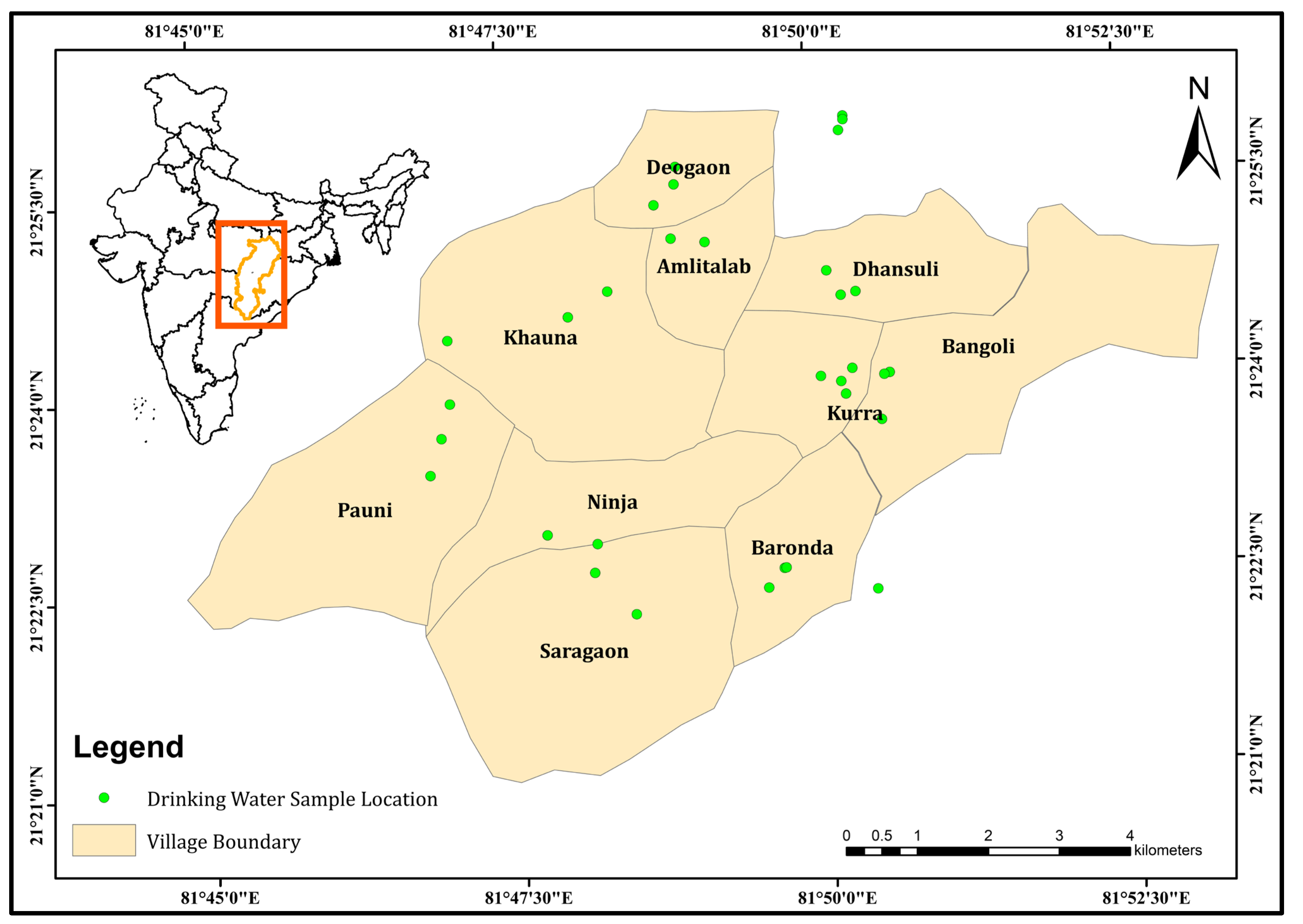
2. Study Area
3. Methodology
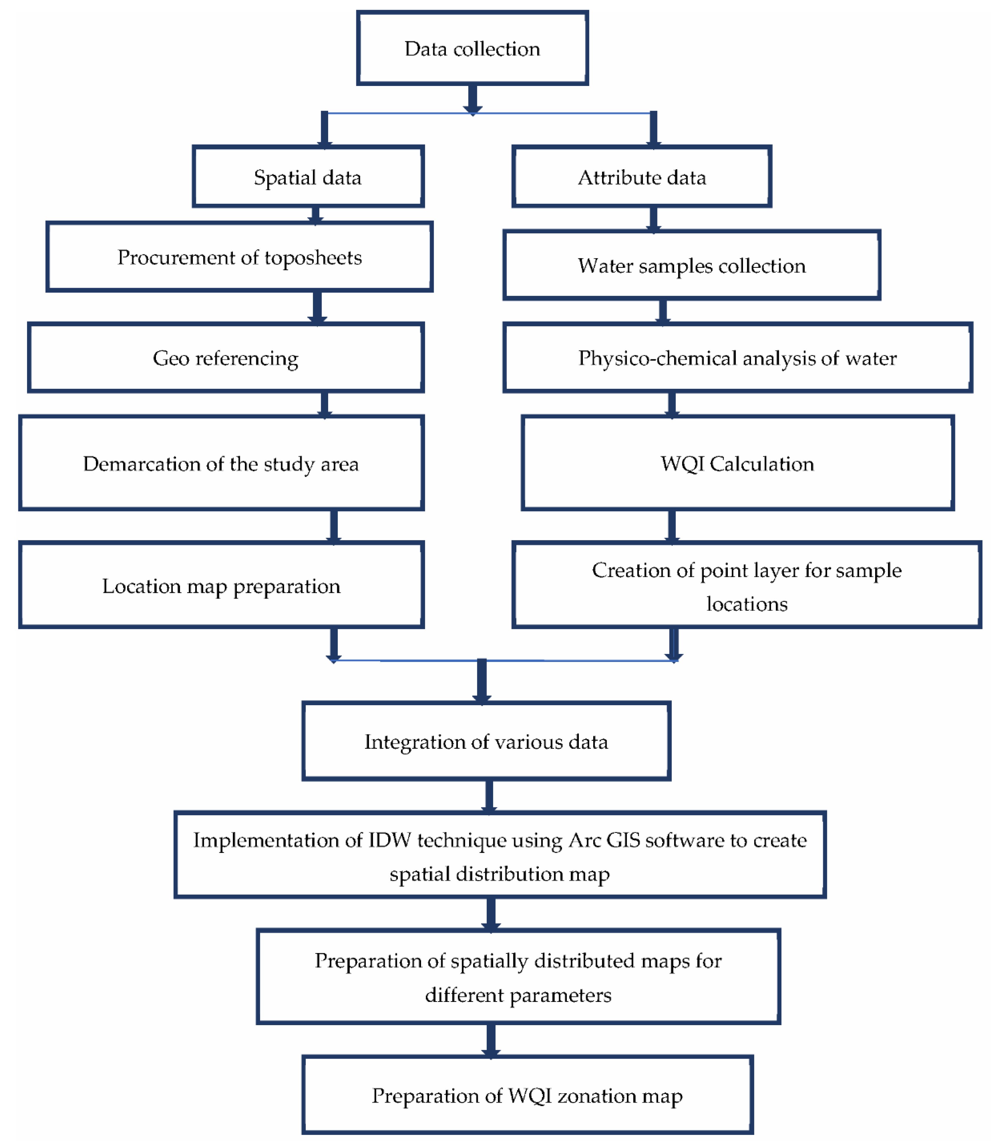
3.1. Data Collection and Water Quality Estimation
3.2. Utilization of AI for the Prediction of the WQI
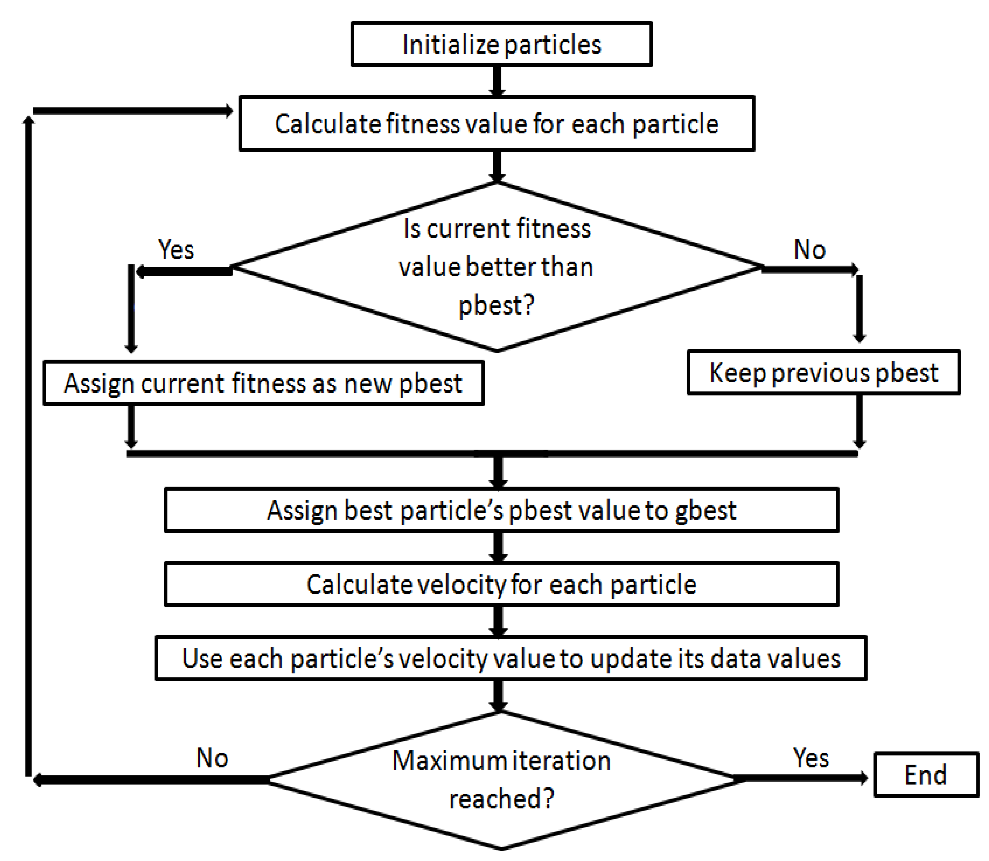
3.2.1. Classification and Prediction Using a PSO–SVM Approach Based on the Water Quality Index
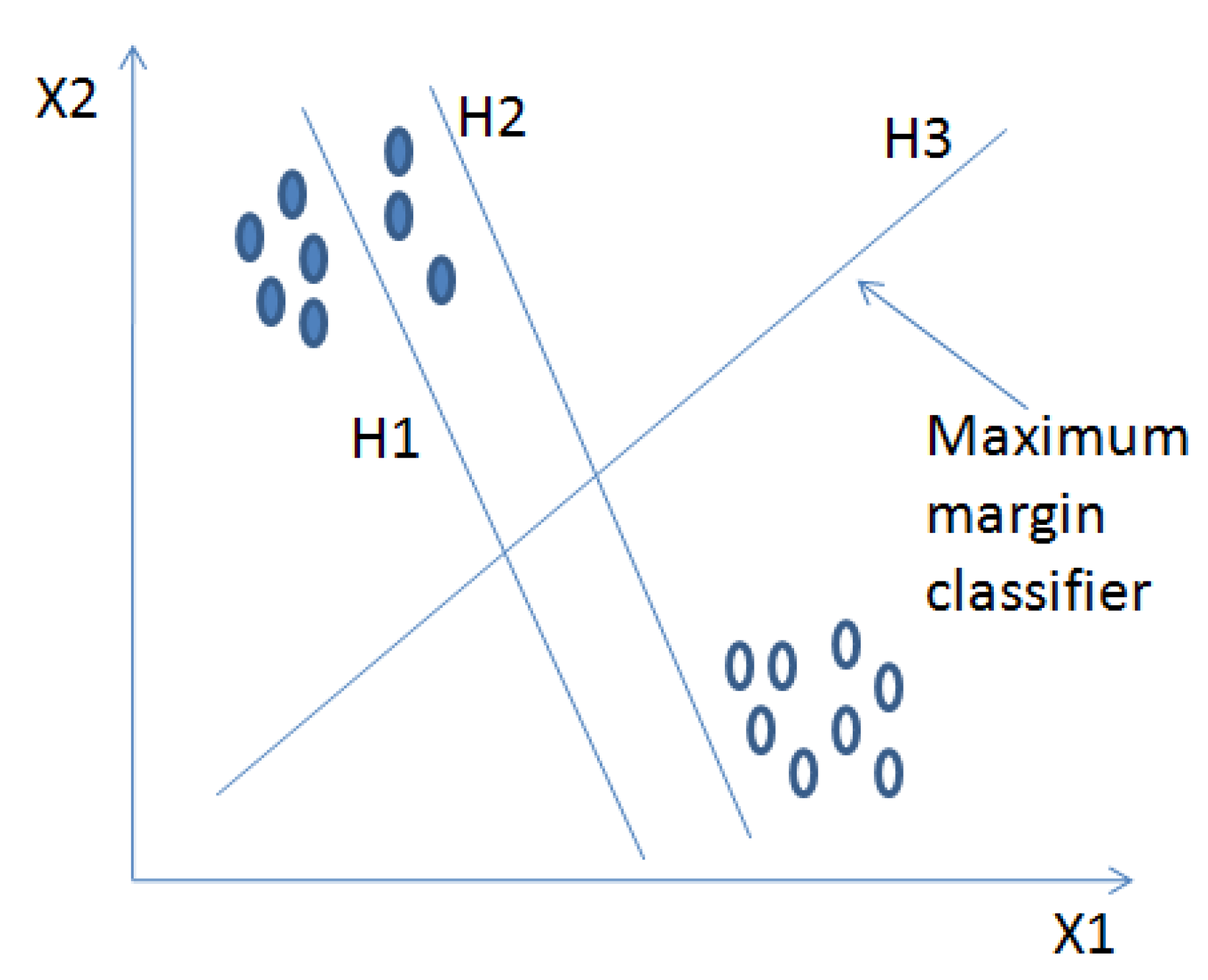
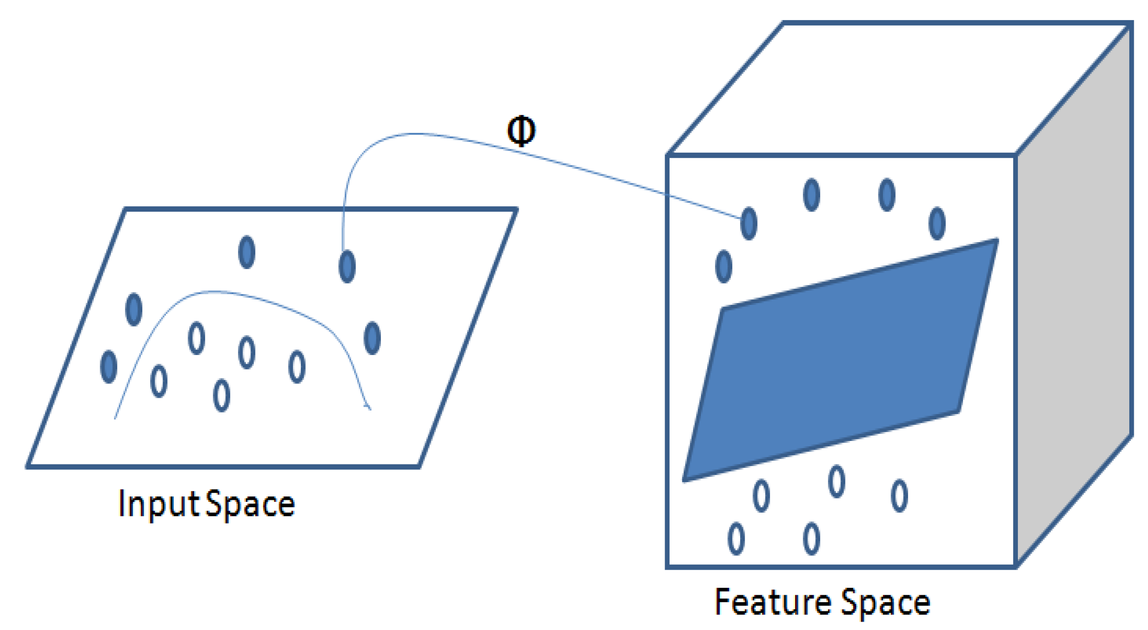
3.2.2. Classification Using a Support Vector Machine
3.2.3. Classification Using Naive Bayes Classifier
4. Results and Discussion
4.1. Water Quality Index (WQI) Analysis of the Field-Based Samples
4.2. Result from the PSO–SVM Study
4.3. Discussion of the PSO–NBC Approach
4.4. Comparison between the PSO–SVM and PSO–NBC Approaches
5. Conclusions
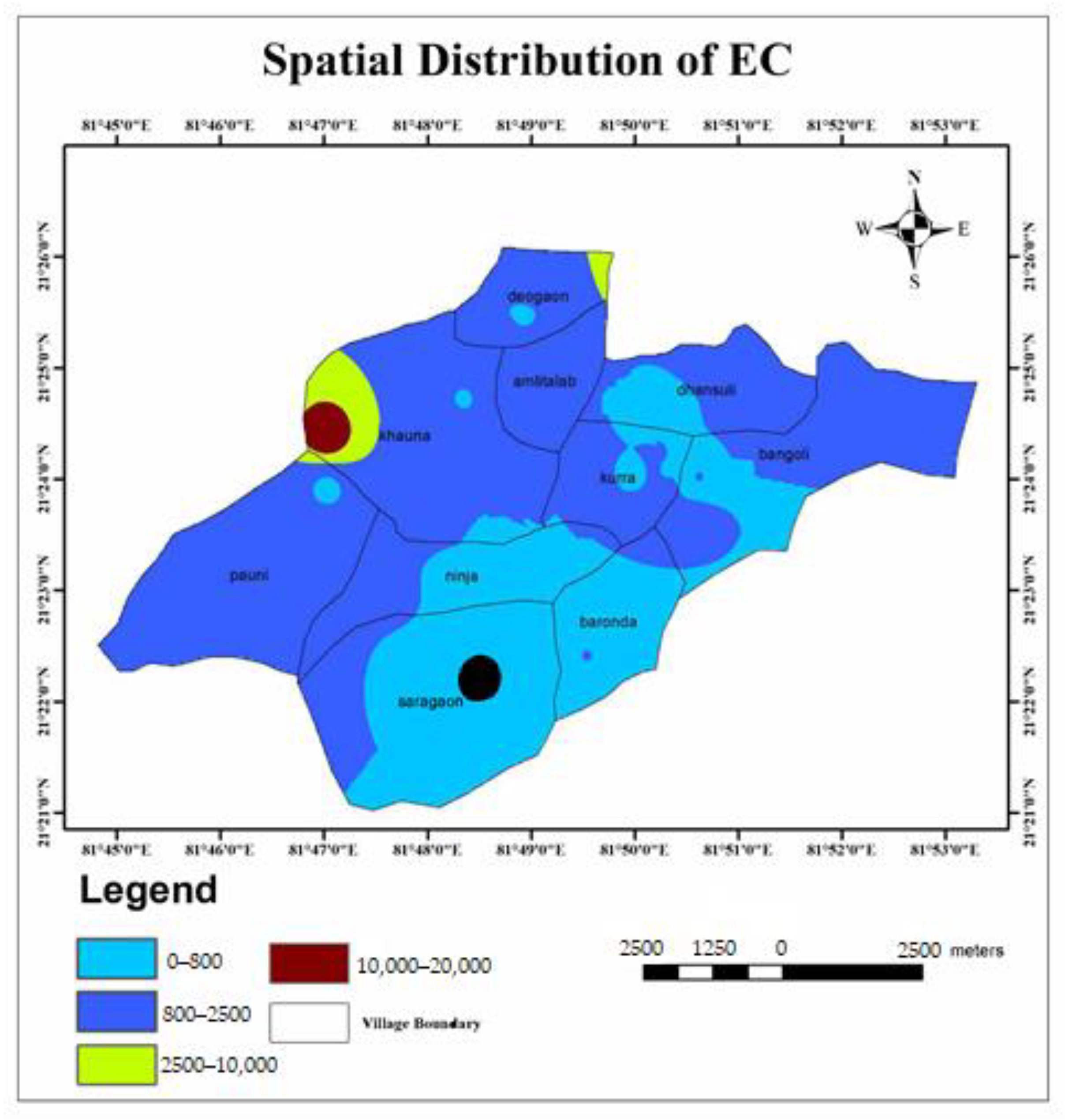
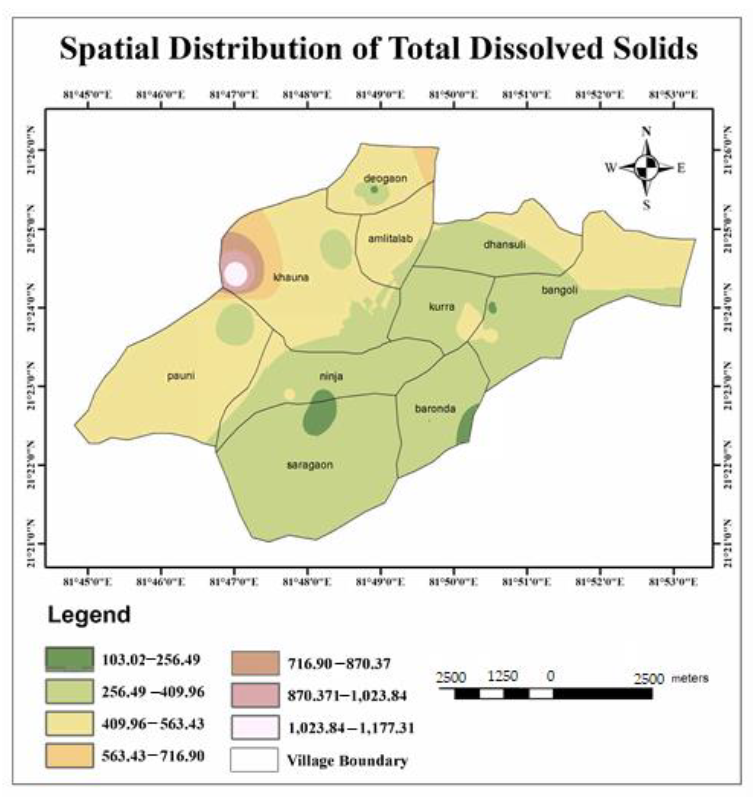
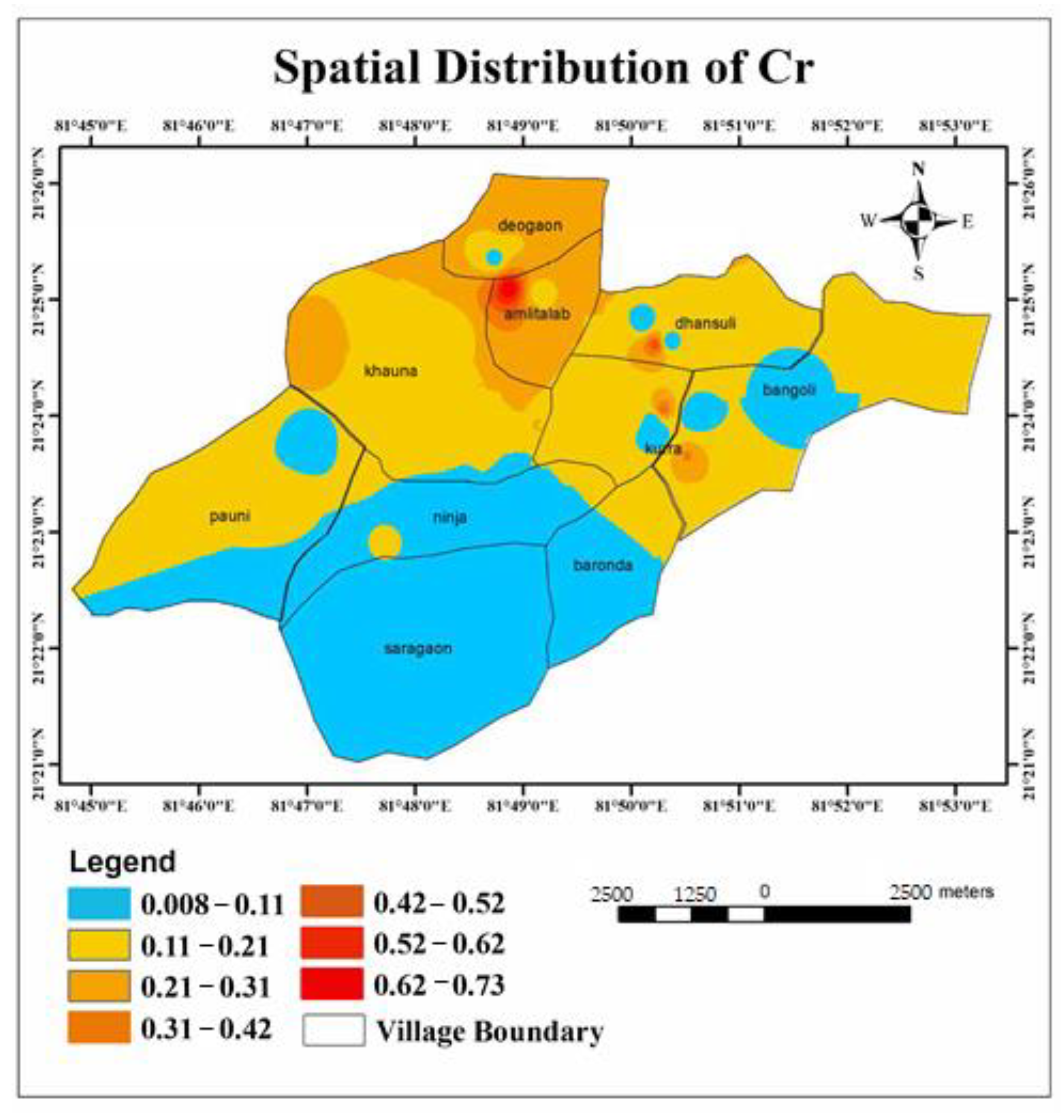
- The calculated WQI values suggested that 32.43% and 43.24% of the water samples of the study area represented excellent and good water qualities, respectively. Similarly, it can also be observed that 21.62% and 2.71% of the water in the study area were of poor and very poor drinking water qualities. Very poor water quality was observed from the Raikheda pond area due to very high chromium concentration. Poor water quality was observed in significant parts of the Deogaon, Dhansuli, Bangoli, Amlitalab, and Khauna villages.
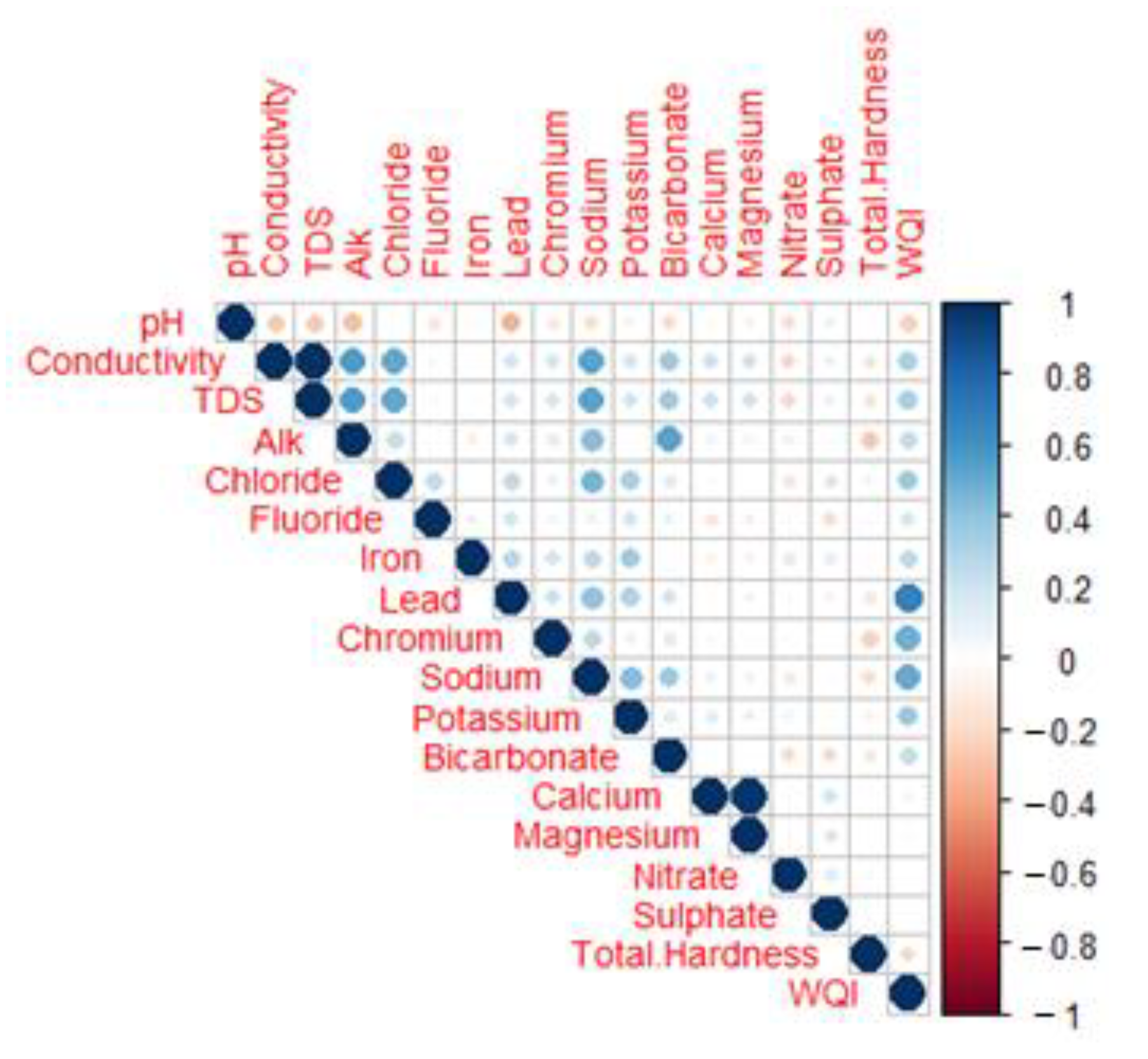
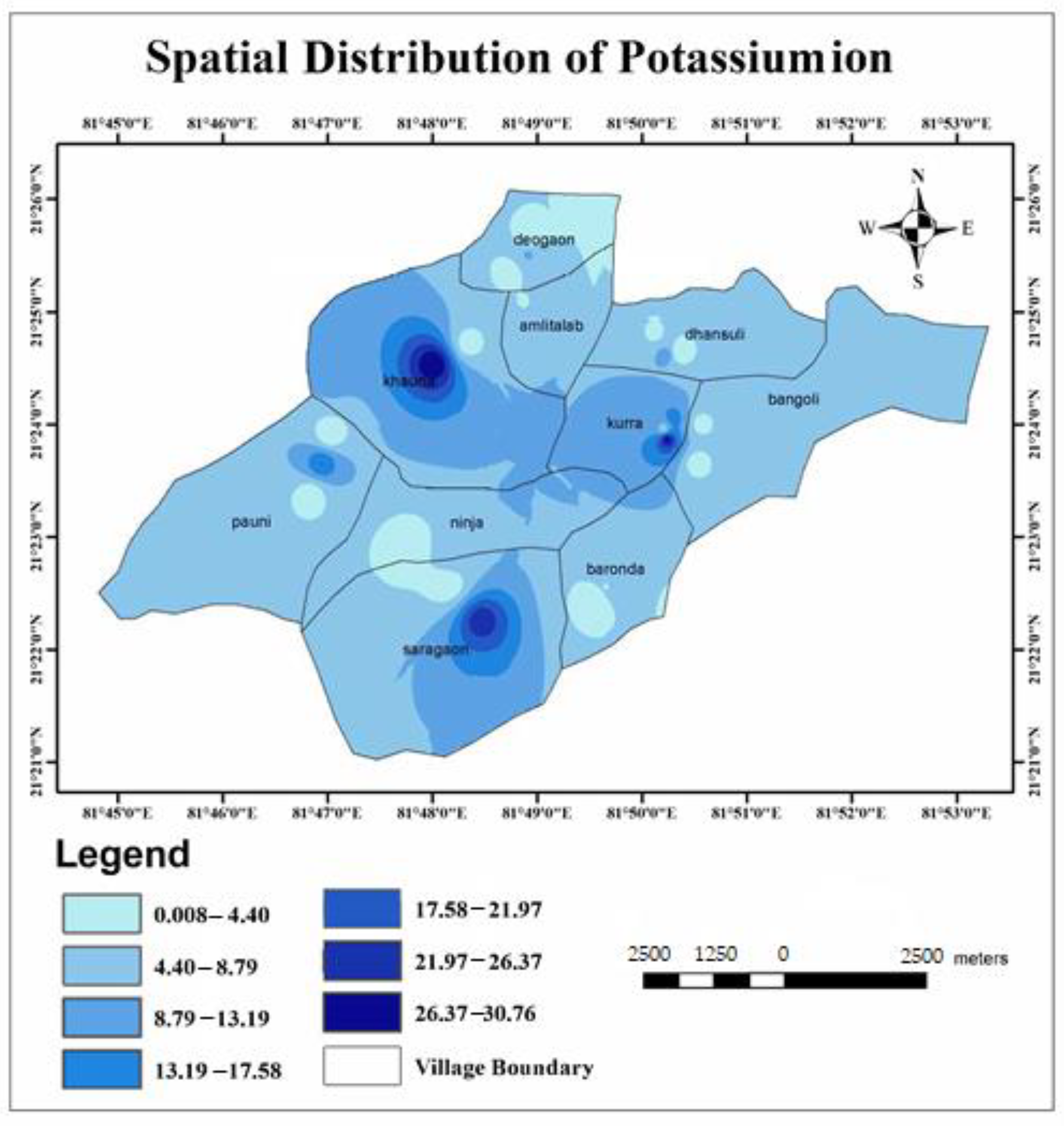
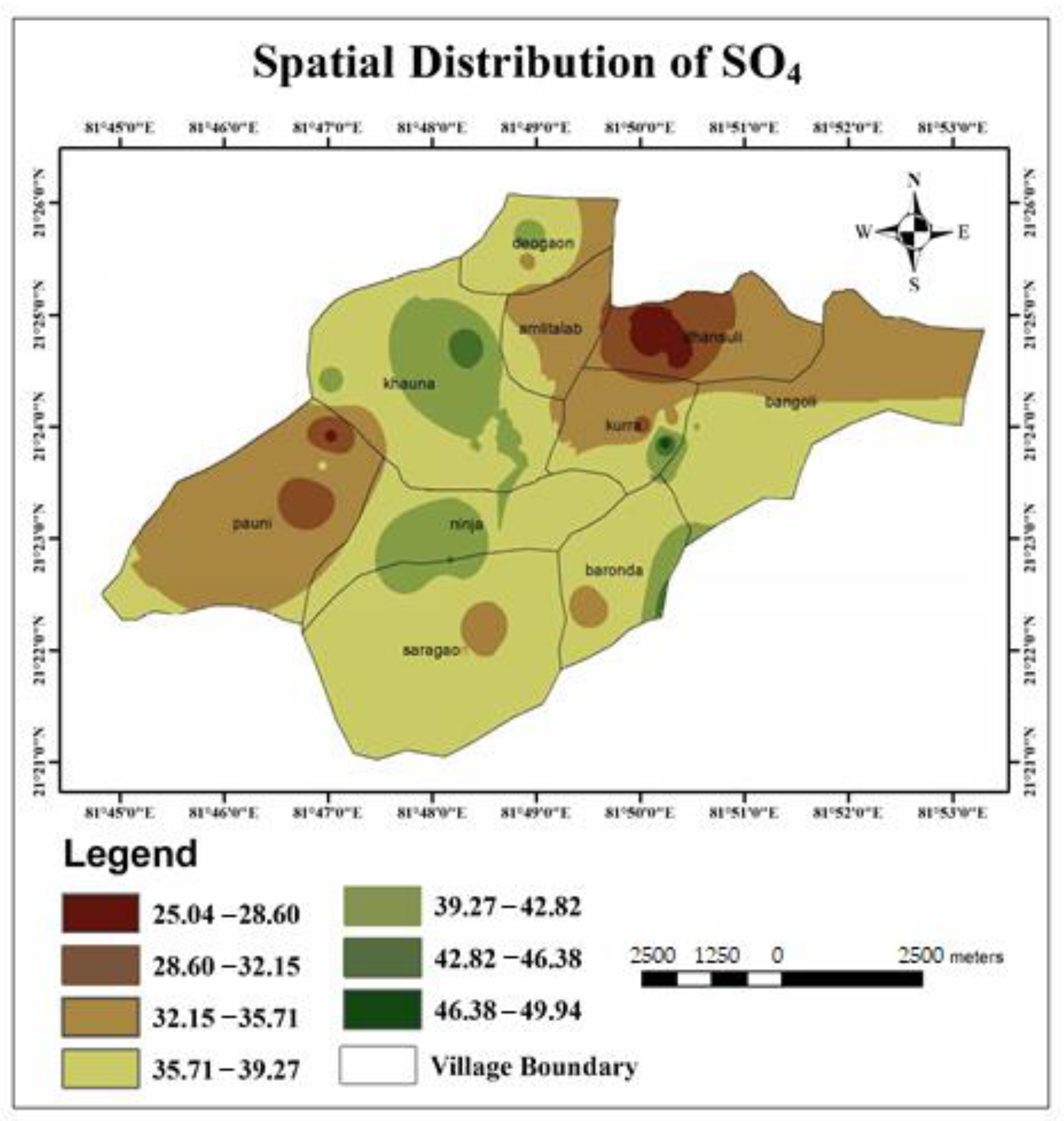
- The major cation and anion data revealed that all anions were within the limits, except for potassium, where 13% of the samples exceeded the limit. However, the heavy metals pollution in the area due to mining activities could be a cause for concern soon. A total of 48.6% of the samples from the area exceeded the permissible limits of chromium, which can cause conditions such as hearing loss, blood disorders, hypertension, and death at high levels.
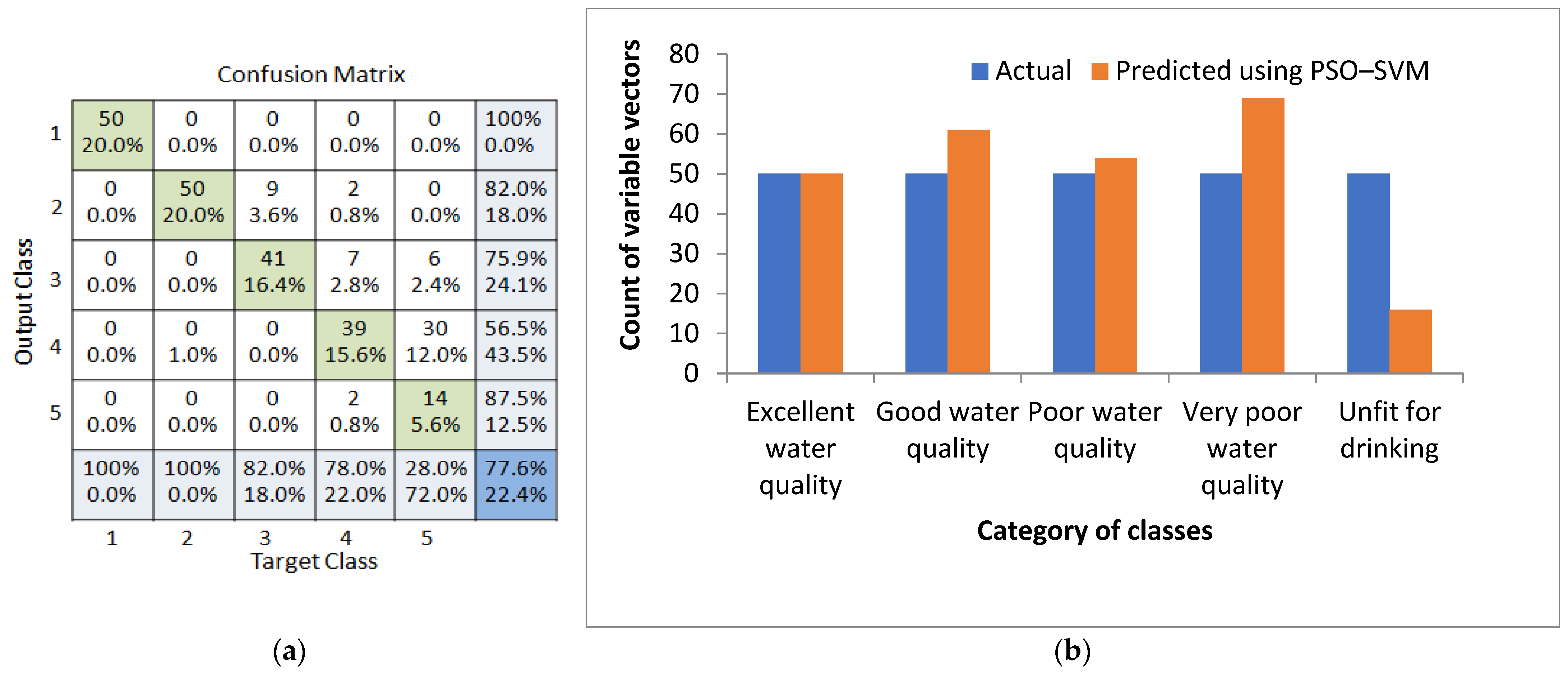
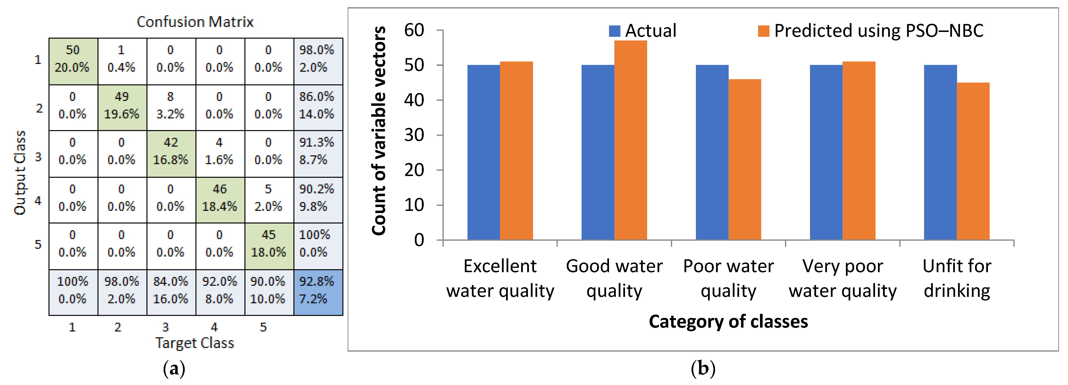
- The study further suggests that ensemble machine learning algorithms can be used for the estimation and prediction of a WQI with significant accuracies. In the present study, a particle swarm optimization approach coupled with a naive Bayes classifier provided a 92.8% accurate prediction of the WQI indices. Therefore, with the help of a user interface, this algorithm can be efficiently utilized for the estimation of WQIs, which can save significant effort and time.
Author Contributions
Funding
Institutional Review Board Statement
Informed Consent Statement
Data Availability Statement
Acknowledgments
Conflicts of Interest
Appendix A

| Sample No. | Lat | Long | Sample No. | Lat | Long | Sample No. | Lat | Long |
|---|---|---|---|---|---|---|---|---|
| 1 | 81.8282 | 21.3761 | 13 | 81.8367 | 21.3994 | 25 | 81.8155 | 21.4273 |
| 2 | 81.8023 | 21.3764 | 14 | 81.8373 | 21.3977 | 26 | 81.8124 | 21.4226 |
| 3 | 81.8077 | 21.371 | 15 | 81.834 | 21.4001 | 27 | 81.8152 | 21.4252 |
| 4 | 81.7961 | 21.3815 | 16 | 81.828 | 21.3760 | 28 | 81.8584 | 21.4041 |
| 5 | 81.8028 | 21.3801 | 17 | 81.8258 | 21.3736 | 29 | 81.8377 | 21.4311 |
| 6 | 81.7961 | 21.3815 | 18 | 81.8282 | 21.3761 | 30 | 81.8566 | 21.4033 |
| 7 | 81.8391 | 21.4107 | 19 | 81.7824 | 21.3942 | 31 | 81.8001 | 21.4089 |
| 8 | 81.8353 | 21.4134 | 20 | 81.7807 | 21.3896 | 32 | 81.8426 | 21.4000 |
| 9 | 81.8371 | 21.4103 | 21 | 81.7837 | 21.3985 | 33 | 81.8405 | 21.3729 |
| 10 | 81.8383 | 21.4010 | 22 | 81.7837 | 21.4066 | 34 | 81.8384 | 21.4329 |
| 11 | 81.842 | 21.3943 | 23 | 81.8001 | 21.4089 | 35 | 81.8384 | 21.4325 |
| 12 | 81.8433 | 21.4002 | 24 | 81.8056 | 21.4119 | 36 | 81.819 | 21.4177 |
| 37 | 81.8145 | 21.4183 |


References
- Islam, S.; Rasul, T.; Bin Alam, J.; Haque, M.A. Evaluation of Water Quality of the Titas River Using NSF Water Quality Index. J. Sci. Res. 2010, 3, 151. [Google Scholar] [CrossRef]
- Al-Zahrani, M.A.; Abo-Monasar, A. Urban Residential Water Demand Prediction Based on Artificial Neural Networks and Time Series Models. Water Resour. Manag. 2015, 29, 3651–3662. [Google Scholar] [CrossRef]
- Elkiran, G.; Ergil, M. The assessment of a water budget of North Cyprus. Build. Environ. 2006, 41, 1671–1677. [Google Scholar] [CrossRef]
- Shalby, A.; Elshemy, M.; Zeidan, B.A. Assessment of Climate Change Impacts on Water Quality Parameters of Lake Burullus, Egypt. Environ. Sci. Poll. Res. 2019, 27, 1–22. [Google Scholar] [CrossRef] [PubMed]
- Kavitha, R.; Elangovan, K. Ground water quality characteristics at Erode district, Tamilnadu India. Int. J. Environ. Sci. 2010, 1, 163–175. [Google Scholar]
- Sharma, D.; Kansal, A. Water quality analysis of River Yamuna using water quality index in the national capital territory, India (2000–2009). Appl. Water Sci. 2011, 1, 147–157. [Google Scholar] [CrossRef]
- Smith, D.G. A better water quality indexing system for rivers and streams. Water Res. 1990, 24, 1237–1244. [Google Scholar] [CrossRef]
- Kannel, P.R.; Lee, S.; Lee, Y.-S.; Kanel, S.R.; Khan, S.P. Application of Water Quality Indices and Dissolved Oxygen as Indicators for River Water Classification and Urban Impact Assessment. Environ. Monit. Assess. 2007, 132, 93–110. [Google Scholar] [CrossRef]
- Singh, R.P.; Nath, S.; Prasad, S.C.; Nema, A.K. Selection of Suitable Aggregation Function for Estimation of Aggregate Pollution Index for River Ganges in India. J. Environ. Eng. 2008, 134, 689–701. [Google Scholar] [CrossRef]
- Yadav, N.S.; Kumar, A.; Sharma, M. Ecological health assessment of Chambal River using water quality parameters. J. Integr. Sci. Technol. 2014, 2, 52–56. [Google Scholar]
- Agrawal, P.; Sinha, A.; Pasupuleti, S.; Nune, R.; Saha, S. Geospatial Analysis Coupled with Logarithmic Method for Water Quality Assessment in Part of Pindrawan Tank Command Area in Raipur District of Chhattisgarh. In Climate Impacts on Water Resources in India; Springer: Berlin, Germany, 2021; pp. 57–78. [Google Scholar]
- Hameed, M.; Sharqi, S.S.; Yaseen, Z.M.; Afan, H.A.; Hussain, A.; Elshafie, A. Application of artificial intelligence (AI) techniques in water quality index prediction: A case study in tropical region, Malaysia. Neural Comput. Appl. 2017, 28, 893–905. [Google Scholar] [CrossRef]
- Rufino, F.; Busico, G.; Cuoco, E.; Darrah, T.H.; Tedesco, D. Evaluating the Suitability of Urban Groundwater Resources for Drinking Water and Irrigation Purposes: An Integrated Approach in the Agro-Aversano Area of Southern Italy. Environ. Monit. Assess. 2019, 191, 1–17. [Google Scholar] [CrossRef] [PubMed]
- Vadiati, M.; Asghari-Moghaddam, A.; Nakhaei, M.; Adamowski, J.; Akbarzadeh, A. A fuzzy-logic based decision-making approach for identification of groundwater quality based on groundwater quality indices. J. Environ. Manag. 2016, 184, 255–270. [Google Scholar] [CrossRef] [PubMed]
- Bournaris, T.; Papathanasiou, J.; Manos, B.; Kazakis, N.; Voudouris, K. Support of irrigation water use and eco-friendly decision process in agricultural production planning. Oper. Res. 2015, 15, 289–306. [Google Scholar] [CrossRef]
- Sargaonkar, A.; Deshpande, V. Development of an Overall Index of Pollution for Surface Water Based on a General Classification Scheme in Indian Context. Environ. Monit. Assess. 2003, 89, 43–67. [Google Scholar] [CrossRef]
- Gazzaz, N.M.; Yusoff, M.K.; Aris, A.Z.; Juahir, H.; Ramli, M.F. Artificial neural network modeling of the water quality index for Kinta River (Malaysia) using water quality variables as predictors. Mar. Pollut. Bull. 2012, 64, 2409–2420. [Google Scholar] [CrossRef]
- Leong, W.C.; Bahadori, A.; Zhang, J.; Ahmad, Z. Prediction of water quality index (WQI) using support vector machine (SVM) and least square-support vector machine (LS-SVM). Int. J. River Basin Manag. 2019, 1–8. [Google Scholar] [CrossRef]
- Iticescu, C.; Georgescu, L.P.; Murariu, G.; Topa, C.; Timofti, M.; Pintilie, V.; Arseni, M.; Timofti, M. Lower Danube Water Quality Quantified through WQI and Multivariate Analysis. Water 2019, 11, 1305. [Google Scholar] [CrossRef]
- Yaseen, Z.M.; Ramal, M.M.; Diop, L.; Jaafar, O.; Demir, V.; Kisi, O. Hybrid adaptive neuro-fuzzu models for water quality index estimation. Water Resour. Manag. 2018, 32, 2227–2245. [Google Scholar] [CrossRef]
- Diamantopoulou, M.J.; Papamichail, D.M.; Antonopoulos, V.Z. The use of a Neural Network technique for the prediction of water quality parameters. Oper. Res. 2005, 5, 115–125. [Google Scholar] [CrossRef]
- Khalil, B.; Ouarda, T.; St-Hilaire, A. Estimation of water quality characteristics at ungauged sites using artificial neural networks and canonical correlation analysis. J. Hydrol. 2011, 405, 277–287. [Google Scholar] [CrossRef]
- Gupta, R.; Singh, A.N.; Singhal, A. Application of ANN for Water Quality Index. Int. J. Mach. Learn. Comput. 2019, 9, 688–693. [Google Scholar] [CrossRef]
- Isiyaka, H.A.; Mustapha, A.; Juahir, H.; Phil-Eze, P. Water quality modelling using artificial neural network and multivariate statistical techniques. Model. Earth Syst. Environ. 2019, 5, 583–593. [Google Scholar] [CrossRef]
- Nourani, V.; Elkiran, G.; Abdullahi, J. Multi-station artificial intelligence based ensemble modeling of reference evapotranspiration using pan evaporation measurements. J. Hydrol. 2019, 577, 123958. [Google Scholar] [CrossRef]
- Gaya, M.S.; Abba, S.I.; Abdu, A.M.; Tukur, A.I.; Saleh, M.A.; Esmaili, P.; Wahab, N.A. Estimation of Water Quality Index Using Artificial Intelligence Approaches and Multi-Linear Regression. Int. J. Artif. Intell. ISSN 2020, 2252, 8938. [Google Scholar] [CrossRef]
- Najah, A.; El-Shafie, A.H.; Karim, O.A. Performance of ANFIS versus MLP-NN dissolved oxygen prediction models in water quality monitoring. Environ. Sci. Pollut. Res. 2014, 21, 1658–1670. [Google Scholar] [CrossRef] [PubMed]
- Ahmed, A.N.; Othman, F.B.; Afan, H.A.; Ibrahim, R.K.; Fai, C.M.; Hossain, S.; Ehteram, M.; Elshafie, A. Machine learning methods for better water quality prediction. J. Hydrol. 2019, 578, 124084. [Google Scholar] [CrossRef]
- Karim, S.A.A.; Kamsani, N.F. Water Quality Index Using Fuzzy Regression. In Water Quality Index Prediction Using Multiple Linear Fuzzy Regression Model; Springer: New York, NY, USA, 2020; pp. 37–53. [Google Scholar]
- Nayak, J.G.; Patil, L.; Patki, V.K. Development of water quality index for Godavari River (India) based on fuzzy inference system. Groundw. Sustain. Dev. 2020, 10, 100350. [Google Scholar] [CrossRef]
- Yasin, M.I.; Karim, S.A.A. A New Fuzzy Weighted Multivariate Regression to Predict Water Quality Index at Perak Rivers. In Optimization Based Model Using Fuzzy and Other Statistical Techniques towards Environmental Sustainability; Springer: New York, NY, USA, 2020; pp. 1–27. [Google Scholar]
- Abobakr Yahya, A.S.; Ahmed, A.N.; Binti Othman, F.; Ibrahim, R.K.; Afan, H.A.; El-Shafie, A.; Fai, C.M.; Hossain, M.S.; Ehteram, M.; Elshafie, A. Water Quality Prediction Model Based Support Vector Machine Model for Ungauged River Catchment under Dual Scenarios. Water 2019, 11, 1231. [Google Scholar] [CrossRef]
- Abba, S.I.; Pham, Q.B.; Saini, G.; Linh, N.T.T.; Ahmed, A.N.; Mohajane, M.; Khaledian, M.; Abdulkadir, R.A.; Bach, Q.-V. Implementation of data intelligence models coupled with ensemble machine learning for prediction of water quality index. Environ. Sci. Pollut. Res. 2020, 27, 41524–41539. [Google Scholar] [CrossRef]
- Elkiran, G.; Nourani, V.; Abba, S. Multi-step ahead modelling of river water quality parameters using ensemble artificial intelligence-based approach. J. Hydrol. 2019, 577, 123962. [Google Scholar] [CrossRef]
- BIS (Bureau of Indian Standard). Indian Standard Drinking Water–Specification; Second Revision; Bureau of Indian Standards (BIS): New Delhi, India, 2012. [Google Scholar]
- Chaurasia, A.K.; Pandey, H.K.; Tiwari, S.K.; Prakash, R.; Pandey, P.; Ram, A. Groundwater Quality assessment using Water Quality Index (WQI) in parts of Varanasi District, Uttar Pradesh, India. J. Geol. Soc. India 2018, 92, 76–82. [Google Scholar] [CrossRef]
- WHO. Guidelines for Drinking Water, Recommendations; World Health Organization (WHO): Geneva, Switzerland, 2012. [Google Scholar]
- Yisa, J.; Jimoh, T. Analytical studies on water quality index of river Landzu. Am. J. Appl. Sci. 2010, 7, 453. [Google Scholar] [CrossRef]
- Tyagi, S.; Singh, P.; Sharma, B.; Singh, R. Assessment of Water Quality for Drinking Purpose in District Pauri of Uttarakhand, India. Appl. Ecol. Environ. Sci. 2014, 2, 94–99. [Google Scholar] [CrossRef]
- Akter, T.; Jhohura, F.T.; Akter, F.; Chowdhury, T.R.; Mistry, S.K.; Dey, D.; Barua, M.K.; Islam, A.; Rahman, M. Water Quality Index for measuring drinking water quality in rural Bangladesh: A cross-sectional study. J. Health Popul. Nutr. 2016, 35, 1–12. [Google Scholar] [CrossRef]
- Ramakrishnaiah, C.R.; Sadashivaiah, C.; Ranganna, G. Assessment of Water Quality Index for the Groundwater in Tumkur Taluk, Karnataka State, India. E-J. Chem. 2009, 6, 523–530. [Google Scholar] [CrossRef]
- Eberhart, R.; Kennedy, J. A New Optimizer Using Particle Swarm Theory; IEEE: Piscataway, NJ, USA, 1995; pp. 39–43. [Google Scholar]
- Gilani, S.-O.; Sattarvand, J.; Hajihassani, M.; Abdullah, S.S. A stochastic particle swarm based model for long term production planning of open pit mines considering the geological uncertainty. Resour. Policy 2020, 68, 101738. [Google Scholar] [CrossRef]
- Yasin, Q.; Sohail, G.M.; Ding, Y.; Ismail, A.; Du, Q. Estimation of Petrophysical Parameters from Seismic Inversion by Combining Particle Swarm Optimization and Multilayer Linear Calculator. Nat. Resour. Res. 2020, 29, 3291–3317. [Google Scholar] [CrossRef]
- Mehrabi, M.; Pradhan, B.; Moayedi, H.; Alamri, A. Optimizing an Adaptive Neuro-Fuzzy Inference System for Spatial Prediction of Landslide Susceptibility Using Four State-of-the-art Metaheuristic Techniques. Sensors 2020, 20, 1723. [Google Scholar] [CrossRef] [PubMed]
- Sun, D.; Wen, H.; Wang, D.; Xu, J. A random forest model of landslide susceptibility mapping based on hyperparameter optimization using Bayes algorithm. Geomorphol. 2020, 362, 107201. [Google Scholar] [CrossRef]
- Gafar, A.A.; Khayat, M.E.; Ahmad, S.A.; Yasid, N.A.; Shukor, M.Y. Response Surface Methodology for the Optimization of Keratinase Production in Culture Medium Containing Feathers by Bacillus sp. UPM-AAG1. Catalysts 2020, 10, 848. [Google Scholar] [CrossRef]
- Bui, Q.-T.; Nguyen, Q.-H.; Nguyen, X.L.; Pham, V.D.; Nguyen, H.D.; Pham, V.-M. Verification of novel integrations of swarm intelligence algorithms into deep learning neural network for flood susceptibility mapping. J. Hydrol. 2020, 581, 124379. [Google Scholar] [CrossRef]
- Pourghasemi, H.R.; Razavi-Termeh, S.V.; Kariminejad, N.; Hong, H.; Chen, W. An assessment of metaheuristic approaches for flood assessment. J. Hydrol. 2020, 582, 124536. [Google Scholar] [CrossRef]
- Roshanravan, B.; Aghajani, H.; Yousefi, M.; Kreuzer, O. Particle Swarm Optimization Algorithm for Neuro-Fuzzy Prospectivity Analysis Using Continuously Weighted Spatial Exploration Data. Nat. Resour. Res. 2018, 28, 309–325. [Google Scholar] [CrossRef]
- Engelbrecht, A.P. Computational Intelligence: An Introduction, 2nd ed.; Jonh Wiley & Sons, Ltd.: Chichester, UK, 2007; Volume 1. [Google Scholar]
- Clerc, M.; Kennedy, J. The particle swarm—Explosion, stability, and convergence in a multidimensional complex space. IEEE Trans. Evol. Comput. 2002, 6, 58–73. [Google Scholar] [CrossRef]
- Ciarelli, P.M.; Krohling, R.A.; Oliveira, E. Particle swarm optimization applied to parameters learning of probabilistic neural networks for classification of economic activities. In Particle Swarm Optimization; InTech: Rijeka, Croatia, 2009; pp. 313–327. [Google Scholar]
- Scholkopf, B.; Sung, K.-K.; Burges, C.J.C.; Girosi, F.; Niyogi, P.; Poggio, T.; Vapnik, V. Comparing support vector machines with Gaussian kernels to radial basis function classifiers. IEEE Trans. Signal Process. 1997, 45, 2758–2765. [Google Scholar] [CrossRef]
- Dibike, Y.B.; Velickov, S.; Solomatine, D.; Abbott, M.B. Model Induction with Support Vector Machines: Introduction and Applications. J. Comput. Civ. Eng. 2001, 15, 208–216. [Google Scholar] [CrossRef]
- Li, C.-H.; Lin, C.-T.; Kuo, B.-C.; Ho, H.-H. An Automatic Method for Selecting the Parameter of the Normalized Kernel Function to Support Vector Machines. In Proceedings of the 2010 International Conference on Technologies and Applications of Artificial Intelligence, Hsinchu, Taiwan, 18–20 November 2010; pp. 226–232. [Google Scholar]
- Shukla, R.; Chakraborty, A.; Sachdeva, K.; Joshi, P.K. Agriculture in the western Himalayas—An asset turning into a liability. Dev. Pract. 2017, 28, 318–324. [Google Scholar] [CrossRef]
- Shukla, R.; Sachdeva, K.; Joshi, P.K. Demystifying vulnerability assessment of agriculture communities in the Himalayas: A systematic review. Nat. Hazards 2017, 91, 409–429. [Google Scholar] [CrossRef]


| Parameters | Indian Standards | Weight (Wi) | Unit Weight (Wi) | Parameters | Indian Standards | Weight (Wi) | Unit Weight (Wi) |
|---|---|---|---|---|---|---|---|
| EC | 300 | 1 | 0.024 | Alkalinity | 200 | 3 | 0.073 |
| PH | 6.5−8.5 | 2 | 0.049 | TH | 300 | 2 | 0.049 |
| TDS | 500 | 3 | 0.073 | Fluoride | 1 | 4 | 0.098 |
| Calcium | 75 | 2 | 0.049 | Iron | 0.3 | 4 | 0.098 |
| Magnesium | 30 | 2 | 0.049 | Chromium | 0.05 | 4 | 0.073 |
| Potassium | 12 | 2 | 0.049 | Chloride | 250 | 2 | 0.049 |
| Sodium | 200 | 1 | 0.022 | Bicarbonate | 250 | 3 | 0.073 |
| Sulfate | 200 | 3 | 0.073 | Total | 41 | 1 | |
| Nitrate | 45 | 3 | 0.073 |
| WQI | Class |
|---|---|
| 0−50 | Excellent water quality |
| 50−100 | Good water quality |
| 100−200 | Poor water quality |
| 200−300 | Very poor water quality |
| >300 | Unfit for drinking |
| Parameter | Experimentally Obtained Range of Concentration in the Collected Samples | Permissible Limits | Percentage of Samples Exceeding Permissible Limits | Undesirable Effect |
|---|---|---|---|---|
| pH | 7.26–8.59 | 6.5 to 8.5 | 2.70 | Irritation in eyes, skin, and mucous membranes; skin disorders |
| EC | 152–1998 | 300 | 89.19 | Cardiac dysrhythmias |
| TDS (mg/L) | 98.8–1199 | 500 | 21.62 | Gastrointestinal irritation |
| Alkalinity (mg/L) | 60–335 | 200 | 29.73 | Unpleasant and harmful to aquatic life and humans |
| Chloride (mg/L) | 20–330 | 250 | 8.11 | Salty taste |
| Calcium (mg/L) | 4–60.5 | 75 | 0 | Scale formation |
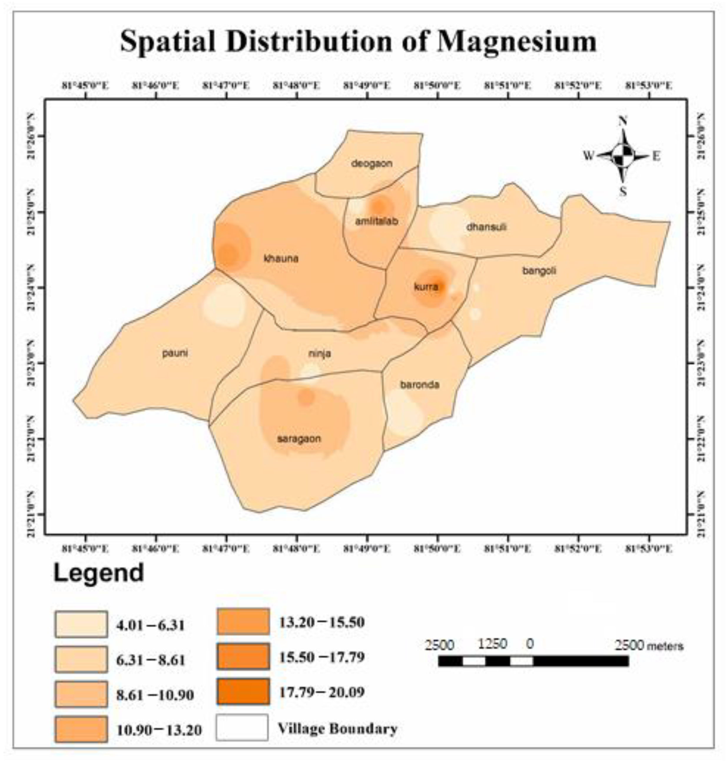
| Magnesium (mg/L) | 4–20.2 | 30 | 0 | Cerebrovascular disease (Yang, 1998) |
| Potassium (mg/L) | 0–30.9 | 12 | 16.20 | Bitter taste |
| Sodium(mg/L) | 1.2–18.3 | 200 | 0 | High blood pressure |
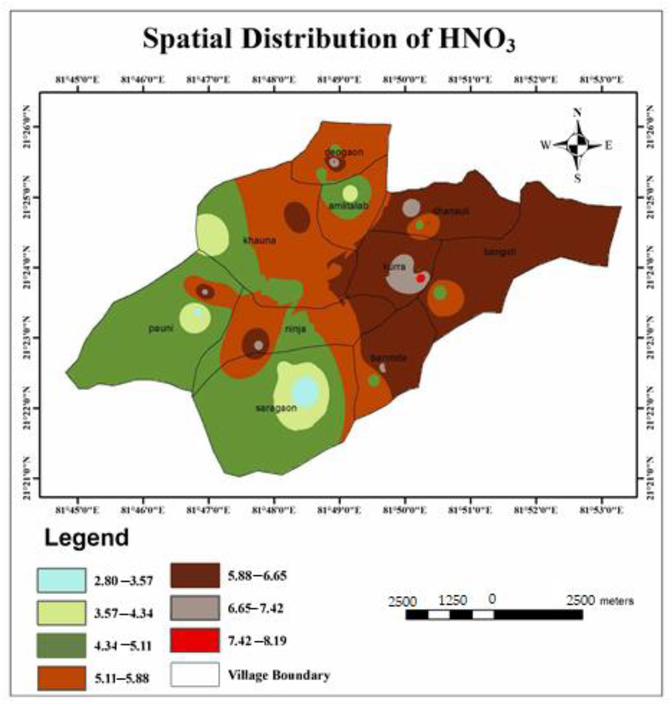
| Nitrate (mg/L) | 3.4–8.2 | 45 | 0 | Methemoglobinemia |
| Sulfate (mg/L) | 25–50 | 200 | 0 | Laxative effect |
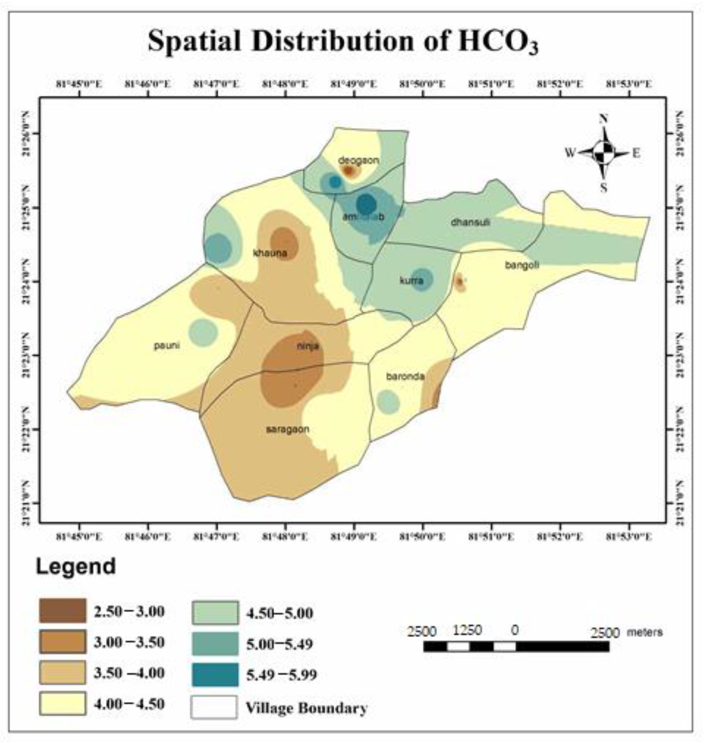
| Bicarbonate (mg/L) | 2.5–6.5 | 250 | 0 | Vomiting, dehydration, chronic obstructive pulmonary disease |
| Fluoride (mg/L) | 0.25–0.84 | 1 | 0 | Mottling of teeth, deformation of bones |
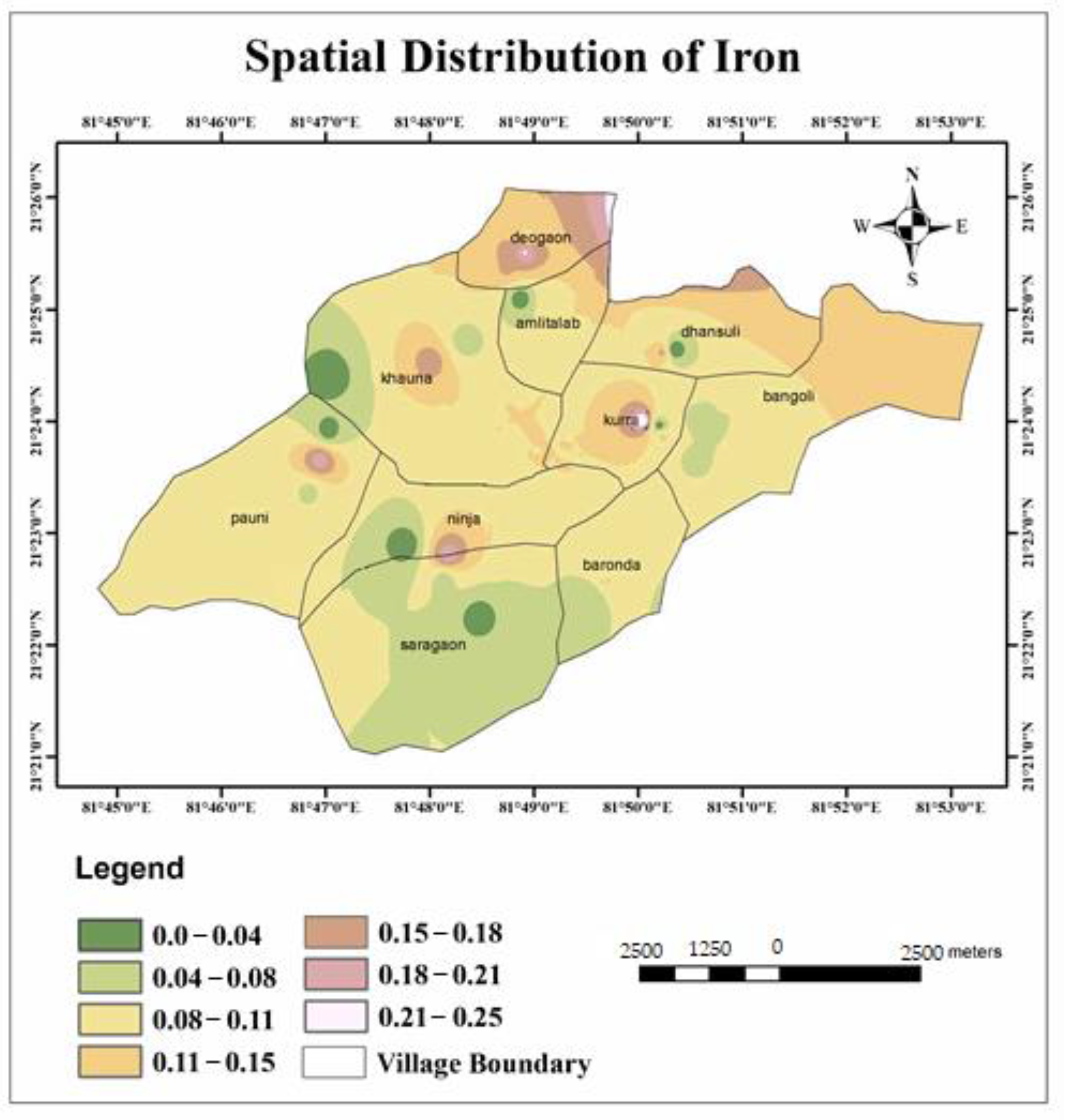
| Iron (mg/L) | 0.015–0.785 | 0.3 | 5.41 | Diabetes, hemochromatosis, stomach problems, nausea, and vomiting |
| Chromium (mg/L) | 0.007–0.737 | 0.05 | 56.76 | Hearing loss, blood disorders, hypertension, death at high levels |
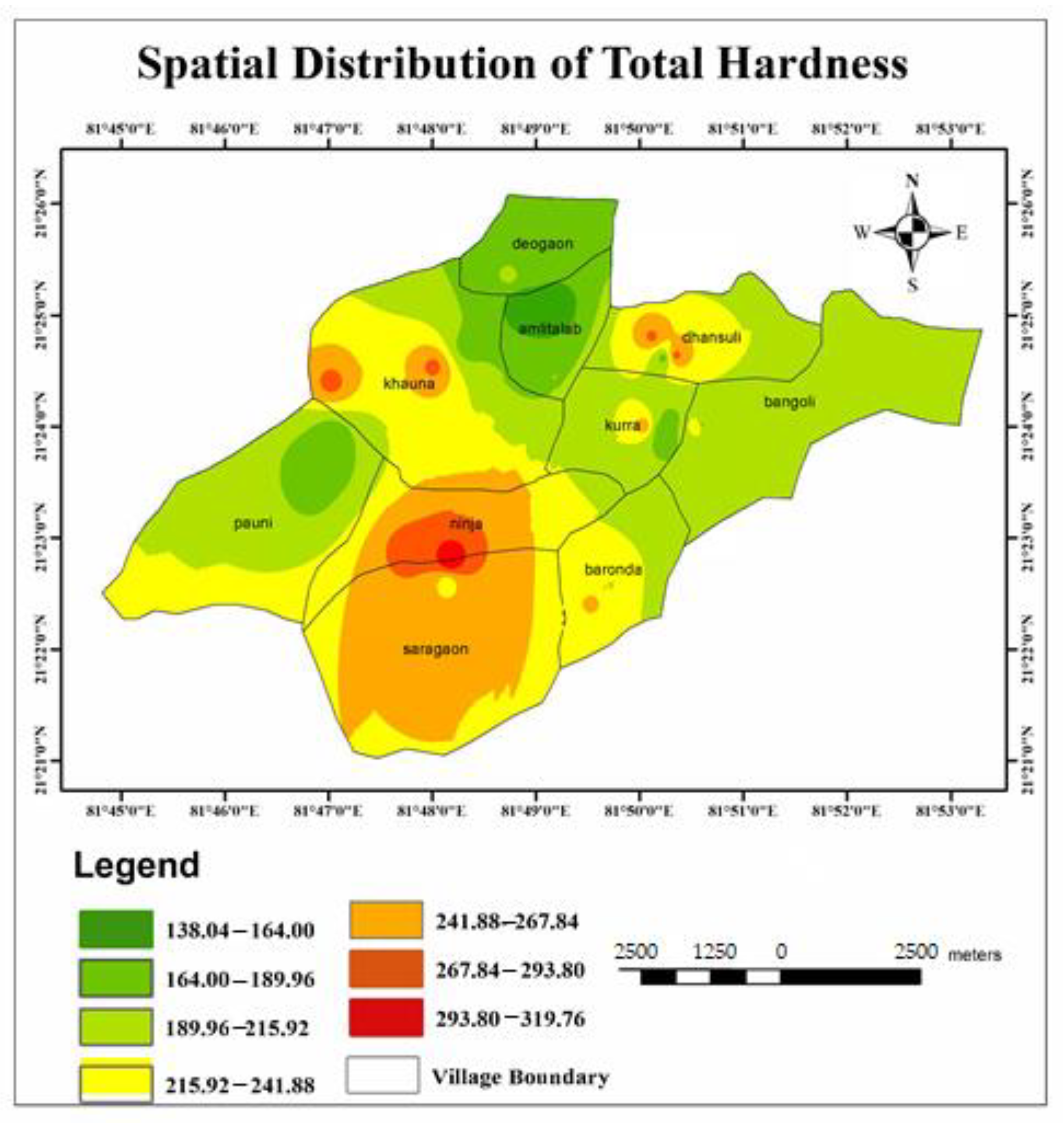
| TH (as mg/L) | 138–320 | 200 | 43.24 | Scale formation in pipes anencephaly, urolithiasis, parental mortality |
Publisher’s Note: MDPI stays neutral with regard to jurisdictional claims in published maps and institutional affiliations. |
© 2021 by the authors. Licensee MDPI, Basel, Switzerland. This article is an open access article distributed under the terms and conditions of the Creative Commons Attribution (CC BY) license (https://creativecommons.org/licenses/by/4.0/).
Share and Cite
Agrawal, P.; Sinha, A.; Kumar, S.; Agarwal, A.; Banerjee, A.; Villuri, V.G.K.; Annavarapu, C.S.R.; Dwivedi, R.; Dera, V.V.R.; Sinha, J.; et al. Exploring Artificial Intelligence Techniques for Groundwater Quality Assessment. Water 2021, 13, 1172. https://doi.org/10.3390/w13091172
Agrawal P, Sinha A, Kumar S, Agarwal A, Banerjee A, Villuri VGK, Annavarapu CSR, Dwivedi R, Dera VVR, Sinha J, et al. Exploring Artificial Intelligence Techniques for Groundwater Quality Assessment. Water. 2021; 13(9):1172. https://doi.org/10.3390/w13091172
Chicago/Turabian StyleAgrawal, Purushottam, Alok Sinha, Satish Kumar, Ankit Agarwal, Ashes Banerjee, Vasanta Govind Kumar Villuri, Chandra Sekhara Rao Annavarapu, Rajesh Dwivedi, Vijaya Vardhan Reddy Dera, Jitendra Sinha, and et al. 2021. "Exploring Artificial Intelligence Techniques for Groundwater Quality Assessment" Water 13, no. 9: 1172. https://doi.org/10.3390/w13091172
APA StyleAgrawal, P., Sinha, A., Kumar, S., Agarwal, A., Banerjee, A., Villuri, V. G. K., Annavarapu, C. S. R., Dwivedi, R., Dera, V. V. R., Sinha, J., & Pasupuleti, S. (2021). Exploring Artificial Intelligence Techniques for Groundwater Quality Assessment. Water, 13(9), 1172. https://doi.org/10.3390/w13091172