Article

Incorporating Stakeholder Knowledge into a Complex Stock Assessment Model: The Case of Eel Recruitment

1
INRAE, UR EABX, 50 avenue de Verdun, CEDEX, 33612 Cestas, France
2
Management of Diadromous Fish in Their Environment, OFB, INRAE, Institut Agro, UNIV PAU & PAYS ADOUR/E2S UPPA, 35042 Rennes, France
3
AZTI, Sustainable Fisheries Management, Txatxarramendi ugartea z/g, 48395 Sukarrieta, Spain
4
CIIMAR, Terminal de Cruzeiros do Porto de Leixões, 4405-208 Matosinhos, Portugal
5
Departamento de Zoología, Universidad de Córdoba, 14080 Córdoba, Spain
6
MARE, Marine and Environmental Sciences Centre, Faculdade de Ciências da Universidade de Lisboa, Campo Grande, 1749-016 Lisbon, Portugal
7
Departamento de Biologia Animal, Faculdade de Ciências da Universidade de Lisboa, Campo Grande, 1749-016 Lisbon, Portugal
8
GRECO, Institute of Aquatic Ecology, University of Girona, 17003 Girona, Spain
9
Office Français de la Biodiversité, 65 rue de St. Brieuc, 35042 Rennes, France
10
IAV, bd de Bretagne, 56130 La Roche Bernard, France
*
Author to whom correspondence should be addressed.
Water 2021, 13(9), 1136; https://doi.org/10.3390/w13091136
Submission received: 23 February 2021 / Revised: 14 April 2021 / Accepted: 16 April 2021 / Published: 21 April 2021

Abstract

:
Mistrust between scientists and non-scientist stakeholders is a key challenge in fishery management. The support of management with complex models is difficult, as these models cannot easily communicate their results to end users, resulting in a lack of confidence. As an example, the complex life cycle of the European eel raises problems of coordination and discussion among the multiple actors involved in the species’ management. The GEREM model has been proposed as a tool for estimating recruitment, but its complexity, which is essential for addressing the characteristics of the species, makes it difficult to understand and accept by all stakeholders. In the context of the SUDOANG project, we proposed a co-parametrisation of this assessment model to tackle this mistrust. Through the use of various questionnaires, stakeholders were involved in two important choices for the model (zone definition and prior construction). Regular workshops and presentations were organised to explain the model rationales and to gather feedback and expectations. The results show that stakeholders have very similar perceptions of the potential definitions of sub-areas of recruitment in south-western Europe, and these perceptions are consistent with the underlying environmental conditions. On the other hand, the stakeholders have contrasting opinions about the exploitation rates of fisheries in different river basins, and the use of their knowledge currently has little effect on GEREM estimates. More importantly, the overall approach of this study is thought to have reconstructed the trust and confidence among participants.

1. Introduction

There is a long history of misunderstandings between scientists and non-scientific actors in fisheries management [1], and rebuilding trust among them is a key challenge [2,3,4]. Fisheries dynamics are hardly predictable [5] and display chaotic behaviour [1,6]. While scientists have developed increasingly complex numerical models and seek general rules to address this issue, uncertainties in the model results, lack of transparency in the assumptions and poor communication regarding how uncertainty is handled throughout the modelling process have fed this mistrust [7]. Recently, participatory approaches have been proposed to address this problem [7,8]. Involving different types of stakeholders in management and assessment procedures appears to represent a valuable solution to share common views on uncertainty [4], increase transparency [7], and benefit from stakeholder knowledge [9,10]. In view of this, the involvement of stakeholders is perceived as an ingredient of the good governance of fisheries [3,7,11].
These questions regarding the mistrust, lack of transparency, uncertainty, and the need for participatory approaches are even more important in the context of the use of complex models to support fisheries management. While complex models have been developed to support fisheries management, their operational use is often limited due to difficulties in communicating the results and the lack of confidence from end users [12]. The European eel (Anguilla anguilla) is an interesting example: its complex and long cycle combined with its large and fragmented distribution area requires the use of complex stock assessment models. The European eel is a catadromous species that reproduces in the Sargasso Sea [13] but spends its growth phase in continental waters from Northern Africa to Norway [14]. After reproduction, larvae are transported by oceanic currents and metamorphose into glass eels when they reach the continental shelf. Then, they penetrate continental waters, progressively become pigmented yellow eels and remain in continental waters throughout their growing stage. After a period of 3 to 20 years, they metamorphose into silver eels and initiate a new migration towards their spawning ground [14]. Despite their large distribution area, the species is panmictic [15] and, as such, should be managed and assessed on a large spatial scale. However, during the growth phase, the stock is partitioned among small-scale scattered waterbodies, in which the eels are subjected to heterogeneous environmental conditions and anthropogenic pressures [16]. In parallel, eels display large diversity in their life history traits, such as the age-at-silvering, the length-at-silvering and the sex ratio, which are correlated to environmental gradients [17,18,19]. As a consequence, eels are often managed and assessed on the regional sub-stock scale, and while there is a need to orchestrate local initiatives over the whole distribution area [20], few models have been proposed to achieve an assessment on such a scale.
The current status of the European eel population urges the improvement of the management of the population. Indeed, its abundance has been dramatically declining since the early 1980s [21,22,23], and the species is considered critically endangered by the IUCN [24]. Though unclear, the causes of this decline probably involved the synergy of various factors of global change, including overexploitation, parasites, contamination, climate change and habitat destruction/fragmentation [25,26]. In this context, the European Council adopted a regulation in 2007, the so-called Eel Regulation (EC) No. 1100/2007. In this regulation, member states were asked to implement Eel Management Plans (EMPs) in their “Eel Management Units” (EMUs, which can be defined as a management area for eels, often corresponding to a river basin district as defined in the Water Framework Directive), enforcing measures to reduce anthropogenic pressures to achieve a minimum of 40% of the escapement that would have occurred in the absence of anthropogenic impacts. However, the lack of coordination among national or regional management scales impairs the overall coherence of these initiatives and threatens the achievement of the objectives [20].
In this context, the SUDOANG project (Interreg Sudoe) aimed to enhance coordination in the management of European eel in south-western Europe by improving the dialogue among stakeholders and providing common standardised assessment tools to managers. Among other actions, two tools were applied in the project. The model, called EDA (Eel Density Analysis) [27], estimates the abundances of yellow and silver eels in river networks. These estimates can subsequently be used to estimate the escapement, one of the indicators that member states should assess as a response to the Eel Regulation, and the mortality by hydropower plants. The second model is called GEREM [28] and assesses the abundance of glass eel entering river basins, i.e., the recruitment. GEREM estimates recruitment on three spatial scales: the south-western Europe scale, sub-region scale and river basin scale. By doing so, GEREM provides insight into the overall trend in recruitment (on the largest spatial scale). By providing estimates on a fine spatial scale (e.g., river basins), GEREM also allows local managers to compare recruitment estimates with escapement estimates provided by EDA and, consequently, to assess trends in mortality rates during the growth phase of eels in the water bodies under their jurisdictions. The use of these two models is a step forward compared to the current situation in which managers of the Sudoe area use very different data and methods to respond to the Eel Regulation, weakening the consistency of the estimates and impairing comparisons of the results. However, a certain level of complexity is required in the two models to address the complexity of the life cycle of the species. Therefore, to achieve the SUDOANG objectives, there was a need to build stakeholder confidence in the models.
In this article, we present how the GEREM model was implemented during the SUDOANG project and, more specifically, how knowledge of stakeholders was elicited and used in the model tuning, with the underlying assumption that explicitly using their knowledge was a way to acknowledge their expertise and to increase their interest and confidence in the stock assessment model.

2. Materials and Methods

2.1. GEREM Model: Assumptions and Data Requirements

The GEREM model is described in detail by [21,28]. Since the aim of this paper is not to discuss the results of the model, but to focus on the use of expert knowledge and on its influence on the result, we just recall the main underlying assumptions and describe the modifications made for this exercise. GEREM is a Bayesian state-space model that estimates yearly recruitment on three nested spatial scales: river basin scale Rc,z (y), sub-region (zone scale) Rz (y) and overall study area.
Mean recruitment in a river basin is assumed to be proportional to the corresponding zone recruitment with the proportionality factor equal to a function of the surface of the river basin. This assumption allows using recruitment estimates in some basins to extrapolate recruitment to other basins of the same zone. However, for this extrapolation to be reasonable, the study area must first be divided into regions, groups of river basins, where recruitment is thought to be homogeneous in terms of temporal trends and recruitment levels.
To estimate recruitment, GEREM is fitted on the available time series of recruitment that are collected in various river basins. The model assumes that an observed time series of abundance I A i , c ( y ) collected in a river catchment c follows a lognormal distribution with a mean proportional to the model-predicted abundance:
I A i , c ( y ) L o g n o r m a l ( μ i , z ( y ) , σ i 2 )   with   μ i , z ( y ) = l n ( q i R c , z ( y ) ) σ 2 2
Most time series are relative time series of abundance; i.e., they only provide information on the trend of recruitment but not on the actual abundance because no information is available on the scaling factor q i . GEREM fitting requires some time series that provide information on the real recruitment in some basins (at least one series per zone) to extrapolate recruitment in any river basins.
Different kinds of time series can be used [29]. In some river basins, models have been used to estimate absolute recruitment (e.g., [30,31,32]). In such time series, the scaling factor q i is thought to be equal to 1. If the exploitation rate is constant, commercial catches can also be used as time series of abundance. In that case, the scaling factor is necessarily less than 1 (as catches are necessarily less than recruitment), and more precise information can be used through informative priors. The same line of reasoning exists for time series of glass eel ladder counts; scaling factors that correspond to the overall trap efficiency are necessarily less than 1. Time series for which information on the scaling factor q i is available (commercial catches, absolute estimates and trap monitoring) provide insight into the absolute level of recruitment Rc,z (y) which can then be extrapolated to other river basins in the same zone and by doing so, information on zone recruitment R z ( y ) and on overall recruitment R ( y ) can be obtained.

2.2. Stakeholder Involvement in the SUDOANG Project

The programme Sudoe V, and therefore the SUDOANG project, covers the Iberian Peninsula and two French regions (Nouvelle-Aquitaine and Occitanie). The GEREM modelling exercise was slightly extended and ranged from western Brittany to south-eastern France. The project gathers a large panel of stakeholders from three countries: scientists, commercial fishers, administrators in charge of species protection and/or habitat protection, and control forces in charge of the fight against the illegal trade of protected species (see Table S1 in supplementary material). To promote the co-construction of tools, different meetings, workshops and online surveys were organised during the project to keep partners informed about the work progress, to obtain their feedback and to determine their expectations. More specifically, regarding GEREM, the following programmes were organised:
  • A first presentation/workshop of the model was made during the kick-off meeting (30 May–1 June 2018) to present the model, discuss available time series, and explain the underlying assumptions of the model. Then, each participant was asked to draw a map showing zones where recruitment was thought to be homogeneous in space and time (supplementary material—Figure S1).
  • A workshop was then organised (15–16 November 2018) to discuss and validate the recruitment zone definition and plan an exercise to collect information from the participants regarding the exploitation rates of commercial fisheries. The participants were each given a sheet with the main glass eel fisheries and asked to provide a value and a range.
  • A document summarising the main findings about the work on exploitation rates was sent a few months later, and an online questionnaire was sent to all participants of the project to re-run the exercise.
  • The results regarding the opinions on exploitation rates were presented in the second annual meeting (19–21 June 2019).
  • These results were discussed and validated during the following workshop (2–3 December 2019).
  • An online video (because of the COVID crisis) was made available on YouTube (https://www.youtube.com/watch?v=6KlhH6FDmBM, accessed on 19 April 2021) and an online questionnaire was used to obtain feedback from stakeholders. A final popularisation video was made available on YouTube (https://www.youtube.com/watch?v=1P6ae7HGMcQ&t=3s, accessed on 19 April 2021) to explain the rationales of the model in a nutshell.
For all questionnaires, participants were allowed to remain anonymous so that they felt completely free to express their opinions.

2.3. Available Data Series

As with all models, a data inventory was required before fitting the model. GEREM can use any kind of time series of recruitment as long as the data are considered to be proportional to the real abundance, i.e., a reliable abundance index. Moreover, GEREM needs time series for which information (even vague information) on the scaling factor q i (Equation (1)) is known; therefore, it is important to list the type of time series used. An inventory of available time series was made during the kick-off meeting in Lisbon (Table 1 and Figure 1). GEREM aims to estimate recruitment (since European eel is a catadromous species recruitment, recruitment corresponds to the quantity of glass eels that enter river basins), selected time series were collected as downstream as possible, before being affected by any local anthropogenic pressures (e.g., fishery, obstacles). Most of the time series had already been used by [21] and are also used by the WGEEL [23], and descriptions of the time series are provided in these references. The only new series was a commercial catch time series, which corresponded to the daily catch from an artisanal commercial fishery in the Ter River (eastern Spain). While this time series is short (only 4 years), it was possible to provide information on the corresponding exploitation rate (qi). A description of the fishery is available in the Catalunyan Eel Management Plan [33].

2.4. Definition of Model Zones Using Questionnaires and Consistency with Environmental Conditions

After listing available time series, a second task before fitting the model is to define the zones. The model assumes that yearly recruitment in basins within a given zone follow similar temporal trends and that recruitment from one basin can be extrapolated to another basin within the same. Finally, we needed at least one time series for which information on the scaling factor is available. In [28], the authors used French EMUs to define regions, whereas [21] used scientifically defined ICES ecoregions. Here, we decided to gather stakeholder opinions about the zone definitions. After the presentation of the model and available time series and after having clearly explained the assumptions that should be met, participants of the kick-off meeting were asked to draw on a map the zones they would use given their knowledge. A map corresponded to the clustering of all the rivers basins of the area (i.e., not only rivers basins in which time series are available) into a variable number of zones (Figure S1). The number of zones was unrestricted. Based on each map, it was possible to determine whether two river basins were classified in the same zone according to expert opinion.
The DISTATIS method [34,35], applied with the DistatisR package [36], was used to produce maps where the distance between points reflects their similarity as in PCA (principal component analysis, with each point standing for a river basin. It includes the following steps: (1) for each map drawn by a stakeholder, a similarity matrix was constructed, with one row and one column per basin, that holds 1 if two basins were classified as being within the same zone and set to 0 otherwise. (2) Then, theses matrices were aggregated into an optimal compromise matrix, which is a cross-product matrix (similar to the correlation matrix in a PCA) quantifying how distant pairs of river basin, and represents an optimal consensus among stakeholders. (3) This consensus matrix can then be analysed using an eigen decomposition (just as in a PCA), which produces a “compromise space” of river basins. (4) Then, individual expert classification matrices can also be projected onto this consensus space to analyse similarities among experts. Two types of diagrams can be produced that are similar to PCA:
  • A plot of experts in which each point stands for an expert and the distance between points stands for the distance between the opinions of the experts. This diagram is not produced here, as many stakeholders remained anonymous.
  • A plot of river basins on which each point stands for a river basin and two points are close when most experts thought they should be in the same zone. For simplicity, only the first two components were plotted. However, hierarchical clustering was carried out to classify river basins based on their distance using all the coordinates of all dimensions from the PCA.
To check whether the resulting zones were consistent with environmental conditions, a second type of analysis was independently carried using only environmental conditions instead of expert knowledge (Figures S2 and S3). This analysis was based on the following environmental data collected for each river basin:
  • Continental environmental conditions, including average air temperature and rainfall from 1950–2000 (source: WORLDCLIM [37]).
  • Marine conditions (averaged from 2006 to 2016 for the period from October to April, corresponding to the main period of recruitment [38]), including the average sea surface temperatures (source: IFREMER), average salinity (source: IBI MFC), average concentration of Chlorophyl a (source: ACRI-ST) within a 100 km buffer around the outlet, and the distance to the 150 m isobath as a proxy of the local continental shelf width.
Using these environmental variables, we carried out a through a multivariate regression tree [39]. The environmental variables of each river basin (previously mean deleted and scaled by the standard deviation) were used as explanatory variables of a continuous variable defining their positions: the coastline distance of each river basin outlet to Monaco, located at the extreme south-east of the study area. The tree was fitted using the partykit package [40]. Regression trees seek successive criteria/thresholds on the explanatory variable that minimise the dissimilarity within the resulting clusters.
The resulting classification, based on physical and environmental variables were finally compared to the maps built on expert knowledge. This was a way to ensure that the two methods run independently (expert-based classification versus environmentally based classification) and provide consistent results.

2.5. Construction of Priors on Glass Eel Fishery Exploitation Rates

As explained in Section 2.1, knowledge on the scaling factors of time series is valuable if it is available. Among the available time series, 8 time series corresponded to commercial catches; therefore, it might have been possible to build Bayesian priors on the scaling factors of these time series. This would ensure that the model explored zones that are thought to be reliable by stakeholders.

2.5.1. Design of the Questionnaires

This task was developed in two stages. During the workshop in November 2018, after a presentation detailing the progress of the work, we introduced the notion of exploitation rates and how the knowledge of participants could be used in the model. We presented this line of reasoning: “if the model estimates that the fishery harvests 100% of incoming glass eels in a given estuary, you would say it is impossible. Conversely, if it estimates an exploitation rate of 0%, you would also say that this is impossible. We would like to know the minimum and maximum bounds that you consider to be possible in this estuary”. The idea here was not to ask for precise estimates of exploitation rates but rather to eliminate impossible value ranges, i.e., estimates that would be considered impossible by the stakeholders and would consequently reduce their confidence in the model. To do this, we built a questionnaire in which, for each time series, we presented some characteristics of the considered estuary (especially its width) and of the fishery (the number of gears, size of the gears, duration of the legal fishing season) and asked attendees to provide a minimum bound and a maximum bound of the plausible exploitation rates in each estuary with the clear instruction of focusing on the elimination of impossible values, not on giving a precise estimate. After this face-to-face workshop, a report was made to summarise the approach and the main results of this first trial to both the attendees of this workshop and to other SUDOANG participants who had not attended the meeting. A similar questionnaire was then proposed online to facilitate the participation of as many partners as possible (see an example in Supplementary material).

2.5.2. Types of Priors

To see the effect of incorporating expert knowledge on the model outputs, we constructed three types of priors for the exploitation rates of commercial catch time series, namely, “control”, “uniform” and “triangular”. As a “control experiment”, we first used totally uninformative priors that did not consider stakeholder opinions at all, using uniform distributions between 0 and 1; these were called the “control” priors:
q i c o n t r o l B e t a ( 1 , 1 )
For the two other types of priors, which were based on stakeholders’ opinions, we followed the approach of [41]. For each time series of commercial catch i and each stakeholder having expressed an opinion, we drew 1000 values of the scaling factor in a uniform distribution ranging from the minimal bound to the maximum bound given by the stakeholder. Then, for each time series, a beta distribution was fitted on the mixture of all drawn samples. This resulted in a so-called “uniform” prior of the following form:
q i u n i f o r m B e t a ( s h a p e 1 u n i f o r m , s h a p e 2 u n i f o r m ) T ( M I N i , M A X i )
where M I N i ( M A X i ) is the overall minimum (maximum) bound provided by stakeholders for the corresponding exploitation rate.
We also tested an alternative approach to build a more informative prior. The approach was very similar to the previous one, except that samples for each time series and stakeholder were drawn from a triangular distribution instead of a uniform distribution. A triangular distribution is a triangular-shaped density distribution in which the density is zero outside the basis of the triangle. For each expert, we used their reported minimum and maximum bounds to define the basis of the triangle, and the peak of the triangle was defined as the average value between the minimum and maximum bounds. Then, similar to the previous approach, we drew 1000 scaling factors within this distribution and fit a beta distribution on the mixture of all drawn samples. This approach was used to build “triangular” priors:
q i t r i a n g u l a r B e t a ( s h a p e 1 t r i a n g u l a r , s h a p e 2 t r i a n g u l a r ) T ( M I N i , M A X i )

2.6. Running the Model

The other model settings were identical to those used by [21], except for the scaling factor for the prior time series for which we used a more vague prior:
q V a c G B e t a ( 4 , 10 ) T ( 0.01 , 0.35 )
which corresponded to a vague prior between 0 and 1/3 (eel fishway passabilities are generally estimated to be approximately 1/3) [42,43]. However, all eels do not reach the fishway, so the count multiplied by 3 should be considered a minimum value for recruitment in the basin.

2.7. Model Fitting

The descriptions of the river basins were based on three national hydrographics networks that were pooled together during the project [44]. For example, the French component was based on the RHT network [45] that had been used by [28] to fit GEREM in France. The hydrographic networks provided the shape and the surface of the basins (parameters that are required in Equation (1)). The study region had an overall surface area of 953,268 km2 and was made up of 2582 river basins.
The model was fitted with JAGS [46] using the package runjags [47]. For the three types of priors (e.g., “control”, “uniform” and “triangular”), 3 chains were run independently with an adaptive phase of 80,000 iterations and a burnin period of 100,000. Then, the chains were run for 50,000 iterations, with a thinning rate of 50 iterations, leading to 1000 iterations kept for inference per chain.

3. Results

3.1. Zone Definition

During the kick-off meeting, 24 maps were produced by the 47 stakeholders attending the meeting (23 scientists, 5 fishermen, 14 managers, 1 NGO and 4 control forces), each map corresponding to a suggested zone definition. Stakeholders proposed from two to nine zones. The proposal with two zones cut the region between the Atlantic and the Mediterranean parts of the study area, a separation upon which all participants agreed.
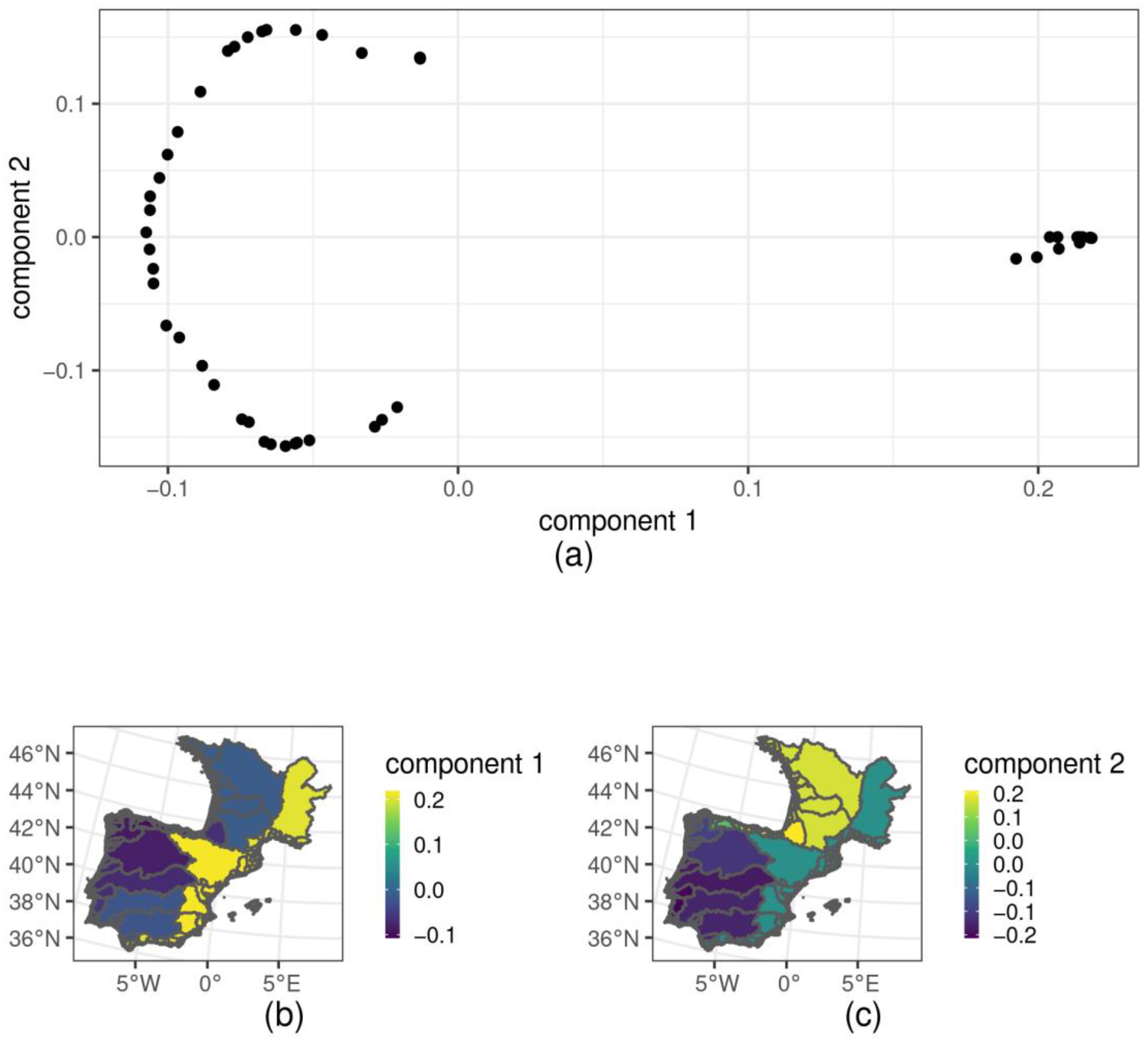
The PCA (Figure 2) showed three main clusters of river basins. The first axis separated the Mediterranean basins (positive values) from the Atlantic river basins (negative values). The second axis corresponded to a latitudinal gradient on the Atlantic coast. These two first axes represented 59% of the total inertia.
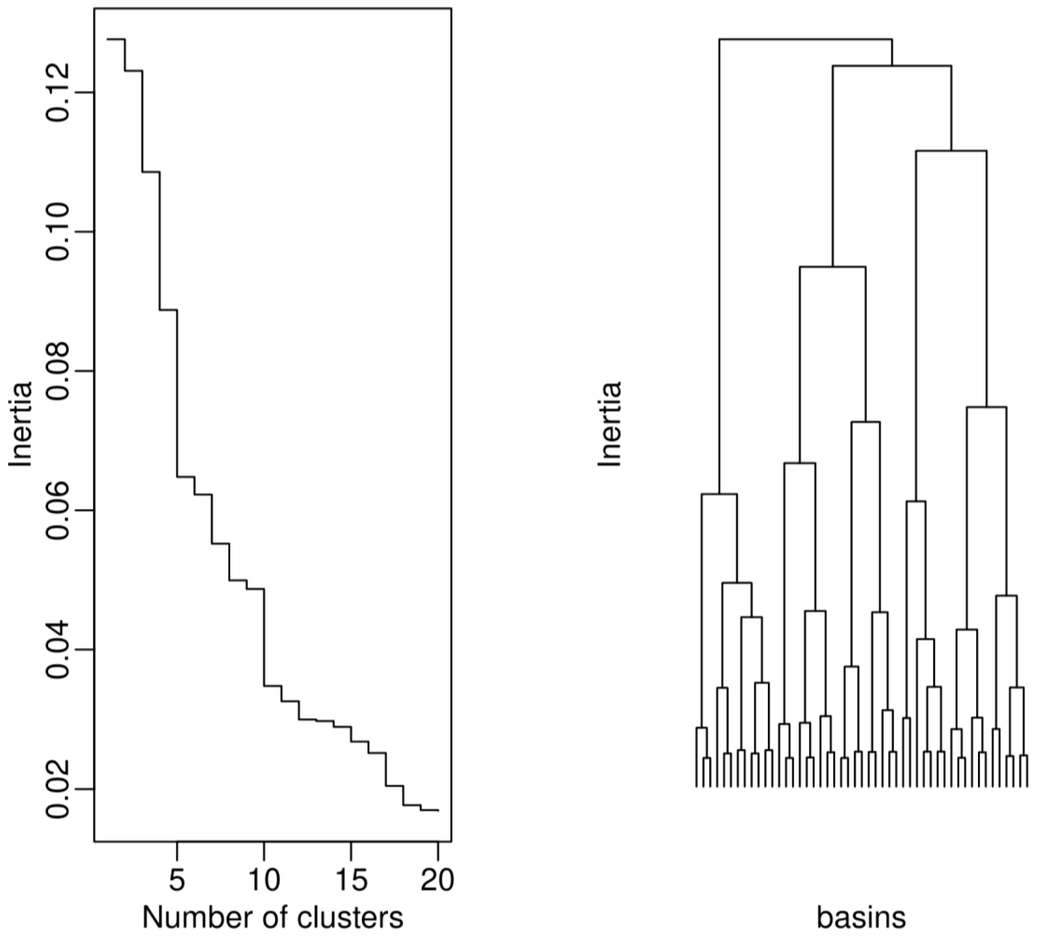
The diagram of the inertia gain of the clustering suggested the partitioning of the basins into three to five groups (Figure 3 and Figure S4).
Figure 1 shows the map resulting from the partitioning of four groups: the first zone corresponds to the French coast surrounding the Bay of Biscay (ATL_F) and is separated from the second zone corresponding to the Cantabrian Sea (CANT) at Cap Breton Canyon. The third group corresponds to the Atlantic coast of the Iberian Peninsula (ATL_IB), and the fourth group corresponds to the Mediterranean area (MED). The partitioning into three groups consists of merging the CANT and ATL_F zones (leading to a large Bay of Biscay zone). In the partitioning into five groups, the ATL_IB zone is split into two zones at Lisbon. In this last situation, only one relative time series of abundance (GuadG, Figure 1) would have been available for the zone corresponding to the south-western part of the Iberian Peninsula, so this configuration was rejected because the lack of data would not allow for the application of GEREM. The same applied to any number of zones larger than 5.
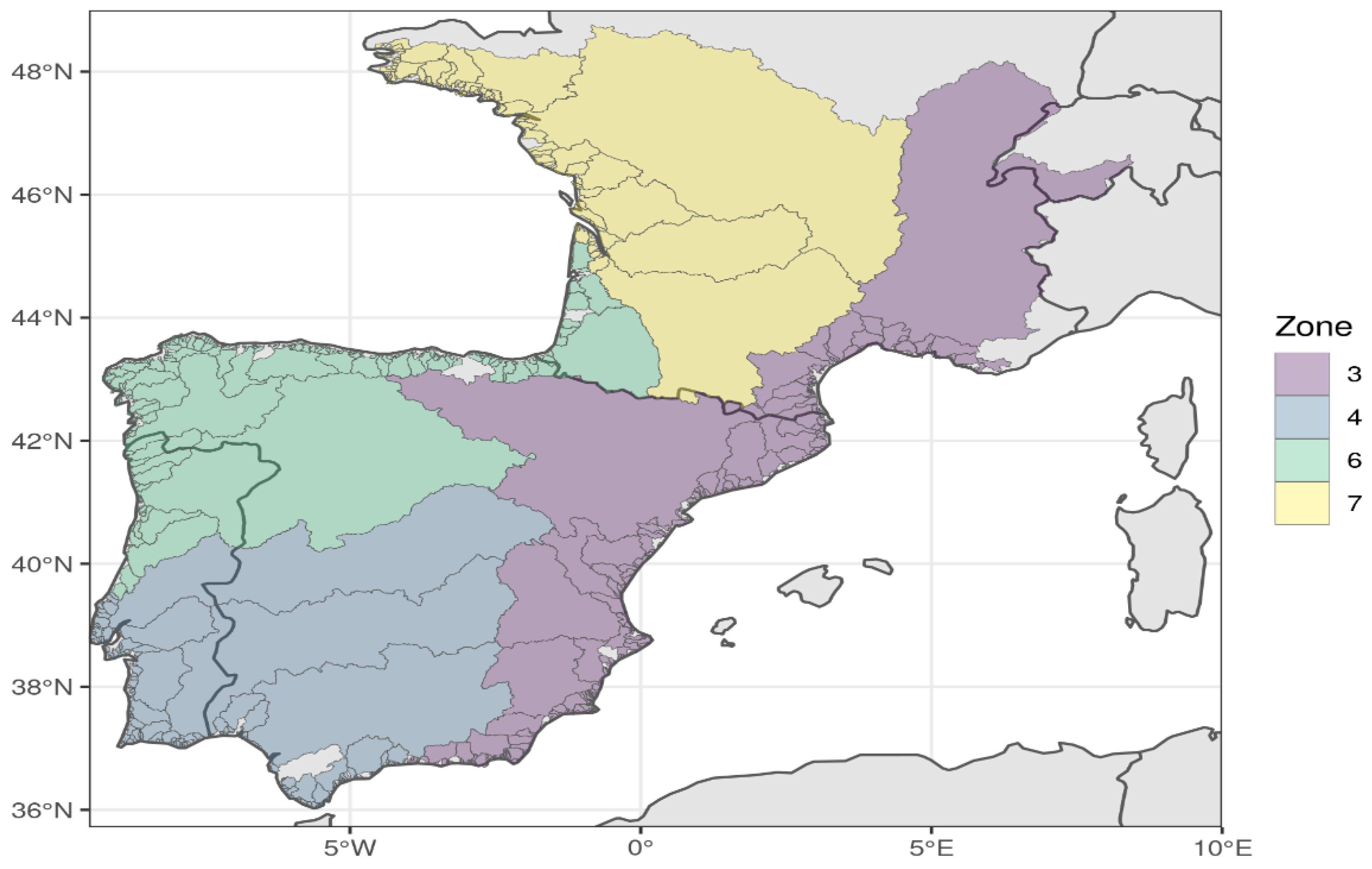
The maps of environmental variables are presented in the supplementary material (Figures S2 and S3). The regression tree of these environmental variables led to slight differences from the stakeholder classifications (Figure 4). The ATL_F zone is almost similar except that its southern border is slightly more to the north in the regression tree than in the expert opinion map. The same stands for the MED zone, whose border lies slightly eastward compared to that in the stakeholder opinion. However, stakeholders were aware of the presence of the Gibraltar Strait and Cap Breton Canyon, two features that were not taken into account in the regression tree of environmental variables. Then, the regression tree produced two additional zones: a zone that corresponds to the CANT zone and integrates part of the ATL_IB zone (the separation between CANT and ATL_IB was retrieved if we extended the depth of the regression tree). Then, the last zone is similar to the 5th zone that was proposed by stakeholders but was not kept because of the absence of available time series.
A dynamic factor analysis [48] confirmed that all available recruitment time series displayed very similar temporal trends (not presented here; [49]), so the assumption of similar trends within zones is not challenged. Therefore, after stakeholder validation, we decided to use the configuration with four zones: ATL_F, CANT, ATL_IB and MED (Figure 1).

3.2. Opinions on the Exploitation Rates and Resulting Priors

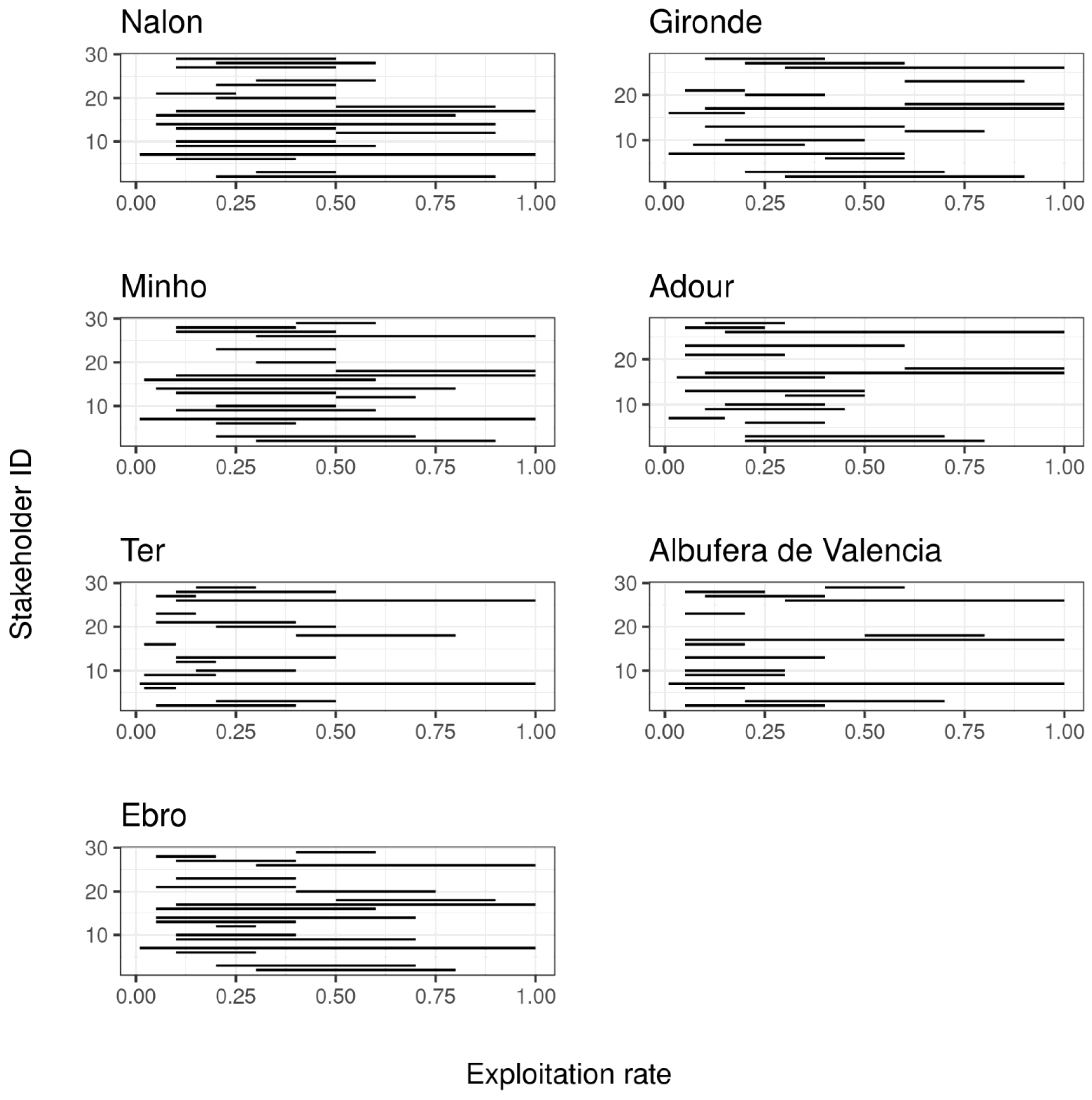
After the second stage of the questionnaires, 20 stakeholders expressed opinions about exploitation rates in at least one basin (26 persons attended the presential workshop in November 2018 for the first round of questionnaire: 13 scientists, 4 fishermen representatives, 5 managers and 1 NGO). Their opinions were contrasting (Figure 5). The bounds were large for all rivers, but this was consistent with the objective of the exercise of only limiting impossible values rather than providing precise estimates.
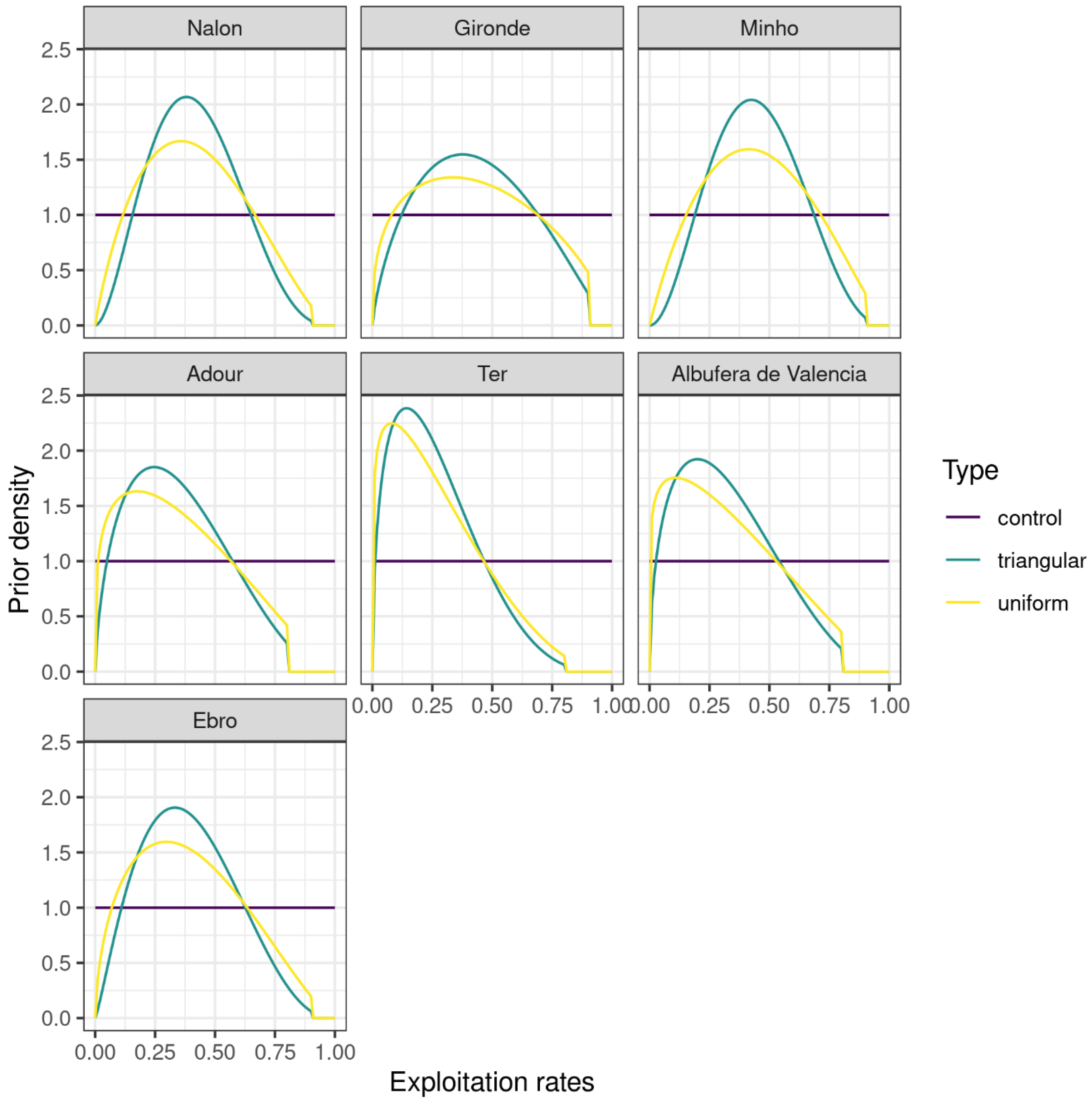
Despite the large bounds in the stakeholder opinions, some differences were visible among the compromise priors (Figure 6). The Gironde priors were the widest, while the Ter River had priors favouring the lowest exploitation rates. The difference between the “triangular” and “uniform” priors was limited, although “triangular” priors were slightly more informative than “uniform” priors, as seen by the higher probability densities.
Temporal trends in recruitment, model fits to observations and the effect of expert-based priors.
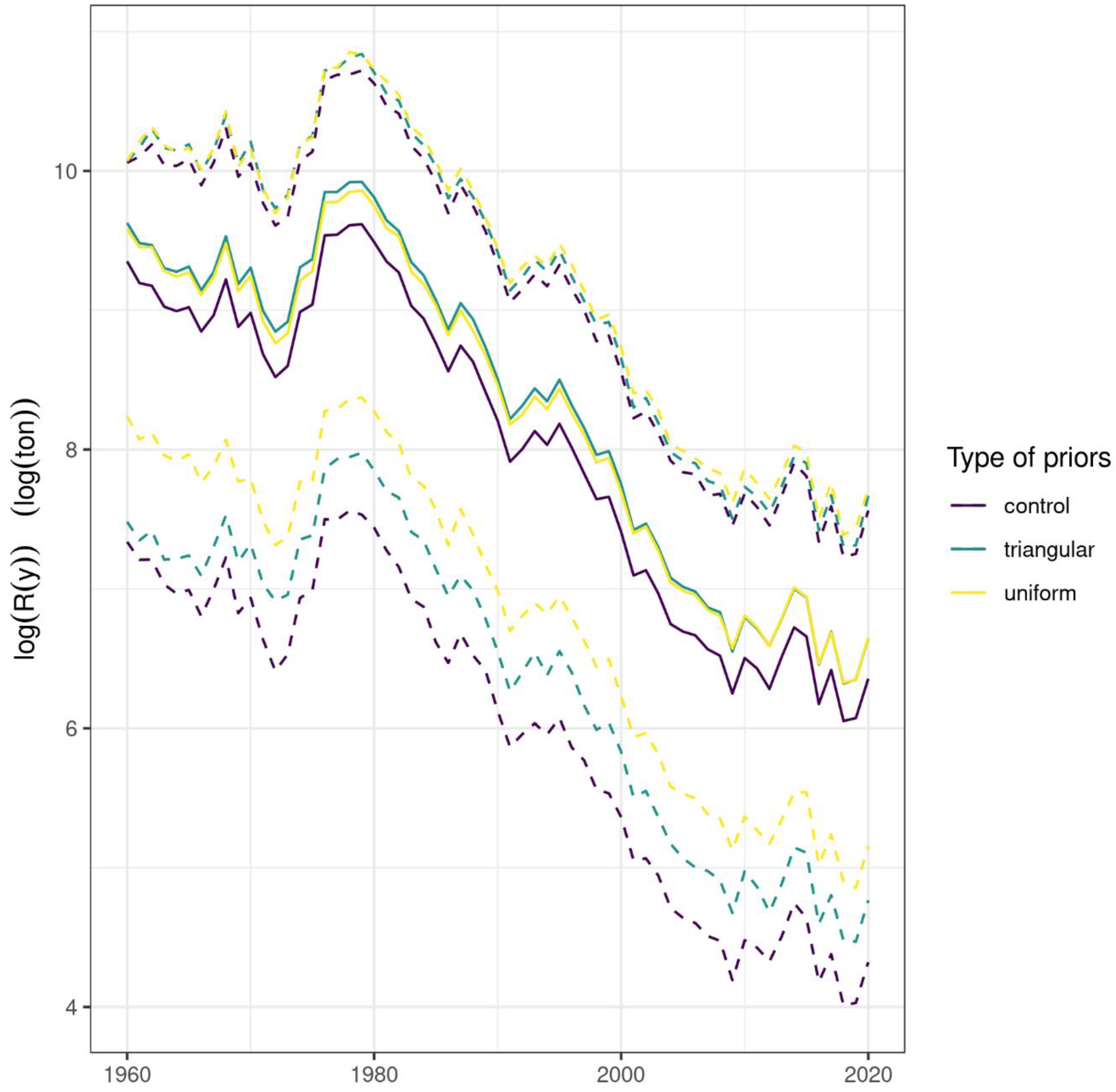
GEREM confirms the decline in recruitment since the early 1980s, regardless of whether stakeholders’ opinions are taken into account (Figure 7). All priors provide similar results. However, the stakeholder-based priors lead to slightly higher recruitment estimates: stakeholders-based priors favoured smaller exploitation rates than uniform priors (Figure 6), and since recruitment is assumed to be proportional to the commercial catches divided by the exploitation rate, a smaller exploitation mathematically leads to a higher recruitment.
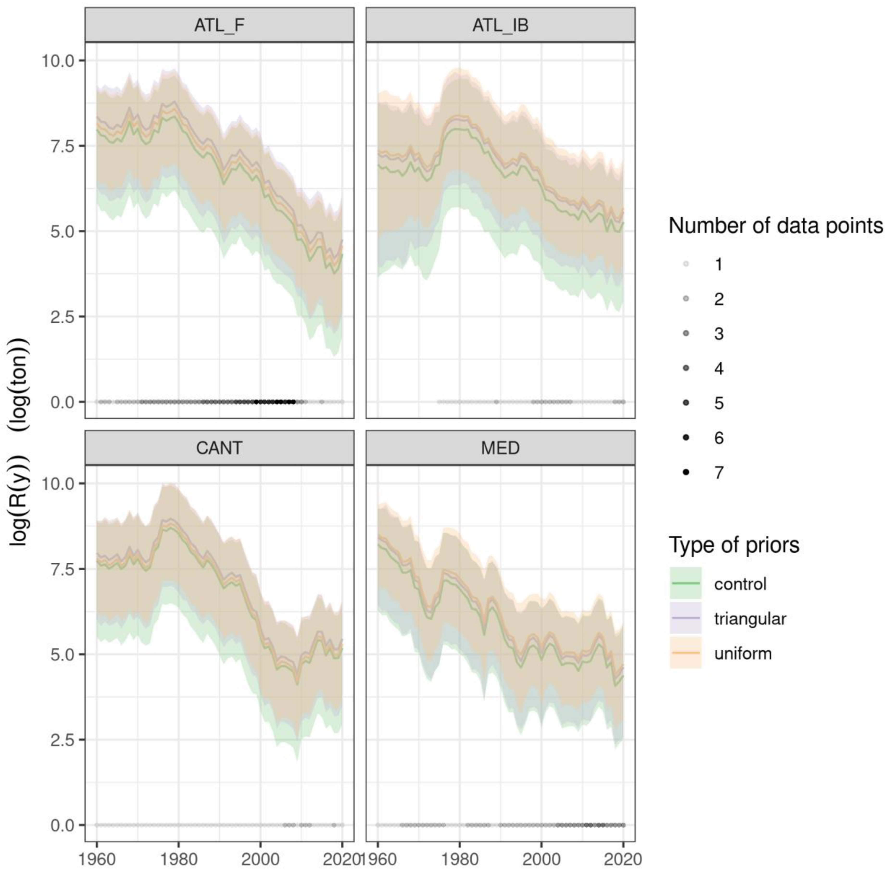
When analysing the results on the zone scale, several things can be noted (Figure 8). First, while all zones displayed a decreasing trend in recruitment from the 1980s to the early 2010s, the decrease in ATL_F was maintained to date, while recruitment appeared to stabilise in the other zones after 2010. However, the trend in ATL_F is based on a single time series of recruitment (GirScG) since the upkeep of French fishery-based time series ended after the implementation of the French Eel Management Plan [50]. Similarly, a decrease was estimated in MED during the 1960s; however, these estimates were based only on two fishery-based time series (Ebro and Albufera de Valencia). As before, the use of different priors did not lead to major differences in the temporal trends. However, in the case of ATL_F and ATL_IB, the estimations of recruitment were higher when stakeholder opinions were taken into account. In addition, in the case of ATL_F, the recruitment estimates were higher when using the “triangular” priors than when using the “uniform” priors.
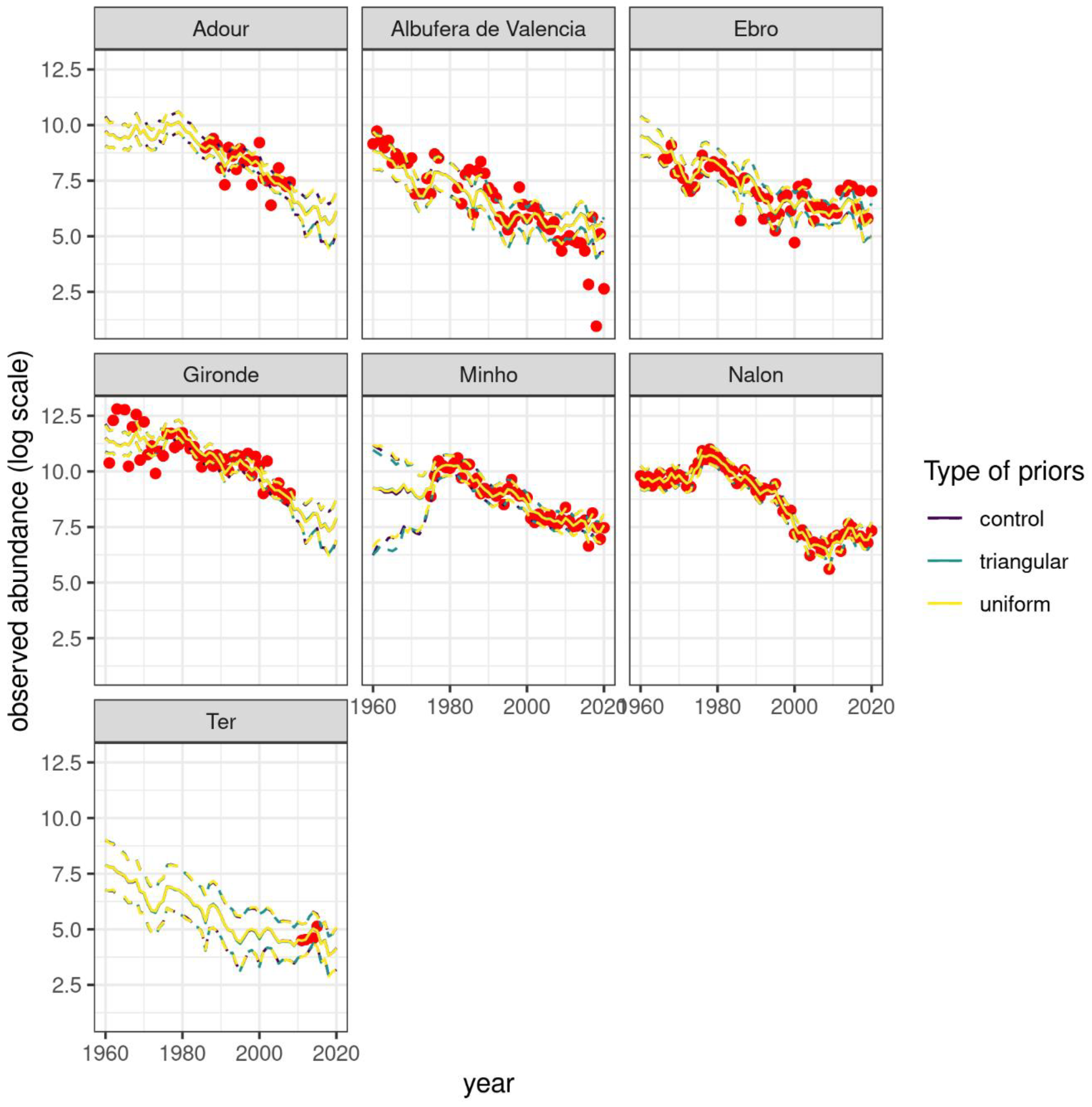
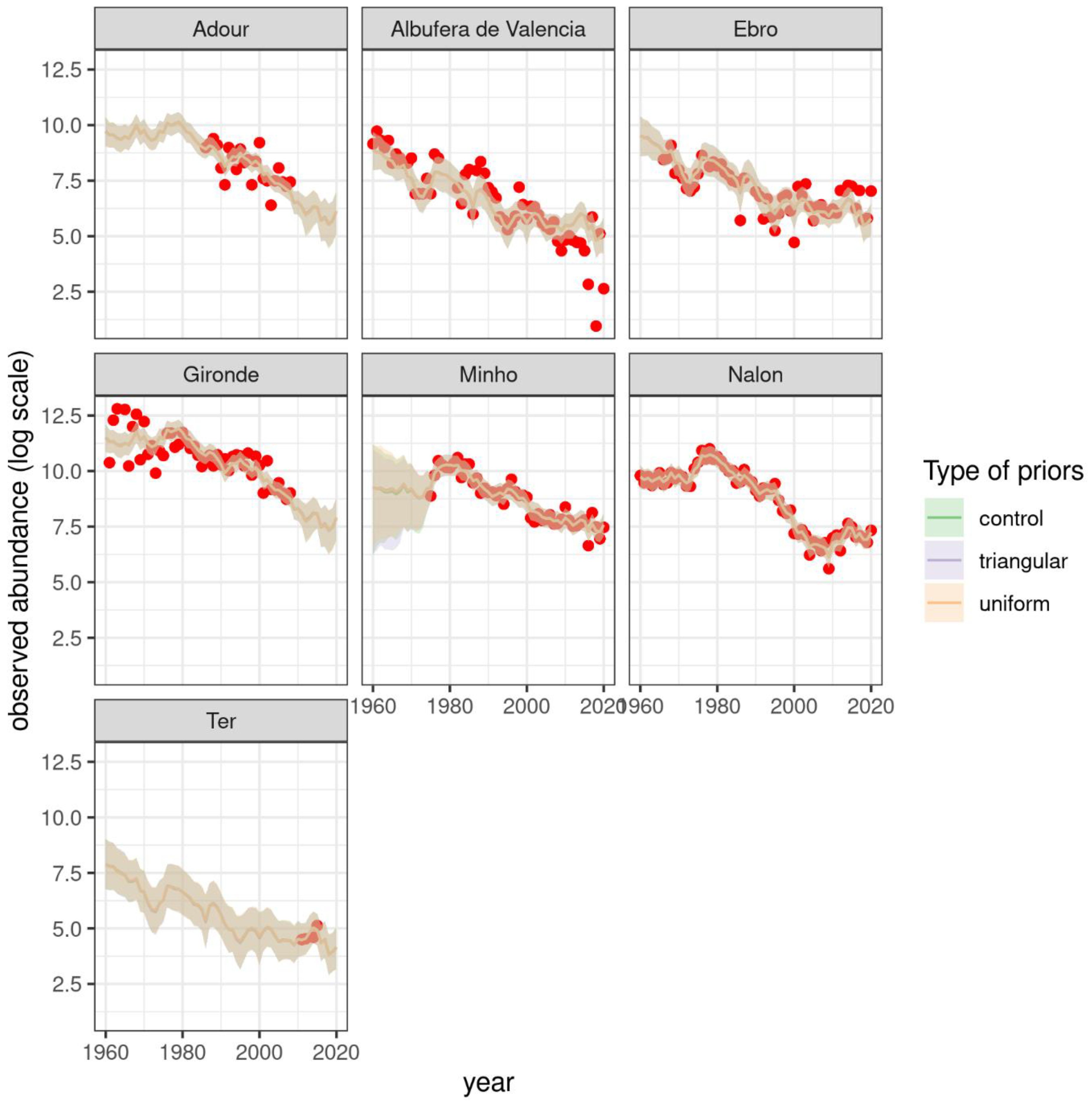
The results can also be displayed on the river basin scale and compared with the observations: the fits are very good and are similar among the types of priors (Figure 9).
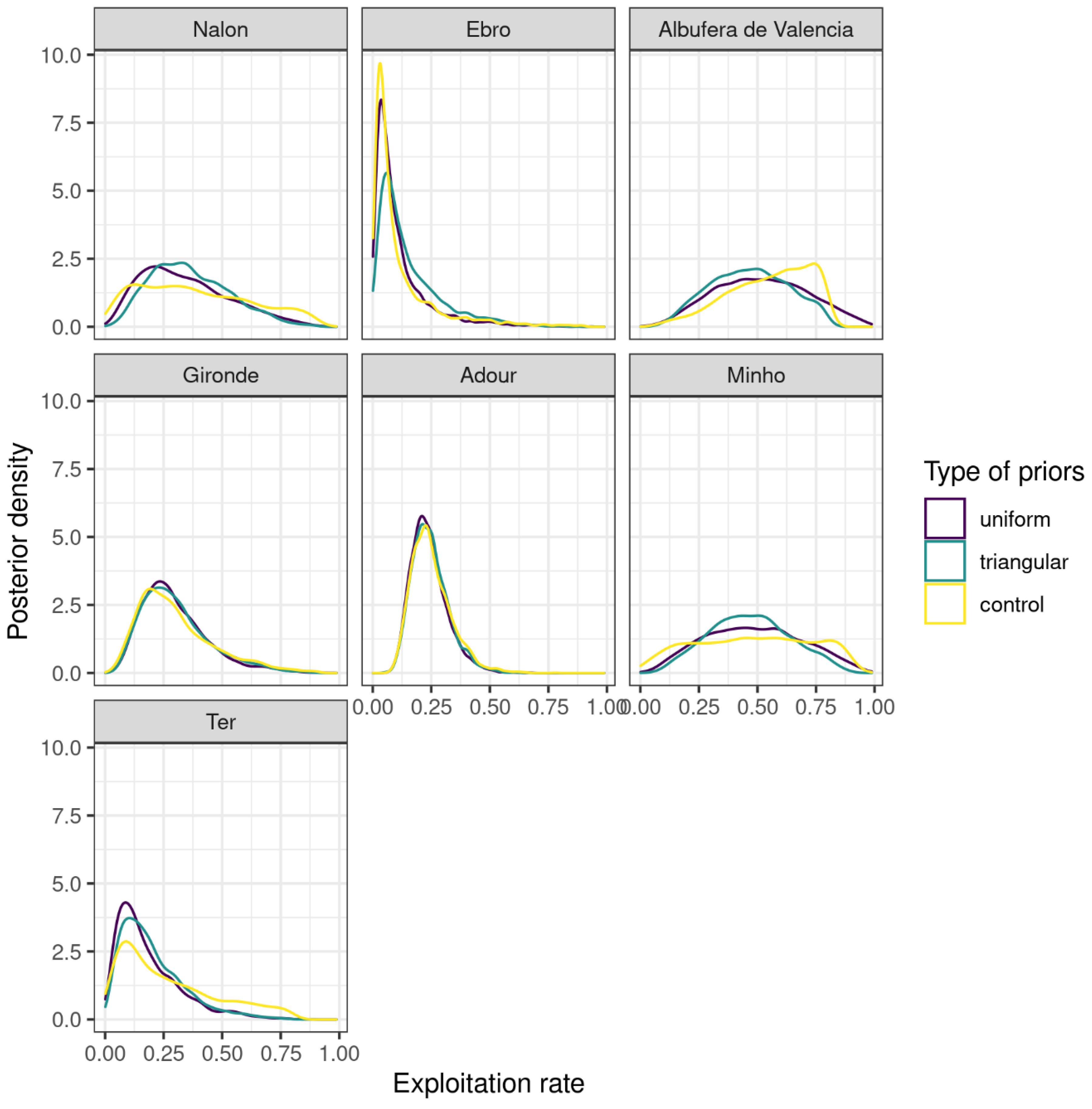
The posterior distributions of scaling factors qi (Equation (1)), i.e., the exploitation rates (see Section 2.5), are also similar regardless of the type of priors used, especially for the Gironde estuary and Adour River (Figure 10). However, some slight differences were observed if we compared the posterior distribution obtained with either the “control” prior or with the stakeholder-based priors. For example, the probability densities of the very low and high exploitation rates in the Minho basin were almost zero when the stakeholder-based priors, i.e., “uniform” and “triangular” priors, were used. In the Albufera de Valencia lagoon, using stakeholder-based priors led to the estimation of lower exploitation rates.

4. Discussion

4.1. Involving Stakeholders in Model Construction

Participatory modelling has been proposed as an important step in overcoming misunderstandings among stakeholders, rebuilding trust and achieving good governance in fisheries management [7]. In this context, this article presents an innovative exercise to involve stakeholders in the parametrisation of a complex model to increase their commitment and confidence in the approach and to achieve the production of a common assessment tool for the European eel in south-western Europe. This question of confidence in complex models as tools used to support fisheries management is crucial, and there is a need to improve transparency regarding model assumptions and uncertainties as well as a need to improve the transfer of model results [12]. The approach used here addressed all these points. To involve stakeholders, it was necessary to present the model assumptions during different workshops, to clarify how these assumptions can affect the model results and to be transparent regarding how the stakeholders′ opinions can be used in the model. The Bayesian approach allowed for the rigorous quantification of the uncertainties, and comparisons of different types of priors allowed us to explore the effect of considering stakeholders′ opinions. In the article, we focused on the tuning of the model, but the transfer of the results is also a key issue for complex models [12]. In view of this, the most relevant indicators of the model were also discussed in a dedicated workshop in which a questionnaire was used to collect the expectations of the participants about a user friendly web application to display the results. This result in a first web app version which was shown in the previously mentioned Youtube video (https://www.youtube.com/watch?v=6KlhH6FDmBM, accessed on 19 April 2021). We will only be able to determine in the long term whether our participatory approach has reconstructed trust among actors. However, the coordinator of SUDOANG presented the preliminary results of the GEREM and EDA implementation, and the Spanish Ministry found the results and the overall approach interesting. Moreover, a questionnaire sent to participants just after the presentation of the first results showed that most of the participants, at least partially, understood the basis of the model (12 answers out of 16), were satisfied by the zone definition (12 answers out of 14) and were satisfied with their implications in the model construction (10 out of 13; the 3 others were moderately satisfied). Since most of the “negative” answers were still related to minor misunderstandings about the model assumptions, we produced a final YouTube video titled “GEREM in a nutshell”, which is visible online (https://t.co/HTPnW9oNz2?amp = 1, accessed on 19 April 2021.
Sudoang was based on a large diversity of partners (see supplementary material) with different functions: scientists, control forces, fishermen representatives, NGOs, management. With such a large panel, it was difficult to achieve a perfectly balanced panel of types of actors and nationalities at each step of the project. Moreover, in many situations, it was chosen to keep questionnaires anonymous to facilitate participation and avoid self-censorship. However, this can cause biases in our analysis since we cannot ensure that the respondents were representative of the project. However, a sign-in sheet was used at each meeting so that we were sure that each type of actor has the opportunity to answer and get feedback on the results. Moreover, it confirms that the response rate was quite good compared to the attendance rate.

4.2. DISTATIS and the Construction of Stakeholder-Based Priors: Two Relevant Methods Used to Collect Expert Opinion

The Bayesian framework allows for expert knowledge to be used to build informative priors. Here, we follow the approach of [41] to build priors through the analysis of questionnaires sent to stakeholders. The expressed opinions were heterogeneous and thus resulted in very large priors. This is due to the approach used here, in which we only asked the participants to eliminate impossible values, not to provide precise estimates. While this may result in a loss of information, it allowed for more participants to express their opinions and, consequently, to participate in the model construction.
Exploitation rate is not easy to estimate since, theoretically, it requires estimating the abundance of incoming glass eels, a quantity unavailable in most river basins. In this context, stakeholders could only make an estimate of the efficiency of the fishery given its characteristics. Moreover, the estimates which are available in a few river basins are very heterogeneous: more than 95% in the Vilaine River [51], from 15 to 20% in the Loire estuary and 1 to 30% in the Adour estuary [32].
Eliciting expert knowledge requires knowing (1) how the expert opinion will be used, (2) what quantity to elicit, (3) designing the process—here the questionnaire, (4) performing the elicitation and (5) translating the elicited information into a model. Here, the integration of the spatial structure and priors for exploitation rates has a direct use in model construction, so Steps (1), (2) and (5) are quite straightforward. However, the elicitation could have been let differently, for instance, in the future it may be possible to build more informative priors by trying to improve the consensus among participants, for example, by using a DELPHI approach [52,53], which involves several rounds of assessments and discussion among experts; however, this may lead to the loss of some “shy” stakeholders and the risk of overdominance by other stakeholders. Another way of narrowing down the expert opinion range would be to weight the experts, based on a questionnaire for which the answers are known. This weight could then be used when pooling together the different responses [54,55]. However, since our aim was to increase the commitment of experts, we feared that experts receiving too little weight would reject the approach.
The DISTATIS method [34] is a method that is generally used in sensory and consumer science. Here, this method proved to be very relevant when comparing the classification maps made by different stakeholders and was used to achieve a compromise map that allowed us to objectively subdivide the study area into a set of zones. In this exercise, stakeholders′ opinions showed a good level of consistency with environmental data. For the few participants who had chosen not to remain anonymous, it was possible to see how their maps were located within the “map of experts”. In the future, it will be possible to compare the maps drawn by different types of actors and to explore, for example, whether the perceptions of the study region are consistent among French, Portuguese and Spanish stakeholders.
The same zones were also used in the EDA model [27], which was utilised to assess silver eel escapement in the SUDOANG project. However, while recruitment is mostly affected by large-scale factors, eels are subjected to heterogeneous environmental conditions and anthropogenic pressures [16]. Therefore, it would be worthwhile in the future to renew the exercise by asking stakeholders to make new classifications based on not only on their perception of environmental factors in continental waters but also on their perception of human factors: pressures and administrative zoning.
Regarding more specifically the replication potential of the approach with the model GEREM, GEREM was already applied at the French level [28] and on the European scale [21]. In these two analyses, uninformative priors were used for scaling factors and expert knowledge was not accounted for in the zone definition. The possibility to use informative priors on the scaling possible factor makes the model even more flexible as the need for absolute estimates of recruitment in certain river basins becomes less critical: commercial catch data or trap counting are much more frequent than absolute estimates. In this context, the possibility to use the model for the American eel has been discussed [56] and first intents have been made to use GEREM in Japan for the Japanese eel (Yokouchi et al., unpublished).

4.3. The Effect of Incorporating Stakeholder Knowledge

Since most of the time series used in this exercise were already used by [21] and are annually used by [23], the resulting trend was very similar to those of previous studies and confirms a decline since the early 1980s. While stakeholders and environmental data suggested to split the zone ATL_IB into two zones (supplementary material Figure S4), it was not possible because of the lack of data in Southwestern Iberian Peninsula. This, combined with the large credibility intervals in some zones (including ATL_F in recent years), urges the implementation of new monitoring series. In this sense, the coordinated monitoring network implemented in the SUDOANG project appears especially relevant and may be used to fill this gap and provide consistent and comparable time series of abundance and biometry. This coordination is especially important since it is well known that inconsistencies in protocols can lead to biases in trend assessment [57].
The results obtained when using stakeholder-based priors were not very different from the results obtained with “control” priors. Obviously, this is due to the wideness of these priors, but this result also shows that stakeholders’ opinions were consistent with the data observations. The overall area trend and zone-scale trends were similar regardless of the type of priors used, although recruitment was slightly lower with the “control” priors. At the river basin level, this result also led to differences in the posterior distributions of exploitation rates. While it is unsurprising that the use of stakeholder-based priors did not change the posterior distribution of exploitation rates in river basins for which absolute time series of recruitment are also available (Gironde estuary and Adour River), differences were observed in some other rivers (e.g., the Minho River, Albufera de Valencia lagoon). The two procedures for constructing stakeholder-based priors led to similar priors (Figure 6) and consequently had very limited impacts on the results. However, we chose to remain very cautious in the construction of the priors. Some authors have recommended restricting the number of experts involved in the construction of priors to find a compromise between redundant information and a good representation of opinion inter-variability [58,59]. By limiting the number of stakeholders, we might have achieved more informative priors and would probably have obtained greater differences between the “triangular” and the “uniform” priors; however, this would require a non-anonymous questionnaire to obtain sufficient information with which to operate stakeholder selection.

4.4. Towards the Comparison of Recruitment and Escapement

The SUDOANG project will provide estimates of both recruitment through the use of GEREM [28] and escapement with EDA [27]. By doing so, managers will have comparable and consistent indicators of population statuses over the south-western European area. This is a step forward in fulfilling the need for the coordination of local assessments and to orchestrate initiatives among countries. Currently, we are still not able to carry out the exercise over the whole distribution area [20], but a roadmap has been established to achieve that goal [60].

Supplementary Materials

The following are available online at https://www.mdpi.com/article/10.3390/w13091136/s1, Figure S1: Example of map drawn by an expert during the kick-off meeting in Lisbon, Figure S2: Environmental conditions over the study area, Figure S3: Environmental conditions characterizing river basins, Figure S4: The Distatis analysis of maps produced by experts, Table S1: List of partners, An example of questionnaires on exploitation rate is also provided.

Author Contributions

Conceptualization, H.D., C.B., M.V., E.D., M.M. and P.L.; methodology, H.D., C.B., M.V. and P.L.; software, H.D. and M.V.; validation, H.D., C.B., M.V., E.D., M.M., P.L., M.K., C.A., C.F.D., I.D., L.Z. and L.B.; formal analysis, H.D. and M.V.; investigation, H.D., C.B., M.V., E.D., M.M., P.L., M.K., C.A., C.F.D., I.D., L.Z. and L.B.; resources, H.D., C.B., M.V., E.D., M.M., P.L., M.K., C.A., C.F.D., I.D., L.Z. and L.B.; data curation, H.D., C.B., M.V., E.D., M.M., P.L., M.K., C.A., C.F.D., I.D., L.Z. and L.B.; writing—original draft preparation, H.D. and M.V; writing—review and editing, H.D., C.B., M.V., E.D., M.M., P.L., M.K., C.A., C.F.D., I.D., L.Z. and L.B.; visualization, H.D. supervision, H.D.; project administration, E.D.; funding acquisition, H.D., C.B., M.V., E.D., P.L., M.K., C.A., C.F.D., I.D., L.Z. and L.B. All authors have read and agreed to the published version of the manuscript.

Funding

The SUDOANG project was funded by the Interreg Program Sudoe V (project SOE2/P5/E0617) through the European Regional Development Fund (ERDF).

Institutional Review Board Statement

No new monitoring data were collected for the purpose of this study.

Informed Consent Statement

Informed consent was obtained from all subjects involved in the study.

Data Availability Statement

The data presented in this study are available on request from the corresponding author. The data are not publicly available due to privacy of some data.

Acknowledgments

The SUDOANG project was funded by the Interreg Program Sudoe V. The authors are grateful to all SUDOANG beneficiaries and associate partners who contributed to the different workshops and answered the questionnaires.

Conflicts of Interest

The authors declare no conflict of interest.

References

  1. Smith, M.E. Chaos in Fisheries Management. Marit. Anthropol. Stud. 1990, 3, 1–13. [Google Scholar]
  2. de Vos, B.I.; van Tatenhove, J.P.M. Trust Relationships Between Fishers and Government: New Challenges for the Co-Management Arrangements in the Dutch Flatfish Industry. Mar. Policy 2011, 35, 218–225. [Google Scholar] [CrossRef]
  3. Glenn, H.; Tingley, D.; Sánchez Maroõ, S.; Holm, D.; Kell, L.; Padda, G.; Runar Edvardsson, I.; Asmundsson, J.; Conides, A.; Kapiris, K.; et al. Trust in the Fisheries Scientific Community. Mar. Policy 2012, 36, 54–72. [Google Scholar] [CrossRef]
  4. Planque, B.; Mullon, C. Modelling Chance and Necessity in Natural Systems. ICES J. Mar. Sci. 2020, 77, 1573–1588. [Google Scholar] [CrossRef]
  5. Glaser, S.M.; Fogarty, M.J.; Liu, H.; Altman, I.; Hsieh, C.-H.; Kaufman, L.; MacCall, A.D.; Rosenberg, A.A.; Ye, H.; Sugihara, G. Complex Dynamics May Limit Prediction in Marine Fisheries. Fish Fish. 2014, 15, 616–633. [Google Scholar] [CrossRef]
  6. Wilson, J.A.; Townsend, R.; Kelban, P.; McKay, S.; French, J. Managing Unpredictable Resources: Traditional Policies Applied to Chaotic Populations. Ocean Shorel. Manag. 1990, 13, 179–197. [Google Scholar] [CrossRef]
  7. Röckmann, C.; Ulrich, C.; Dreyer, M.; Bell, E.; Borodzicz, E.; Haapasaari, P.; Hauge, K.H.; Howell, D.; Mäntyniemi, S.; Miller, D.; et al. The Added Value of Participatory Modelling in Fisheries Management—What Has Been Learnt? Mar. Policy 2012, 36, 1072–1085. [Google Scholar] [CrossRef] [Green Version]
  8. Planque, B.; Mullon, C.; Arneberg, P.; Eide, A.; Fromentin, J.-M.; Heymans, J.J.; Hoel, A.H.; Niiranen, S.; Ottersen, G.; Sandø, A.B.; et al. A Participatory Scenario Method to Explore the Future of Marine Social-Ecological Systems. Fish Fish. 2019, 20, 434–451. [Google Scholar] [CrossRef]
  9. Johannes, R.E.; Freeman, M.M.R.; Hamilton, R.J. Ignore Fishers’ Knowledge and Miss the Boat. Fish Fish. 2000, 1, 257–271. [Google Scholar] [CrossRef]
  10. Pita, P.; Fernández-Vidal, D.; García-Galdo, J.; Muíño, R. The Use of the Traditional Ecological Knowledge of Fishermen, Cost-Effective Tools and Participatory Models in Artisanal Fisheries: Towards the Co-Management of Common Octopus in Galicia (NW Spain). Fish. Res. 2016, 178, 4–12. [Google Scholar] [CrossRef]
  11. Pita, C.; Pierce, G.J.; Theodossiou, I. Stakeholders’ Participation in the Fisheries Management Decision-Making Process: Fishers’ Perceptions of Participation. Mar. Policy 2010, 34, 1093–1102. [Google Scholar] [CrossRef]
  12. Lehuta, S.; Girardin, R.; Mah’evas, S.; Travers-Trolet, M.; Vermard, Y. Reconciling Complex System Models and Fisheries Advice: Practical Examples and Leads. Aquat. Living Resour. 2016, 29, 208. [Google Scholar] [CrossRef]
  13. Schmidt, J. Breeding Places and Migrations of the Eel. Nature 1923, 111, 51–54. [Google Scholar] [CrossRef] [Green Version]
  14. Tesch, F.W. The Eel; Blackwell Publishing: Oxford, UK, 2003. [Google Scholar]
  15. Als, T.D.; Hansen, M.M.; Maes, G.E.; Castonguay, M.; Riemann, L.; Aarestrup, K.; Munk, P.; Sparholt, H.; Hanel, R.; Bernatchez, L. All Roads Lead to Home: Panmixia of European Eel in the Sargasso Sea. Mol. Ecol. 2011, 20, 1333–1346. [Google Scholar] [CrossRef] [PubMed]
  16. Dekker, W. The Fractal Geometry of the European Eel Stock. ICES J. Mar. Sci. 2000, 57, 109–121. [Google Scholar] [CrossRef]
  17. Drouineau, H.; Rigaud, C.; Daverat, F.; Lambert, P. Eveel (Evolutionary Ecology Based Model for Eel): A Model to Explore the Role of Phenotypic Plasticity as an Adaptive Response of Three Temperate Eels (Anguilla Anguilla, A. Japonica and A. Rostrata) to Spatially Structured Environments. Can. J. Fish. Aquat. Sci. 2014, 71, 1561–1571. [Google Scholar] [CrossRef]
  18. Kettle, A.J.; Asbjørn Vøllestad, L.; Wibig, J. Where Once the Eel and the Elephant Were Together: Decline of the European Eel Because of Changing Hydrology in Southwest Europe and Northwest Africa? Fish Fish. 2011, 12, 380–411. [Google Scholar] [CrossRef]
  19. Vøllestad, L.A. Geographic Variation in Age and Length at Metamorphosis of Maturing European Eel—Environmental Effects and Phenotypic Plasticity. J. Anim. Ecol. 1992, 61, 41–48. [Google Scholar] [CrossRef]
  20. Dekker, W. Management of the Eel Is Slipping Through Our Hands! Distribute Control and Orchestrate National Protection. ICES J. Mar. Sci. 2016, 73, 2442–2452. [Google Scholar] [CrossRef] [Green Version]
  21. Bornarel, V.; Lambert, P.; Briand, C.; Beaulaton, L.; Antunes, C.; Belpaire, C.; Cicotti, E.; Evans, D.; Diaz, E.; Diserud, O.H.; et al. Modelling the Recruitment of European Eel (Anguilla Anguilla) Throughout Its European Range. ICES J. Mar. Sci. 2018, 75, 541–552. [Google Scholar] [CrossRef]
  22. Dekker, W. Did Lack of Spawners Cause the Collapse of the European Eel, Anguilla Anguilla? Fish Manag. Ecol. 2003, 10, 365–376. [Google Scholar] [CrossRef]
  23. ICES Joint EIFAAC/ICES/GFCM Working Group on Eels (WGEEL); ICES Scientific Reports Issue 50; ICES: Bergen, Norway, 2019; Volume 1, p. 177.
  24. Pike, C.; Crook, V.; Gollock, M. Anguilla anguilla. In The IUCN Red List of Threatened Species 2020: E.T60344A152845178. 2020. Available online: http://www.iucnredlist.org (accessed on 19 April 2021).
  25. Drouineau, H.; Durif, C.; Castonguay, M.; Mateo, M.; Rochard, E.; Verreault, G.; Yokouchi, K.; Lambert, P. Freshwater Eels: A Symbol of the Effects of Global Change. Fish Fish. 2018, 19, 903–930. [Google Scholar] [CrossRef] [Green Version]
  26. Feunteun, E. Management and Restoration of European Eel Population (Anguilla Anguilla): An Impossible Bargain. Ecol. Eng. 2002, 18, 575–591. [Google Scholar] [CrossRef]
  27. Briand, C.; Chapon, P.M.; Beaulaton, L.; Drouineau, H.; Lambert, P. Eel Density Analysis (EDA 2.2.1) Escapement of Silver Eels (Anguilla anguilla) from French Rivers—Report 2018; EPTB Vilaine–Agence Française de la Biodiversité-Inra-Irstea: La Roche-Bernard, France, 2018. [Google Scholar]
  28. Drouineau, H.; Beaulaton, L.; Lambert, P.; Briand, C. GEREM (Glass-Eel Recruitment Estimation Model): A Model to Estimate Glass-Eel Recruitment at Different Spatial Scales. Fish. Res. 2016, 174, 68–80. [Google Scholar] [CrossRef] [Green Version]
  29. Dekker, W. Thematic Overview. In Monitoring of Glass Eel Recruitment; Report C007/02-WD; RIVO-Netherlands Institute for Fisheries Research: Ijmuiden, The Netherlands, 2002; p. 256. [Google Scholar]
  30. Aranburu, A.; Diaz, E.; Briand, C. Glass Eel Recruitment and Exploitation in a South European Estuary (Oria Bay of Biscay). ICES J. Mar. Sci. 2016, 73, 111–121. [Google Scholar] [CrossRef] [Green Version]
  31. Beaulaton, L.; Briand, C. Effect of Management Measures on Glass Eel Escapement. ICES J. Mar. Sci. 2007, 64, 1402–1413. [Google Scholar] [CrossRef] [Green Version]
  32. Bru, N.; Prouzet, P.; Lejeune, M. Daily and Seasonal Estimates of the Recruitment and Biomass of Glass Eels Runs (Anguilla Anguilla) and Exploitation Rates in the Adour Open Estuary (Southwestern France). Aquat. Living Resour. 2009, 22, 509–523. [Google Scholar] [CrossRef] [Green Version]
  33. de Catalunya, G. Plan de Gestión de La Anguila Europea—Cataluńa; Generalitat de Catalunya: Barcelona, Spain, 2012.
  34. Abdi, H.; O’Toole, A.J.; Valentin, D.; Edelman, B. DISTATIS: The Analysis of Multiple Distance Matrices. In Proceedings of the IEEE Conference on Computer Vision and Pattern Recognition, CVPR Workshops 2005, San Diego, CA, USA, 21–23 September 2005; p. 42. [Google Scholar]
  35. Abdi, H.; Valentin, D.; Chollet, S.; Chrea, C. Analyzing Assessors and Products in Sorting Tasks: DISTATIS, Theory and Applications. Food Qual. Prefer. 2007, 18, 627–640. [Google Scholar] [CrossRef]
  36. Beaton, D.; Fatt, C.C.; Abdi, H. DistatisR: DiSTATIS Three Way Metric Multidimensional Scaling; VNU Publishing House: London, UK, 2019. [Google Scholar]
  37. Hijmans, R.J.; Cameron, S.E.; Parra, J.L.; Jones, P.G.; Jarvis, A. Very High Resolution Interpolated Climate Surfaces for Global Land Areas. Int. J. Climatol. 2005, 25, 1965–1978. [Google Scholar] [CrossRef]
  38. ICES Workshop on the Temporal Migration Patterns of European Eel (WKEELMIGRATION); ICES Scientific Reports Volume 2, Issue 205; ICES: Copenhagen, Denmark, 2020; p. 109.
  39. De’Ath, G. Multivariate Regression Trees: A New Technique for Modelling Species-Environment Relationships. Ecology 2002, 83, 1105–1117. [Google Scholar]
  40. Hothorn, T.; Zeileis, A. Partykit: A Modular Toolkit for Recursive Partytioning in R. J. Mach. Learn. Res. 2015, 16, 3905–3909. [Google Scholar]
  41. Tableau, A.; Drouineau, H.; Delpech, C.; Pierre, M.; Lobry, J.; Le Pape, O.; Breine, J.; Lepage, M. A Fish-Based Index of Estuarine Ecological Quality Incorporating Information from Both Scientific Fish Survey and Experts Knowledge. Ecol. Indic. 2013, 32, 147–156. [Google Scholar] [CrossRef] [Green Version]
  42. Briand, C.; Fatin, D.; Feunteun, E.; Fontenelle, G. Estimating the Stock of Glass Eels in an Estuary by Mark-Recapture Experiments Using Vital Dyes. Bull. Fr. Pêche Piscic. 2005, 378–379, 23–46. [Google Scholar] [CrossRef] [Green Version]
  43. Drouineau, H.; Rigaud, C.; Laharanne, A.; Fabre, R.; Bau, F.; Baran, P. Assessing the Efficiency of an Eel Ladder and Trap Using Tag-Recaptures Data and a Bayesian Model. In Proceedings of the 6th World Fisheries Congess, Edinburgh, UK, 7–11 May 2012. [Google Scholar]
  44. Mateo, M.; Briand, C.; Beaulaton, L.; Drouineau, H. GT1—Produit 1.1; Atlas Sudoang: La Roche Bernard, France; Girona, Spain; Lisbon, Portugal, 2020. [Google Scholar]
  45. Pella, H.; Lejot, J.; Lamouroux, N.; Snelder, T. Le réseau hydrographique théorique (RHT) français et ses attributs environnementaux. Géomorphol. Relief Process. Environ. 2012, 18, 317–336. [Google Scholar] [CrossRef] [Green Version]
  46. Plummer, M. JAGS: A Program for Analysis of Bayesian Graphical Models Using Gibbs Sampling. In Proceedings of the 3rd International Workshop on Distributed Statistical Computing, Vienna, Austria, 20–22 March 2003. [Google Scholar]
  47. Denwood, M.J. Runjags: An R Package Providing Interface Utilities, Model Templates, Parallel Computing Methods and Additional Distributions for MCMC Models in JAGS. J. Statist. Softw. 2016, 71, 1–25. [Google Scholar] [CrossRef] [Green Version]
  48. Zuur, A.F.; Fryer, R.J.; Jolliffe, I.T.; Dekker, R.; Beukema, J.J. Estimating Common Trends in Multivariate Time Series Using Dynamic Factor Analysis. Environmetrics 2003, 14, 665–685. [Google Scholar] [CrossRef] [Green Version]
  49. Drouineau, H. GT3—Délivrable E3.1.1: Inventaire Des Données Disponibles Sur Le Recrutement Pour Application Du Modèle GEREM; Atlas Sudoang: La Roche Bernard, France; Girona, Spain; Lisbon, Portugal, 2019. [Google Scholar]
  50. Ministère de l’Ecologie, de l’Energie, du Developpement durable et de l’Aménagement du Territoire; Onema. Ministère de l’Agriculture et de la Pêche Plan de Gestion Anguille de La France—Application Du Règlement (CE) 1100/2007 Du 18 Septembre 2007—Volet National; Ministère de l’Ecologie, de l’Energie, du Développement Durable et de la Mer, en Charge des Technologies Vertes et des Négociations sur le Climat, Onema, Ministère de l’Alimentation, de l’Agriculture et de la Pêche: Paris, France, 2010.
  51. Briand, C.; Fatin, D.; Fontenelle, G.; Feunteun, E. Estuarine and fluvial recruitment of the European glass eel, Anguilla anguilla, in an exploited Atlantic estuary. Fish. Manag. Ecol. 2003, 10, 377–384. [Google Scholar] [CrossRef]
  52. Jacobs, R.A. Methods for Combining Experts’ Probability Assessments. Neural Comput. 1995, 7, 867–888. [Google Scholar] [CrossRef]
  53. Linstone, H.A.; Turoff, M. Introduction to the Delphi Method: Techniques and Applications. Delphi Method Tech. Appl. 1975, 3–12. [Google Scholar]
  54. Cooke, R. Experts in Uncertainty: Opinion and Subjective Probability in Science; Oxford University Press: Oxford, UK, 1991. [Google Scholar]
  55. Martin, T.G.; Burgman, M.A.; Fidler, F.; Kuhnert, P.M.; Low-Choy, S.; McBride, M.; Mengersen, K. Eliciting expert knowledge in conservation science. Conserv. Biol. 2012, 26, 29–38. [Google Scholar] [CrossRef] [Green Version]
  56. Cairns, D.K.; Avery, T.S.; Benchetrit, J.; Bornarel, V.; Casselman, J.M.; Castonguay, M.; Crow, S.K.; Dorow, M.; Drouineau, H.; Frankowski, J.; et al. Methods and data sources to support American eel population analysis. DFO Can. Sci. Advis. Sec. Res. Doc. 2020, in press. [Google Scholar]
  57. Pasquaud, S.; Brind’Amour, A.; Berthelé, O.; Girardin, M.; Elie, P.; Boët, P.; Lepage, M. Impact of the Sampling Protocol in Assessing Ecological Trends in an Estuarine Ecosystem: The Empirical Example of the Gironde Estuary. Ecol. Indic. 2012, 15, 18–29. [Google Scholar] [CrossRef] [Green Version]
  58. Clemen, R.T.; Winkler, R.L. Limits for the Precision and Value of Information from Dependent Sources. Oper. Res. 1985, 33, 427–442. [Google Scholar] [CrossRef]
  59. Ferrell, W.R. Combining individual judgments. In Behavioral Decision Making; Springer: Boston, MA, USA, 1985; pp. 111–145. [Google Scholar]
  60. ICES Report of Workshop on the Future of Eel Advice (WKFEA); ICES Scientific Report; ICES: Copenhagen, Denmark, 2021; Volume 3.
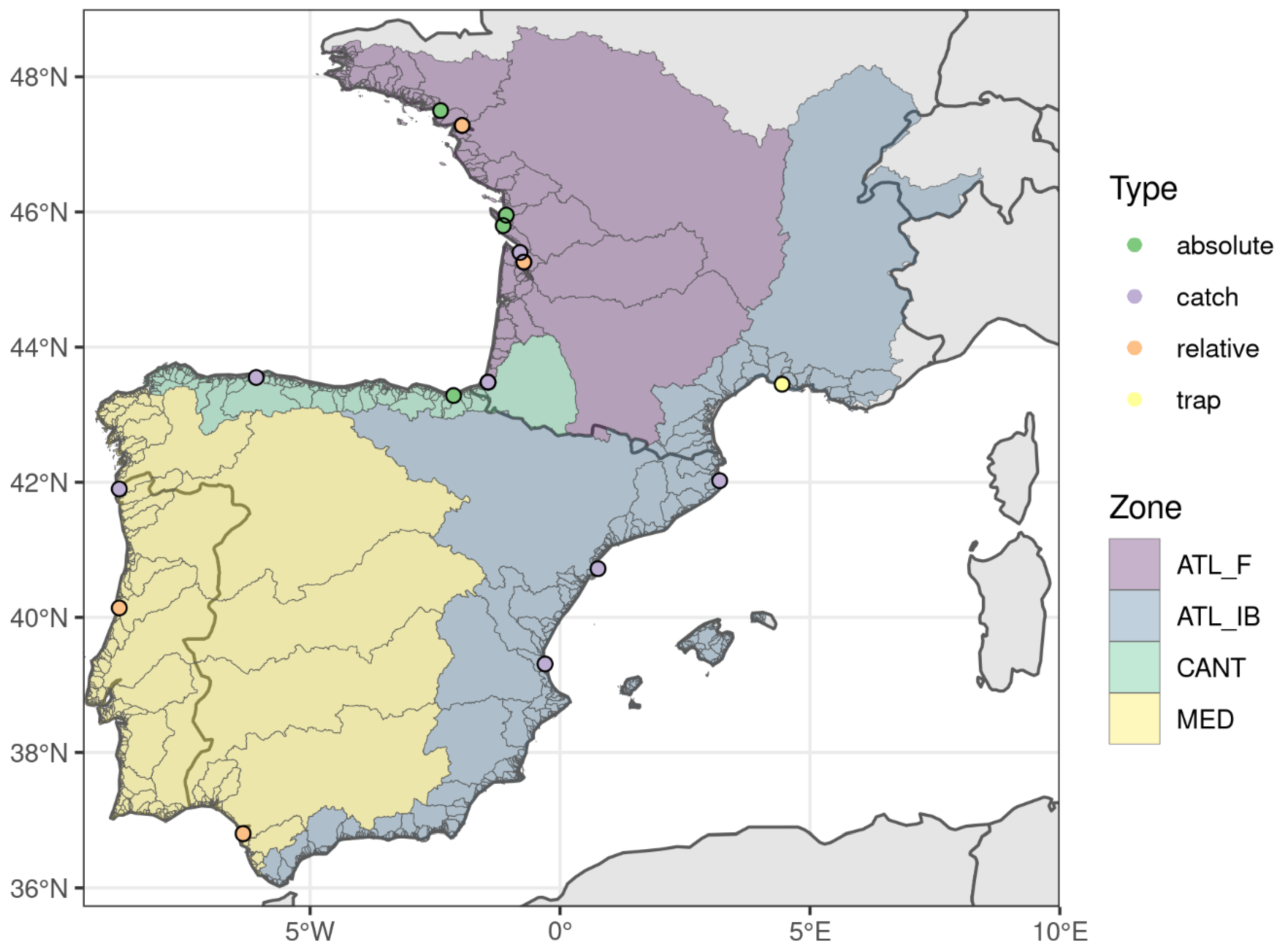
Figure 1. Maps of available time series (dots) and zone definitions (colored polygons) used in GEREM. The colors of the dots indicate the type of time series. The zones were defined based on expert knowledge (see Section 2.4 and Section 3.1).
Water 13 01136 g001
Figure 2. Positions of the basins in the first 2 components of the compromise space of stakeholder classifications from the DISTATIS method (a) and spatial representation of the coordinates of the basins in this diagram (b,c). On the first panel, each dot indicates a river basin.
Water 13 01136 g002
Figure 3. Dendrogram of the hierarchical clustering of river basins (left panel) and clustering inertia gain (right panel). The clustering was based on the coordinates of each river basin in the DISTATIS compromise space based on expert classification (Figure 2).
Water 13 01136 g003
Figure 4. River basin grouping resulting from a multivariate regression tree of environmental data.
Water 13 01136 g004
Figure 5. Opinions expressed by the different stakeholders regarding the possible values of exploitation rates (many stakeholder answers were anonymous, so they only had an ID). Each segment represents the range defined as “possible” for the corresponding river basin by one stakeholder. An example of questionnaire used to collect the information is presented in supplementary material.
Water 13 01136 g005
Figure 6. Compromise priors per river basin regarding exploitation rates. The control priors are totally uninformative and do not use stakeholder opinions. In contrast, the two other types of priors are based on stakeholder opinions; the “triangular” priors are aimed at providing more weights to the stakeholder opinions. The exploitation rate corresponds to the scaling factor in Equation (1).
Water 13 01136 g006
Figure 7. Estimation of overall recruitment obtained by applying GEREM depending on the type of priors used. The control priors are totally uninformative and do not use stakeholder opinions. On the other hand, the two other types of priors are based on stakeholder opinions, among which the triangular priors aim at providing more weights to stakeholder opinions.
Water 13 01136 g007
Figure 8. Recruitment estimated on the zone scale depending on the type of prior used. The control priors are totally uninformative and do not use stakeholder opinions. On the other hand, the two other types of priors are based on stakeholder opinions, among which the triangular priors aim at providing more weights to stakeholder opinions.
Water 13 01136 g008aWater 13 01136 g008b
Figure 9. Recruitment estimated by GEREM per river basin (brown line) depending on the type of prior used and the real observed values (red points). The control priors are totally uninformative and do not use stakeholder opinions. On the other hand, the two other types of priors are based on stakeholder opinions, among which the triangular priors aim at providing more weights to stakeholder opinions.
Water 13 01136 g009aWater 13 01136 g009b
Figure 10. Posterior density of exploitation rates depending on the type of prior used. The exploitation rates correspond to the scaling factor in Equation (1). Priors were based on expert knowledge (Section 2.5). The control priors are totally uninformative and do not use stakeholder opinions. On the other hand, the two other types of priors are based on stakeholder opinions, among which the triangular priors aim at providing more weights to stakeholder opinions. As in any Bayesian model, the posterior distribution is the distribution of exploitation rates in the MCMC chains of the GEREM model.
Water 13 01136 g010
Table 1. Available time series of recruitment and key characteristics. Type indicates whether a time series is purely relative or if it is possible to provide information on the scaling factor (Equation (1)). Surface corresponds to the surface area of the river basin. The length of the time series is indicated by its first year, its last year and the number of data points (Nb data). Their locations are visible on Figure 1.
SeriesTypeZoneSurface
(km2)
First YearLast YearNb DataBasin
AdGERMAabsoluteATL_F16,898.84199920057Adour
AdTCGcatchATL_F16,898.841986200823Adour
ChGEMACabsoluteATL_F9856.00200720082Charente
GiGEMACabsoluteATL_F80,624.80199919991Gironde
GiScGrelativeATL_F80,624.801994202027Gironde
GiTCGcatchATL_F80,624.801961200847Gironde
LoGERMAabsoluteATL_F117,095.80200420063Loire
LoiGrelativeATL_F117,095.801960200849Loire
SeGEMACabsoluteATL_F916.90200720104Seudre
VilGabsoluteATL_F10,485.201971201542Vilaine
GuadGrelativeATL_IB56,380.741998200710Guadalquivir
MinGcatchATL_IB17,062.991975202046Minho
MondGrelativeATL_IB6658.52198920204Mondego
NaloGcatchCANT4812.561960202061Nalon
OriaabsoluteCANT851.48200620187Oria
AlbuGcatchMed825.761960202057Albufera de Valencia
EbroGcatchMed83,977.671966202052Ebro
TercatchMed2990.49201120154Ter
VacGtrapMed834.902004202017Vaccares
Publisher’s Note: MDPI stays neutral with regard to jurisdictional claims in published maps and institutional affiliations.