
Phosphorus Transport in a Lowland Stream Derived from a Tracer Test with 32P


Abstract
:1. Introduction
2. Materials and Methods
2.1. Study Site
2.2. Tracer Test Design
2.3. Tracer Sampling and Analysis
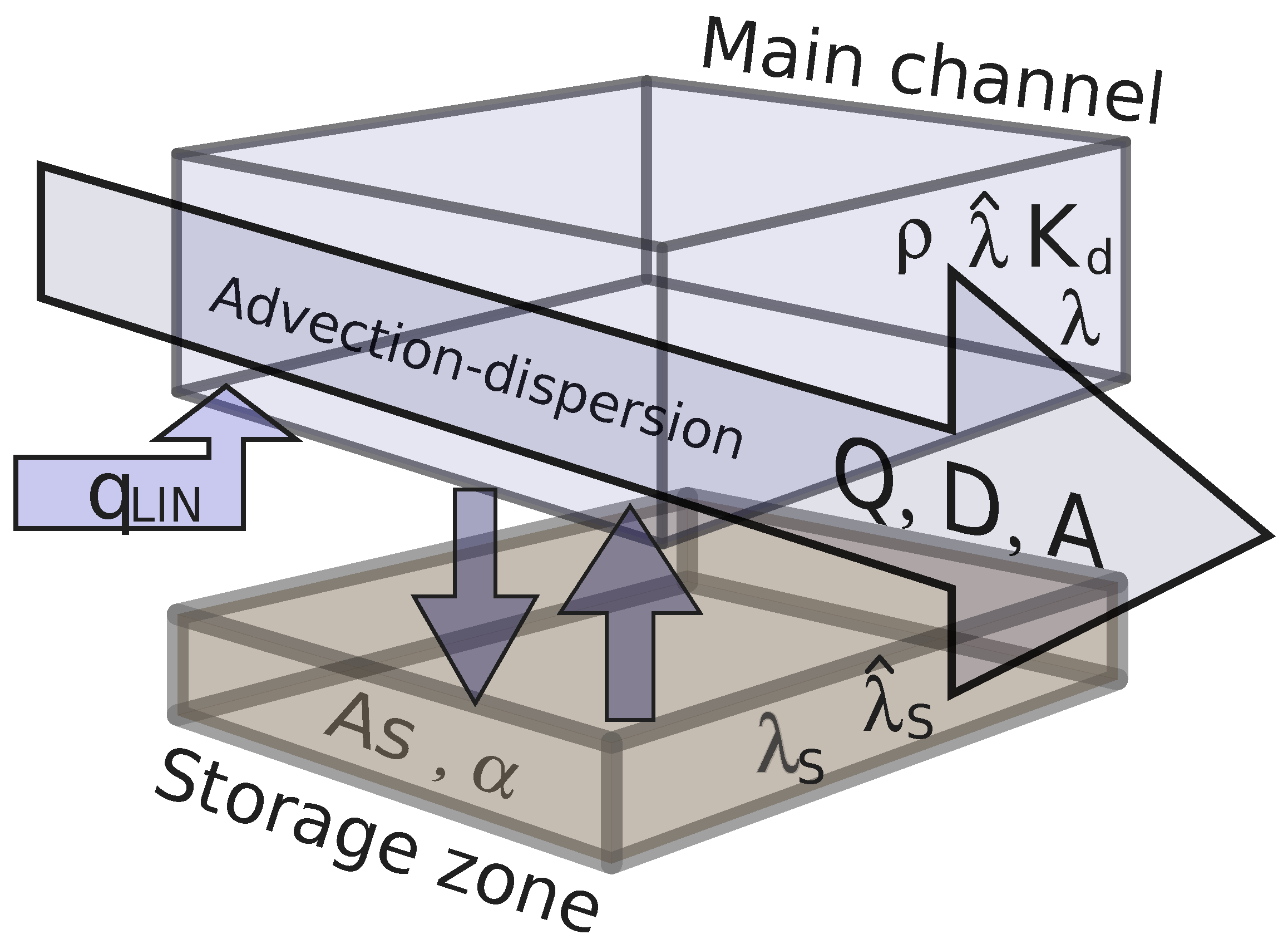
2.4. Data Treatment and Otis-P Modeling
3. Results and Discussion
3.1. Whole-Stretch Retention of Phosphorus
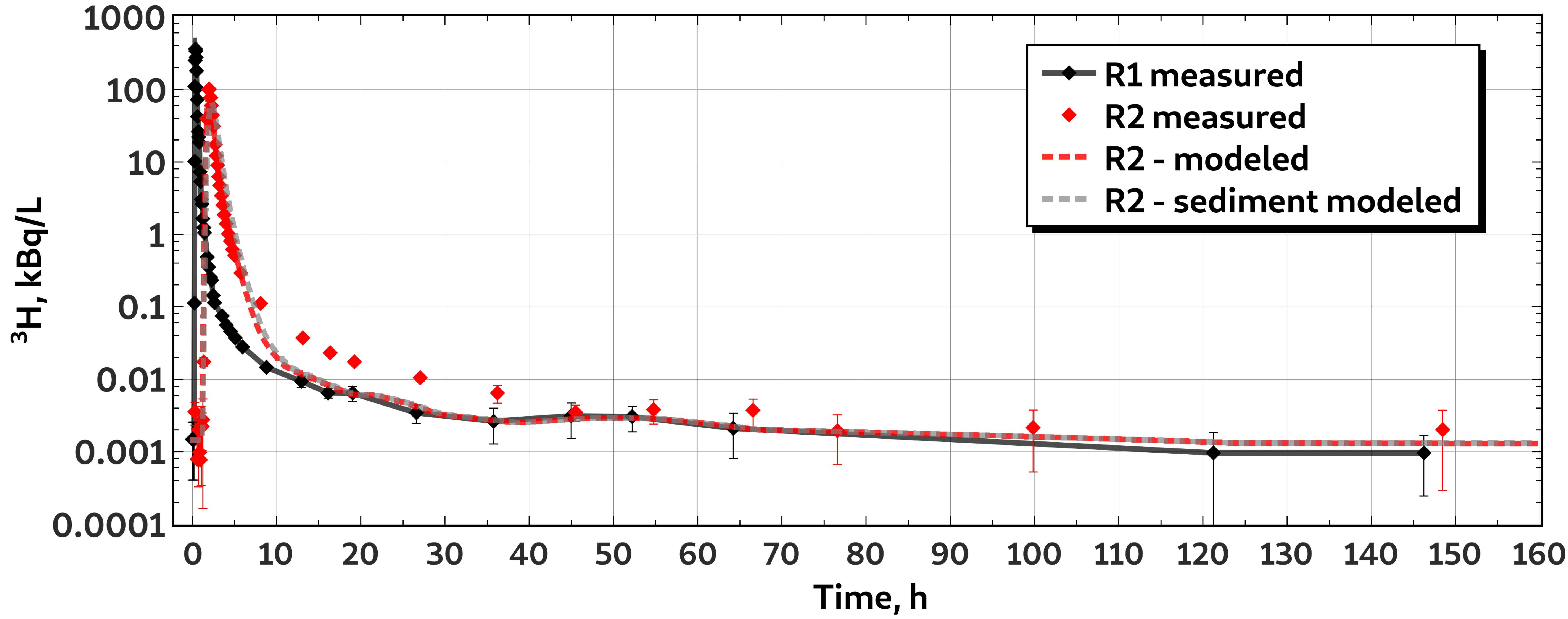
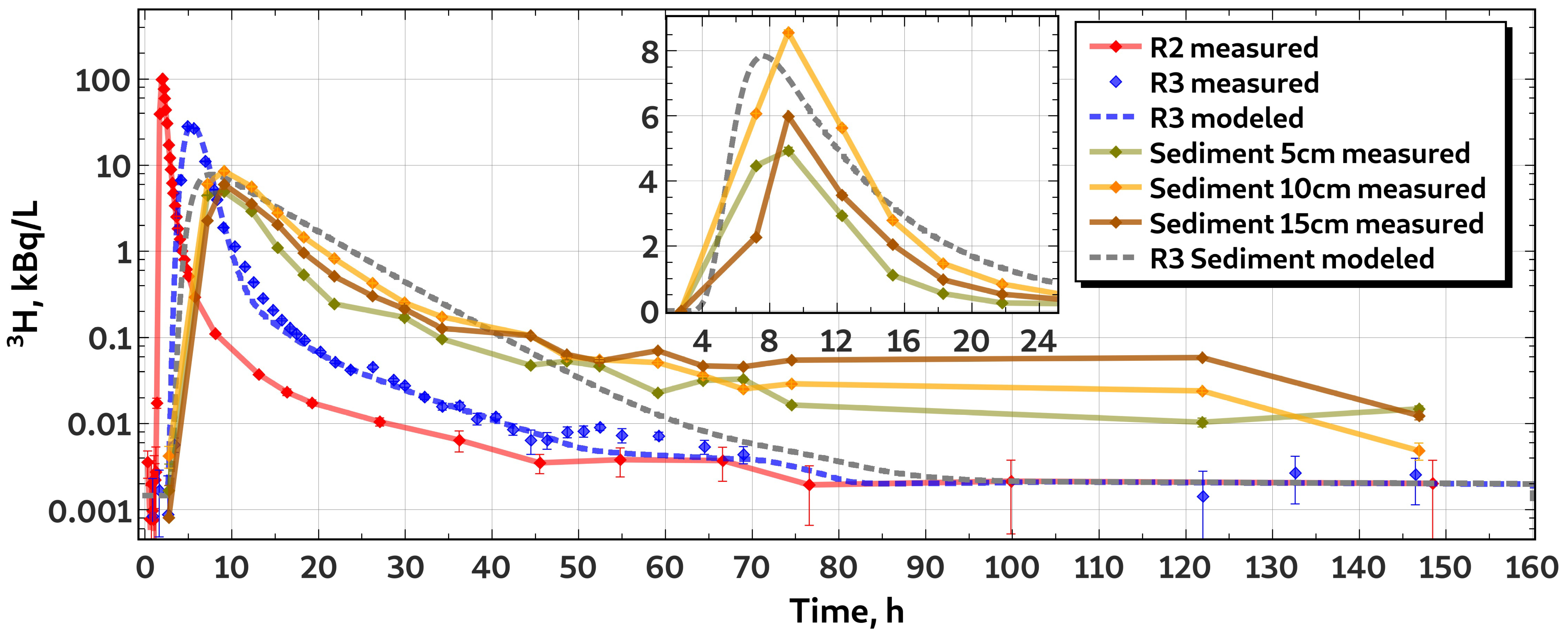
3.2. Characteristics of H Transport
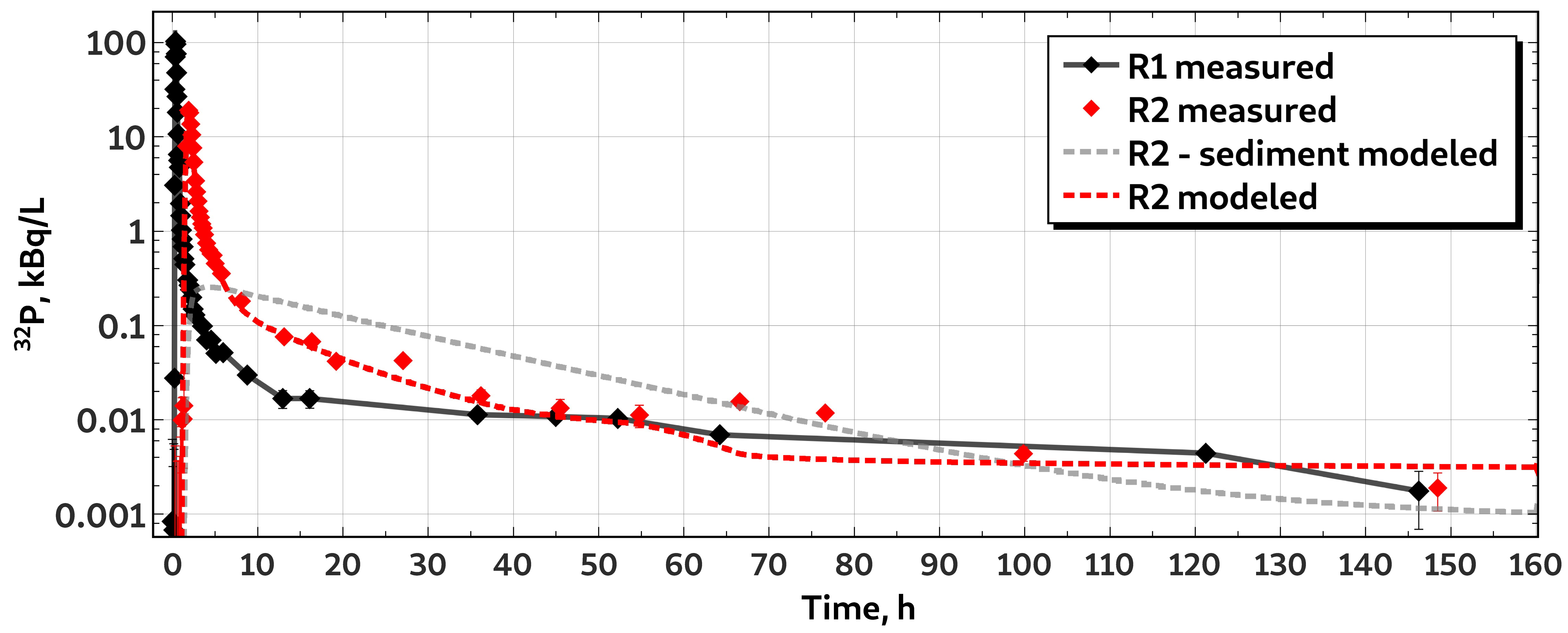
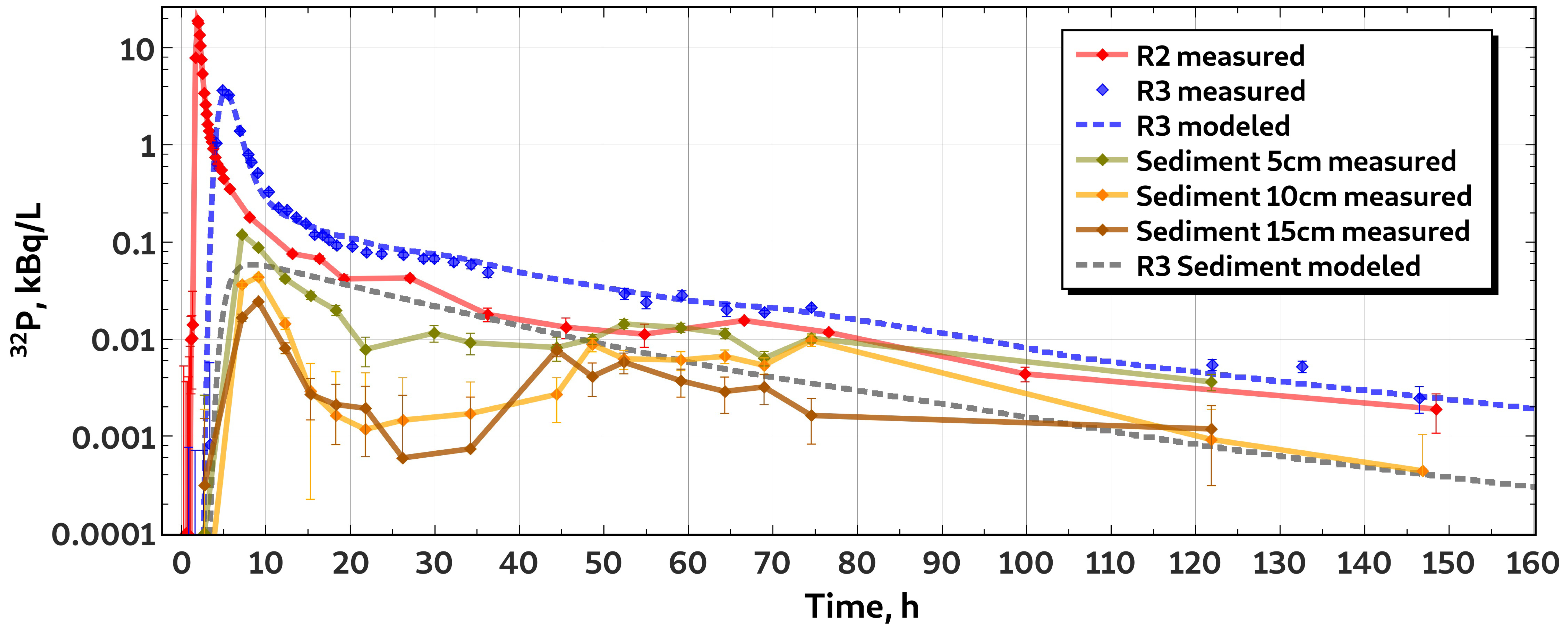
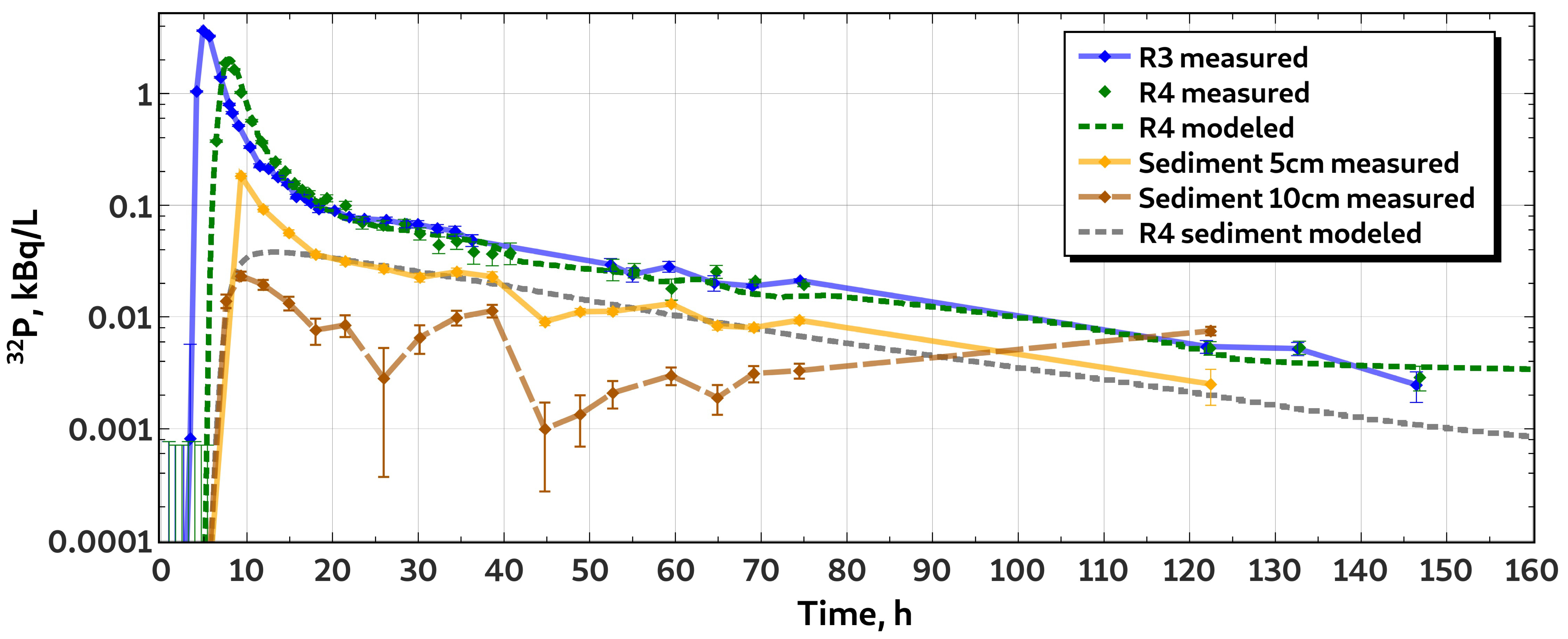
3.3. Characteristics of P Transport
4. Conclusions
Author Contributions
Funding
Institutional Review Board Statement
Informed Consent Statement
Data Availability Statement
Acknowledgments
Conflicts of Interest
Abbreviations
| BTC | Breakthrough curve |
| TDP | Total dissolved phosphorus |
Appendix A. In-Stream and Hyporheic Tracer Concentrations

| R1 | R2 | ||||
|---|---|---|---|---|---|
| Time [h] | c [kBq/L] | U(c) [kBq/L] | Time [h] | c [kBq/L] | U(c) [kBq/L] |
| 0.00 | 0.001 | 0.001 | 0.32 | 0.004 | 0.001 |
| 0.08 | 0.002 | 0.000 | 0.58 | 0.001 | 0.001 |
| 0.17 | 0.002 | 0.001 | 0.75 | 0.002 | 0.002 |
| 0.22 | 0.001 | 0.000 | 0.87 | 0.001 | 0.001 |
| 0.25 | 0.112 | 0.004 | 0.97 | 0.001 | 0.001 |
| 0.28 | 10.12 | 0.09 | 1.07 | 0.002 | 0.002 |
| 0.32 | 109.2 | 0.9 | 1.17 | 0.002 | 0.001 |
| 0.35 | 249.6 | 2.2 | 1.27 | 0.003 | 0.003 |
| 0.38 | 359.3 | 3.6 | 1.37 | 0.017 | 0.002 |
| 0.42 | 336.1 | 2.5 | 1.70 | 39.3 | 0.3 |
| 0.45 | 275.6 | 3.3 | 1.93 | 98.8 | 1.0 |
| 0.50 | 179.1 | 1.9 | 2.03 | 100.1 | 1.1 |
| 0.55 | 103.0 | 0.8 | 2.18 | 76.4 | 0.7 |
| 0.60 | 72.2 | 0.6 | 2.28 | 59.5 | 0.6 |
| 0.65 | 41.8 | 0.4 | 2.40 | 43.9 | 0.3 |
| 0.70 | 25.9 | 0.2 | 2.53 | 30.6 | 0.2 |
| 0.75 | 21.9 | 0.2 | 2.73 | 17.1 | 0.1 |
| 0.82 | 18.6 | 0.2 | 2.87 | 12.09 | 0.08 |
| 0.93 | 7.29 | 0.06 | 3.00 | 8.96 | 0.08 |
| 1.00 | 5.33 | 0.04 | 3.15 | 6.24 | 0.05 |
| 1.07 | 3.02 | 0.02 | 3.28 | 4.75 | 0.04 |
| 1.17 | 2.61 | 0.03 | 3.45 | 3.39 | 0.03 |
| 1.27 | 1.65 | 0.02 | 3.62 | 2.53 | 0.02 |
| 1.37 | 1.23 | 0.01 | 3.78 | 1.84 | 0.02 |
| 1.47 | 1.05 | 0.02 | 4.03 | 1.39 | 0.01 |
| 1.80 | 0.481 | 0.008 | 4.28 | 1.01 | 0.02 |
| 1.97 | 0.350 | 0.006 | 4.53 | 0.80 | 0.01 |
| 2.13 | 0.254 | 0.004 | 4.78 | 0.617 | 0.009 |
| 2.30 | 0.230 | 0.002 | 5.03 | 0.512 | 0.005 |
| 2.47 | 0.142 | 0.002 | 5.77 | 0.292 | 0.004 |
| 2.63 | 0.113 | 0.002 | 8.12 | 0.111 | 0.004 |
| 3.53 | 0.074 | 0.002 | 13.13 | 0.037 | 0.001 |
| 4.03 | 0.056 | 0.001 | 16.37 | 0.023 | 0.002 |
| 4.53 | 0.046 | 0.002 | 19.25 | 0.017 | 0.001 |
| 5.13 | 0.037 | 0.003 | 27.07 | 0.010 | 0.001 |
| 5.97 | 0.028 | 0.002 | 36.23 | 0.006 | 0.002 |
| 8.82 | 0.015 | 0.001 | 45.52 | 0.003 | 0.001 |
| 12.95 | 0.009 | 0.002 | 54.80 | 0.004 | 0.001 |
| 16.13 | 0.006 | 0.001 | 66.60 | 0.004 | 0.002 |
| 19.03 | 0.006 | 0.002 | 76.60 | 0.002 | 0.001 |
| 26.60 | 0.003 | 0.001 | 99.85 | 0.002 | 0.002 |
| 35.80 | 0.003 | 0.001 | 148.47 | 0.002 | 0.002 |
| 45.00 | 0.003 | 0.002 | |||
| 52.25 | 0.003 | 0.001 | |||
| 64.25 | 0.002 | 0.001 | |||
| 121.25 | 0.001 | 0.001 | |||
| 146.25 | 0.001 | 0.001 |
| R3 | R4 | ||||
|---|---|---|---|---|---|
| Time [h] | c [kBq/L] | U(c) [kBq/L] | Time [h] | c [kBq/L] | U(c) [kBq/L] |
| 0.90 | 0.001 | 0.001 | 0.95 | 0.001 | 0.002 |
| 1.65 | 0.002 | 0.001 | 1.70 | 0.002 | 0.003 |
| 2.65 | 0.001 | 0.002 | 2.45 | 0.002 | 0.003 |
| 3.40 | 0.006 | 0.001 | 3.20 | 0.002 | 0.002 |
| 4.15 | 6.7 | 0.1 | 3.95 | 0.001 | 0.002 |
| 4.90 | 28.0 | 0.2 | 4.70 | 0.002 | 0.001 |
| 5.62 | 26.7 | 0.2 | 5.42 | 0.002 | 0.003 |
| 6.93 | 11.0 | 0.1 | 6.45 | 3.49 | 0.02 |
| 7.95 | 5.18 | 0.05 | 7.48 | 19.9 | 0.1 |
| 8.30 | 3.99 | 0.03 | 8.50 | 16.9 | 0.1 |
| 9.05 | 1.88 | 0.01 | 9.32 | 10.3 | 0.1 |
| 10.37 | 1.13 | 0.01 | 10.57 | 4.35 | 0.03 |
| 11.52 | 0.660 | 0.008 | 11.75 | 1.944 | 0.013 |
| 12.52 | 0.434 | 0.007 | 13.32 | 0.867 | 0.007 |
| 13.62 | 0.283 | 0.005 | 14.47 | 0.523 | 0.006 |
| 14.75 | 0.207 | 0.004 | 15.55 | 0.350 | 0.005 |
| 15.78 | 0.159 | 0.004 | 16.47 | 0.260 | 0.004 |
| 16.72 | 0.128 | 0.003 | 17.28 | 0.206 | 0.005 |
| 17.48 | 0.110 | 0.002 | 18.57 | 0.146 | 0.004 |
| 18.40 | 0.093 | 0.003 | 19.33 | 0.123 | 0.003 |
| 20.23 | 0.068 | 0.002 | 21.52 | 0.083 | 0.002 |
| 21.93 | 0.052 | 0.002 | 23.47 | 0.064 | 0.004 |
| 23.70 | 0.042 | 0.002 | 25.90 | 0.047 | 0.002 |
| 26.27 | 0.045 | 0.003 | 28.40 | 0.044 | 0.002 |
| 28.65 | 0.032 | 0.001 | 30.20 | 0.038 | 0.003 |
| 29.95 | 0.028 | 0.001 | 32.40 | 0.031 | 0.002 |
| 32.23 | 0.020 | 0.001 | 34.50 | 0.022 | 0.002 |
| 34.28 | 0.016 | 0.002 | 36.48 | 0.016 | 0.002 |
| 36.28 | 0.016 | 0.002 | 38.65 | 0.015 | 0.002 |
| 38.30 | 0.011 | 0.002 | 40.75 | 0.013 | 0.001 |
| 40.43 | 0.012 | 0.001 | 42.65 | 0.013 | 0.002 |
| 42.43 | 0.009 | 0.001 | 44.80 | 0.012 | 0.001 |
| 44.50 | 0.006 | 0.002 | 46.75 | 0.009 | 0.002 |
| 46.37 | 0.006 | 0.001 | 48.92 | 0.011 | 0.001 |
| 48.70 | 0.008 | 0.001 | 50.75 | 0.010 | 0.001 |
| 50.58 | 0.008 | 0.001 | 52.72 | 0.009 | 0.001 |
| 52.45 | 0.009 | 0.001 | 55.22 | 0.010 | 0.001 |
| 55.00 | 0.007 | 0.001 | 59.55 | 0.007 | 0.001 |
| 59.25 | 0.007 | 0.001 | 64.78 | 0.006 | 0.001 |
| 64.52 | 0.005 | 0.001 | 69.30 | 0.004 | 0.001 |
| 69.00 | 0.004 | 0.001 | 75.00 | 0.004 | 0.001 |
| 74.57 | 0.008 | 0.001 | 122.40 | 0.003 | 0.001 |
| 121.98 | 0.001 | 0.001 | 132.83 | 0.003 | 0.001 |
| 132.62 | 0.003 | 0.001 | 146.87 | 0.001 | 0.001 |
| 146.48 | 0.003 | 0.001 |
| R3 (5 cm) | R3 (10 cm) | R3 (15 cm) | ||||
|---|---|---|---|---|---|---|
| Time [h] | c [kBq/L] | U(c) [kBq/L] | c [kBq/L] | U(c) [kBq/L] | c [kBq/L] | U(c) [kBq/L] |
| 2.75 | 0.002 | 0.002 | 0.004 | 0.001 | 0.001 | 0.001 |
| 7.20 | 4.46 | 0.05 | 6.07 | 0.08 | 2.27 | 0.03 |
| 9.12 | 4.92 | 0.10 | 8.56 | 0.07 | 5.99 | 0.08 |
| 12.30 | 2.93 | 0.07 | 5.63 | 0.05 | 3.56 | 0.04 |
| 15.30 | 1.10 | 0.01 | 2.79 | 0.03 | 2.04 | 0.04 |
| 18.30 | 0.532 | 0.008 | 1.46 | 0.03 | 0.958 | 0.009 |
| 21.80 | 0.244 | 0.004 | 0.825 | 0.007 | 0.512 | 0.005 |
| 26.22 | 0.67 | 0.01 | 0.424 | 0.009 | 0.303 | 0.005 |
| 29.92 | 0.170 | 0.003 | 0.252 | 0.003 | 0.213 | 0.004 |
| 34.22 | 0.096 | 0.003 | 0.173 | 0.003 | 0.127 | 0.002 |
| 44.43 | 0.047 | 0.002 | 0.105 | 0.002 | 0.105 | 0.002 |
| 48.63 | 0.053 | 0.002 | 0.059 | 0.002 | 0.063 | 0.002 |
| 52.38 | 0.046 | 0.002 | 0.055 | 0.002 | 0.053 | 0.002 |
| 59.13 | 0.023 | 0.002 | 0.051 | 0.001 | 0.070 | 0.002 |
| 64.32 | 0.032 | 0.002 | 0.036 | 0.001 | 0.047 | 0.001 |
| 68.97 | 0.033 | 0.002 | 0.025 | 0.001 | 0.046 | 0.002 |
| 74.55 | 0.016 | 0.001 | 0.029 | 0.001 | 0.054 | 0.002 |
| 121.88 | 0.010 | 0.001 | 0.024 | 0.001 | 0.058 | 0.002 |
| 146.88 | 0.015 | 0.001 | 0.005 | 0.001 | 0.012 | 0.001 |
| R4 (5 cm) | R4 (10 cm) | |||
|---|---|---|---|---|
| Time [h] | c [kBq/L] | U(c) [kBq/L] | c [kBq/L] | U(c) [kBq/L] |
| 3.00 | 0.002 | 0.001 | 0.001 | 0.001 |
| 5.00 | 0.005 | 0.001 | 0.001 | 0.001 |
| 7.58 | 6.1 | 0.1 | 0.281 | 0.002 |
| 9.33 | 12.0 | 0.1 | 1.72 | 0.01 |
| 11.92 | 6.03 | 0.07 | 4.31 | 0.04 |
| 14.92 | 2.28 | 0.02 | 4.77 | 0.02 |
| 18.03 | 0.748 | 0.008 | 2.64 | 0.02 |
| 21.48 | 0.279 | 0.003 | 1.67 | 0.01 |
| 25.98 | 0.111 | 0.002 | 1.099 | 0.008 |
| 30.18 | 0.067 | 0.002 | 0.792 | 0.005 |
| 34.48 | 0.041 | 0.001 | 0.464 | 0.004 |
| 38.65 | 0.022 | 0.002 | 0.315 | 0.002 |
| 44.78 | 0.020 | 0.001 | 0.160 | 0.001 |
| 48.90 | 0.019 | 0.001 | 0.151 | 0.001 |
| 52.70 | 0.013 | 0.001 | 0.135 | 0.001 |
| 59.52 | 0.009 | 0.001 | 0.063 | 0.001 |
| 64.92 | 0.028 | 0.001 | 0.078 | 0.001 |
| 69.15 | 0.035 | 0.001 | 0.076 | 0.001 |
| 74.48 | 0.024 | 0.001 | 0.075 | 0.001 |
| 122.48 | 0.033 | 0.002 | 0.175 | 0.002 |
| 146.48 | 0.007 | 0.001 | 0.119 | 0.001 |
| R1 | R2 | ||||
|---|---|---|---|---|---|
| Time [h] | c [kBq/L] | U(c) [kBq/L] | Time [h] | c [kBq/L] | U(c) [kBq/L] |
| 0.00 | <LOQ | - | 0.32 | <LOQ | - |
| 0.08 | <LOQ | - | 0.58 | <LOQ | - |
| 0.17 | <LOQ | - | 0.75 | <LOQ | - |
| 0.22 | <LOQ | - | 0.87 | <LOQ | - |
| 0.25 | 0.03 | 0.00 | 0.97 | <LOQ | - |
| 0.28 | 3.06 | 0.03 | 1.07 | <LOQ | - |
| 0.32 | 31.8 | 0.3 | 1.17 | 0.010 | 0.007 |
| 0.35 | 70.6 | 0.6 | 1.27 | 0.010 | 0.007 |
| 0.38 | 103.0 | 0.9 | 1.37 | 0.01 | 0.02 |
| 0.42 | 96.2 | 0.9 | 1.70 | 7.9 | 0.1 |
| 0.45 | 75.9 | 0.7 | 1.93 | 19.0 | 0.2 |
| 0.50 | 47.9 | 0.5 | 2.03 | 18.0 | 0.2 |
| 0.55 | 26.8 | 0.3 | 2.18 | 13.6 | 0.2 |
| 0.60 | 18.0 | 0.2 | 2.28 | 10.5 | 0.1 |
| 0.65 | 10.6 | 0.1 | 2.40 | 7.6 | 0.1 |
| 0.70 | 6.46 | 0.09 | 2.53 | 5.4 | 0.1 |
| 0.75 | 5.60 | 0.08 | 2.73 | 3.42 | 0.06 |
| 0.82 | 4.73 | 0.07 | 2.87 | 2.61 | 0.05 |
| 0.93 | 1.96 | 0.04 | 3.00 | 2.08 | 0.05 |
| 1.00 | 1.45 | 0.03 | 3.15 | 1.63 | 0.03 |
| 1.07 | 1.02 | 0.03 | 3.28 | 1.39 | 0.03 |
| 1.17 | 0.82 | 0.03 | 3.45 | 1.19 | 0.03 |
| 1.27 | 0.68 | 0.03 | 3.62 | 1.07 | 0.03 |
| 1.37 | 0.51 | 0.01 | 3.78 | 0.91 | 0.02 |
| 1.47 | 0.439 | 0.008 | 4.03 | 0.74 | 0.01 |
| 1.80 | 0.301 | 0.007 | 4.28 | 0.63 | 0.01 |
| 1.97 | 0.265 | 0.006 | 4.53 | 0.57 | 0.01 |
| 2.13 | 0.238 | 0.006 | 4.78 | 0.55 | 0.01 |
| 2.30 | 0.197 | 0.005 | 5.03 | 0.452 | 0.009 |
| 2.47 | 0.149 | 0.004 | 5.77 | 0.352 | 0.008 |
| 2.63 | 0.129 | 0.004 | 8.12 | 0.180 | 0.006 |
| 3.53 | 0.098 | 0.003 | 13.13 | 0.076 | 0.004 |
| 4.03 | 0.070 | 0.004 | 16.37 | 0.067 | 0.004 |
| 4.53 | 0.070 | 0.004 | 19.25 | 0.041 | 0.004 |
| 5.13 | 0.050 | 0.004 | 27.07 | 0.042 | 0.003 |
| 5.97 | 0.052 | 0.005 | 36.23 | 0.018 | 0.003 |
| 8.82 | 0.030 | 0.003 | 45.52 | 0.013 | 0.003 |
| 12.95 | 0.017 | 0.004 | 54.80 | 0.011 | 0.003 |
| 16.13 | 0.017 | 0.004 | 66.60 | 0.015 | 0.001 |
| 19.03 | 0.010 | 0.004 | 76.60 | 0.012 | 0.001 |
| 26.60 | 0.005 | 0.004 | 99.85 | 0.004 | 0.001 |
| 35.80 | 0.011 | 0.001 | 148.47 | 0.002 | 0.001 |
| 45.00 | 0.011 | 0.001 | |||
| 52.25 | 0.010 | 0.001 | |||
| 64.25 | 0.007 | 0.001 | |||
| 121.25 | 0.004 | 0.001 | |||
| 146.25 | 0.002 | 0.001 |
| R3 | R4 | ||||
|---|---|---|---|---|---|
| Time [h] | c [kBq/L] | U(c) [kBq/L] | Time [h] | c [kBq/L] | U(c) [kBq/L] |
| 0.90 | <LOQ | - | 0.95 | <LOQ | - |
| 1.65 | <LOQ | - | 1.70 | <LOQ | - |
| 2.65 | <LOQ | - | 2.45 | <LOQ | - |
| 3.4000 | 0.001 | 0.005 | 3.20 | <LOQ | - |
| 4.1500 | 1.04 | 0.02 | 3.95 | <LOQ | - |
| 4.9000 | 3.64 | 0.05 | 4.70 | <LOQ | - |
| 5.6167 | 3.26 | 0.05 | 5.42 | <LOQ | - |
| 6.9333 | 1.39 | 0.02 | 6.45 | 0.37 | 0.02 |
| 7.9500 | 0.80 | 0.02 | 7.48 | 1.87 | 0.02 |
| 8.3000 | 0.67 | 0.02 | 8.50 | 1.64 | 0.02 |
| 9.0500 | 0.51 | 0.01 | 9.32 | 1.02 | 0.01 |
| 10.3667 | 0.330 | 0.009 | 10.57 | 0.568 | 0.009 |
| 11.5167 | 0.225 | 0.009 | 11.75 | 0.364 | 0.009 |
| 12.5167 | 0.212 | 0.007 | 13.32 | 0.245 | 0.007 |
| 13.6167 | 0.178 | 0.005 | 14.47 | 0.200 | 0.005 |
| 14.7500 | 0.155 | 0.005 | 15.55 | 0.157 | 0.005 |
| 15.7833 | 0.119 | 0.006 | 16.47 | 0.137 | 0.006 |
| 16.7167 | 0.118 | 0.006 | 17.28 | 0.126 | 0.006 |
| 17.4833 | 0.105 | 0.006 | 18.57 | 0.103 | 0.006 |
| 18.4000 | 0.092 | 0.006 | 19.33 | 0.115 | 0.006 |
| 20.2333 | 0.089 | 0.004 | 21.52 | 0.100 | 0.004 |
| 21.9333 | 0.078 | 0.004 | 23.47 | 0.070 | 0.004 |
| 23.7000 | 0.075 | 0.004 | 25.90 | 0.066 | 0.004 |
| 26.2667 | 0.073 | 0.005 | 28.40 | 0.068 | 0.005 |
| 28.6500 | 0.067 | 0.005 | 30.20 | 0.056 | 0.005 |
| 29.9500 | 0.067 | 0.005 | 32.40 | 0.044 | 0.005 |
| 32.2333 | 0.062 | 0.005 | 34.50 | 0.048 | 0.005 |
| 34.2833 | 0.059 | 0.006 | 36.48 | 0.038 | 0.006 |
| 36.2833 | 0.048 | 0.006 | 38.65 | 0.037 | 0.006 |
| 38.3000 | 0.034 | 0.006 | 40.75 | 0.038 | 0.006 |
| 52.4500 | 0.029 | 0.004 | 42.65 | 0.013 | 0.005 |
| 55.0000 | 0.024 | 0.003 | 44.80 | 0.020 | 0.005 |
| 59.2500 | 0.028 | 0.003 | 46.75 | 0.009 | 0.005 |
| 64.5167 | 0.020 | 0.003 | 48.92 | 0.026 | 0.009 |
| 69.0000 | 0.019 | 0.001 | 50.75 | 0.027 | 0.006 |
| 74.5667 | 0.021 | 0.001 | 52.72 | 0.027 | 0.010 |
| 121.9833 | 0.005 | 0.001 | 55.22 | 0.026 | 0.004 |
| 132.6167 | 0.005 | 0.001 | 59.55 | 0.018 | 0.003 |
| 146.4833 | 0.002 | 0.001 | 64.78 | 0.025 | 0.003 |
| 69.30 | 0.021 | 0.003 | |||
| 75.00 | 0.019 | 0.001 | |||
| 122.40 | 0.005 | 0.001 | |||
| 132.83 | 0.005 | 0.001 | |||
| 146.87 | 0.003 | 0.001 |
| R3 (5 cm) | R3 (10 cm) | R3 (15 cm) | ||||
|---|---|---|---|---|---|---|
| Time [h] | c [kBq/L] | U(c) [kBq/L] | c [kBq/L] | U(c) [kBq/L] | c [kBq/L] | U(c) [kBq/L] |
| 2.75 | <LOQ | - | <LOQ | - | <LOQ | - |
| 7.20 | 0.119 | 0.003 | 0.036 | 0.002 | 0.017 | 0.001 |
| 9.12 | 0.088 | 0.003 | 0.044 | 0.002 | 0.024 | 0.001 |
| 12.30 | 0.042 | 0.002 | 0.014 | 0.002 | 0.008 | 0.001 |
| 15.30 | 0.028 | 0.002 | 0.003 | 0.003 | 0.003 | 0.001 |
| 18.30 | 0.020 | 0.002 | 0.002 | 0.003 | 0.002 | 0.001 |
| 21.80 | 0.008 | 0.003 | 0.001 | 0.003 | 0.002 | 0.001 |
| 26.22 | 0.012 | 0.002 | 0.001 | 0.003 | 0.001 | 0.002 |
| 29.92 | 0.009 | 0.002 | <LOQ | - | <LOQ | - |
| 34.22 | 0.008 | 0.002 | 0.002 | 0.002 | 0.001 | 0.002 |
| 44.43 | 0.010 | 0.001 | 0.003 | 0.001 | 0.008 | 0.001 |
| 48.63 | 0.014 | 0.001 | 0.009 | 0.001 | 0.004 | 0.002 |
| 52.38 | 0.013 | 0.001 | 0.006 | 0.001 | 0.006 | 0.001 |
| 59.13 | 0.011 | 0.001 | 0.006 | 0.001 | 0.004 | 0.001 |
| 64.32 | 0.006 | 0.001 | 0.007 | 0.001 | 0.003 | 0.001 |
| 68.97 | 0.010 | 0.001 | 0.005 | 0.001 | 0.003 | 0.001 |
| 74.55 | 0.004 | 0.001 | <LOQ | - | 0.002 | 0.001 |
| 121.88 | <LOQ | - | 0.010 | 0.001 | 0.001 | 0.001 |
| 146.88 | <LOQ | - | 0.001 | 0.001 | <LOQ | - |
| R4 (5 cm) | R4 (10 cm) | |||
|---|---|---|---|---|
| Time [h] | c [kBq/L] | U(c) [kBq/L] | c [kBq/L] | U(c) [kBq/L] |
| 3.00 | <LOQ | - | <LOQ | - |
| 5.00 | <LOQ | - | 0.011 | 0.002 |
| 7.58 | 0.140 | 0.008 | 0.014 | 0.002 |
| 9.33 | 0.182 | 0.010 | 0.023 | 0.002 |
| 11.92 | 0.092 | 0.005 | 0.019 | 0.002 |
| 14.92 | 0.056 | 0.003 | 0.013 | 0.002 |
| 18.03 | 0.036 | 0.003 | 0.008 | 0.002 |
| 21.48 | 0.031 | 0.002 | 0.008 | 0.002 |
| 25.98 | 0.027 | 0.002 | 0.003 | 0.002 |
| 30.18 | 0.022 | 0.002 | 0.007 | 0.002 |
| 34.48 | 0.025 | 0.002 | 0.010 | 0.001 |
| 38.65 | 0.023 | 0.002 | 0.011 | 0.001 |
| 44.78 | 0.009 | 0.001 | 0.001 | 0.001 |
| 48.90 | 0.011 | 0.001 | 0.001 | 0.001 |
| 52.70 | 0.011 | 0.001 | 0.002 | 0.001 |
| 59.52 | 0.013 | 0.001 | 0.003 | 0.001 |
| 64.92 | 0.008 | 0.001 | 0.002 | 0.001 |
| 69.15 | 0.008 | 0.001 | 0.003 | 0.001 |
| 74.48 | 0.009 | 0.001 | 0.003 | 0.001 |
| 122.48 | 0.003 | 0.001 | 0.007 | 0.001 |
| 146.48 | <LOQ | - | <LOQ | - |
Appendix B

Appendix C. List of Symbols
| C | main channel solute concentration |
| lateral inflow solute concentration | |
| storage zone solute concentration | |
| L | reach length |
| A | main channel cross-section area |
| Q | volumetric flow rate (discharge) |
| u | mean water velocity |
| D | dispersion coefficient |
| storage zone exchange coefficient | |
| storage zone cross-section area | |
| main channel first-order decay coefficient | |
| storage zone first-order decay coefficient | |
| main channel sorption rate coefficient | |
| storage zone sorption rate coefficient | |
| distribution coefficient | |
| mass of accesible sediment/volume water | |
| dispersion parameter | |
| storage zone depth | |
| average distance a molecule travels downstream within the main channel prior to entering the storage zone | |
| the main channel residence time | |
| is the storage zone residence time | |
| storage exchange flux | |
| hydrological retention factor | |
| mean travel time due to the main channel | |
| mean travel time due to storage zone | |
| mean travel time | |
| fraction of median travel time due to transient storage |
References
- Jarvie, H.P.; Sharpley, A.N.; Scott, J.T.; Haggard, B.E.; Bowes, M.J.; Massey, L.B. Within-river phosphorus retention: Accounting for a missing piece in the watershed phosphorus puzzle. Environ. Sci. Technol. 2012, 46, 13284–13292. [Google Scholar] [CrossRef] [PubMed] [Green Version]
- Jarvie, H.P.; Sharpley, A.N.; Withers, P.J.; Scott, J.T.; Haggard, B.E.; Neal, C. Phosphorus mitigation to control river eutrophication: Murky waters, inconvenient truths, and “postnormal” science. J. Environ. Qual. 2013, 42, 295–304. [Google Scholar] [CrossRef] [PubMed]
- Withers, P.; Jarvie, H. Delivery and cycling of phosphorus in rivers: A review. Sci. Total Environ. 2008, 400, 379–395. [Google Scholar] [CrossRef]
- Haggard, B.E.; Sharpley, A.N.; Radcliffe, D.; Cabrera, M. Phosphorus transport in streams: Processes and modeling considerations. In Modeling Phosphorus in the Environment; CRC Press: Boca Raton, FL, USA, 2006; pp. 105–130. [Google Scholar]
- Mainstone, C.P.; Parr, W. Phosphorus in rivers—Ecology and management. Sci. Total Environ. 2002, 282, 25–47. [Google Scholar] [CrossRef]
- Doyle, M.W.; Stanley, E.H.; Harbor, J.M. Hydrogeomorphic controls on phosphorus retention in streams. Water Resour. Res. 2003, 39. [Google Scholar] [CrossRef] [Green Version]
- Newbold, J.; Elwood, J.; O’neill, R.; Sheldon, A. Phosphorus dynamics in a woodland stream ecosystem: A study of nutrient spiralling. Ecology 1983, 64, 1249–1265. [Google Scholar] [CrossRef]
- Newbold, J.D.; Elwood, J.W.; O’Neill, R.V.; Winkle, W.V. Measuring nutrient spiralling in streams. Can. J. Fish. Aquat. Sci. 1981, 38, 860–863. [Google Scholar] [CrossRef]
- Webster, J.R.; Patten, B.C. Effects of watershed perturbation on stream potassium and calcium dynamics. Ecol. Monogr. 1979, 49, 51–72. [Google Scholar] [CrossRef] [Green Version]
- Barbieri, M. Isotopes in Hydrology and Hydrogeology. Water 2019, 11, 291. [Google Scholar] [CrossRef] [Green Version]
- Leibundgut, C.; Maloszewski, P.; Kulls, C. Tracers in Hydrology; John Wiley & Sons: Chichester, UK, 2011. [Google Scholar]
- Wörman, A.; Wachniew, P. Reach scale and evaluation methods as limitations for transient storage properties in streams and rivers. Water Resour. Res. 2007, 43. [Google Scholar] [CrossRef]
- Małoszewski, P.; Wachniew, P.; Czupryński, P. Hydraulic Characteristics of a Wastewater Treatment Pond Evaluated through Tracer Test and Multi-Flow Mathematical Approach. Pol. J. Environ. Stud. 2006, 15, 105–110. [Google Scholar]
- Małoszewski, P.; Wachniew, P.; Czupryński, P. Study of hydraulic parameters in heterogeneous gravel beds: Constructed wetland in Nowa Słupia (Poland). J. Hydrol. 2006, 331, 630–642. [Google Scholar] [CrossRef]
- Mulholland, P.J.; Steinman, A.D.; Elwood, J.W. Measurement of phosphorus uptake length in streams: Comparison of radiotracer and stable PO4 releases. Can. J. Fish. Aquat. Sci. 1990, 47, 2351–2357. [Google Scholar] [CrossRef]
- Stutter, M.; Demars, B.; Langan, S. River phosphorus cycling: Separating biotic and abiotic uptake during short-term changes in sewage effluent loading. Water Res. 2010, 44, 4425–4436. [Google Scholar] [CrossRef] [PubMed]
- Lal, D.; Malhotra, P.; Peters, B. On the production of radioisotopes in the atmosphere by cosmic radiation and their application to meteorology. J. Atmos. Terr. Phys. 1958, 12, 306–328. [Google Scholar] [CrossRef]
- Lal, D.; Narasappaya, N.; Zutshi, P.K. Phosphorus isotopes P-32 and P-33 in rain water. Nucl. Phys. 1957, 3, 69–75. [Google Scholar] [CrossRef]
- Gupta, A.; Destouni, G.; Jensen, M.B. Modelling Subsurface Phosphorus Transport; Groundwater in the Urban Environment-Vol I: Problems, Processes and Management; A Balkema: Leiden, The Netherlands, 1997; pp. 417–420. [Google Scholar]
- Nagy, N.M.; Buzetzky, D.; Kovacs, E.M.; Kovacs, A.B.; Katai, J.; Vago, I.; Jozsef, K. Study of phosphate species of chernozem and sand soils by heterogeneous isotope exchange with P-32 radioactive tracer. Appl. Radiat. Isot. 2019, 152, 64–71. [Google Scholar] [CrossRef]
- Spohn, M.; Zavišić, A.; Nassal, P.; Bergkemper, F.; Schulz, S.; Marhan, S.; Schloter, M.; Kandeler, E.; Polle, A. Temporal variations of phosphorus uptake by soil microbial biomass and young beech trees in two forest soils with contrasting phosphorus stocks. Soil Biol. Biochem. 2018, 117, 191–202. [Google Scholar] [CrossRef] [Green Version]
- Hayes, F.; McCarter, J.; Cameron, M.; Livingstone, A.D. On the kinetics of phosphorus exchange in lakes. J. Ecol. 1952, 40, 202–216. [Google Scholar] [CrossRef]
- Rigler, F. A tracer study of the phosphorus cycle in lake water. Ecology 1956, 37, 550–562. [Google Scholar] [CrossRef]
- Ball, R.; Hooper, F. Translocation of Phosphorus in a Trout Stream Ecosystem, Progress Report, June 14, 1961 to March 7, 1962; Department of Fisheries and Wildlife, Michigan State University: East Lansing, MI, USA, 1962. [Google Scholar]
- Garder, K.; Skulberg, O. Experimental Investigation on the Accumulation of Radioisotopes by Fresh Water Biota; Institute for Atomic Energy: Kjeller, Norway, 1966. [Google Scholar]
- Nelson, D.; Kevern, N.; Wilhm, J.; Griffith, N. Estimates of periphyton mass and stream bottom area using phosphorous-32. Water Res. 1969, 3, 367–373. [Google Scholar] [CrossRef]
- Elwood, J.W.; Nelson, D.J. Periphyton production and grazing rates in a stream measured with a 32 P material balance method. Oikos 1972, 23, 295–303. [Google Scholar] [CrossRef]
- Mulholland, P.J.; Newbold, J.D.; Elwood, J.W.; Ferren, L.A.; Webster, J.R. Phosphorus spiralling in a woodland stream: Seasonal variations. Ecology 1985, 66, 1012–1023. [Google Scholar] [CrossRef] [Green Version]
- Walker, I.; Henderson, P.A.; Sterry, P. On the patterns of biomass transfer in the benthic fauna of an Amazonian black-water river, as evidenced by 32 P label experiment. Hydrobiologia 1991, 215, 153–162. [Google Scholar] [CrossRef]
- Mulholland, P.J.; Marzolf, E.R.; Webster, J.R.; Hart, D.R.; Hendricks, S.P. Evidence that hyporheic zones increase heterotrophic metabolism and phosphorus uptake in forest streams. Limnol. Oceanogr. 1997, 42, 443–451. [Google Scholar] [CrossRef]
- Payn, R.A.; Webster, J.R.; Mulholland, P.J.; Valett, H.M.; Dodds, W.K. Estimation of stream nutrient uptake from nutrient addition experiments. Limnol. Oceanogr. Methods 2005, 3, 174–182. [Google Scholar] [CrossRef] [Green Version]
- Gooddy, D.C.; Lapworth, D.J.; Bennett, S.A.; Heaton, T.H.; Williams, P.J.; Surridge, B.W. A multi-stable isotope framework to understand eutrophication in aquatic ecosystems. Water Res. 2016, 88, 623–633. [Google Scholar] [CrossRef] [Green Version]
- Paytan, A.; McLaughlin, K. Tracing the sources and biogeochemical cycling of phosphorus in aquatic systems using isotopes of oxygen in phosphate. In Handbook of Environmental Isotope Geochemistry; Springer: Berlin/Heidelberg, Germany, 2012; pp. 419–436. [Google Scholar]
- Pistocchi, C.; Tamburini, F.; Gruau, G.; Ferhi, A.; Trevisan, D.; Dorioz, J.M. Tracing the sources and cycling of phosphorus in river sediments using oxygen isotopes: Methodological adaptations and first results from a case study in France. Water Res. 2017, 111, 346–356. [Google Scholar] [CrossRef] [PubMed] [Green Version]
- Withers, P.; Jarvie, H.; Stoate, C. Quantifying the impact of septic tank systems on eutrophication risk in rural headwaters. Environ. Int. 2011, 37, 644–653. [Google Scholar] [CrossRef]
- Withers, P.; Jarvie, H.; Hodgkinson, R.; Palmer-Felgate, E.; Bates, A.; Neal, M.; Howells, R.; Withers, C.; Wickham, H. Characterization of phosphorus sources in rural watersheds. J. Environ. Qual. 2009, 38, 1998–2011. [Google Scholar] [CrossRef]
- Piasecki, A. Water and sewage management issues in rural Poland. Water 2019, 11, 625. [Google Scholar] [CrossRef] [Green Version]
- Acuña, V.; Casellas, M.; Font, C.; Romero, F.; Sabater, S. Nutrient attenuation dynamics in effluent dominated watercourses. Water Res. 2019, 160, 330–338. [Google Scholar] [CrossRef]
- Painter, K.J.; Brua, R.B.; Spoelstra, J.; Koehler, G.; Yates, A.G. Fate of bioavailable nutrients released to a stream during episodic effluent releases from a municipal wastewater treatment lagoon. Environ. Sci. Process. Impacts 2020, 22, 2374–2387. [Google Scholar] [CrossRef]
- Waiser, M.J.; Tumber, V.; Holm, J. Effluent-dominated streams. Part 1: Presence and effects of excess nitrogen and phosphorus in Wascana Creek, Saskatchewan, Canada. Environ. Toxicol. Chem. 2011, 30, 496–507. [Google Scholar] [CrossRef]
- Powers, S.M.; Stanley, E.H.; Lottig, N.R. Quantifying phosphorus uptake using pulse and steady-state approaches in streams. Limnol. Oceanogr. Methods 2009, 7, 498–508. [Google Scholar] [CrossRef] [Green Version]
- Gooseff, M.N.; Payn, R.A.; Zarnetske, J.P.; Bowden, W.B.; McNamara, J.P.; Bradford, J.H. Comparison of in-channel mobile–immobile zone exchange during instantaneous and constant rate stream tracer additions: Implications for design and interpretation of non-conservative tracer experiments. J. Hydrol. 2008, 357, 112–124. [Google Scholar] [CrossRef]
- Payn, R.A.; Gooseff, M.N.; Benson, D.A.; Cirpka, O.A.; Zarnetske, J.P.; Bowden, W.B.; McNamara, J.P.; Bradford, J.H. Comparison of instantaneous and constant-rate stream tracer experiments through non-parametric analysis of residence time distributions. Water Resour. Res. 2008, 44. [Google Scholar] [CrossRef] [Green Version]
- Runkel, R.L. One-Dimensional Transport with Inflow and Storage (OTIS): A Solute Transport Model for Streams and Rivers; U.S. Department of the Interior; U.S. Geological Survey: Hunter Mill, VA, USA, 1998; Volume 98.
- Van Metre, P.C.; Waite, I.R.; Qi, S.; Mahler, B.; Terando, A.; Wieczorek, M.; Meador, M.; Bradley, P.; Journey, C.; Schmidt, T.; et al. Projected urban growth in the southeastern USA puts small streams at risk. PLoS ONE 2019, 14, e0222714. [Google Scholar] [CrossRef] [PubMed]
- Brazier, R.E.; Puttock, A.; Graham, H.A.; Auster, R.E.; Davies, K.H.; Brown, C.M. Beaver: Nature’s ecosystem engineers. Wiley Interdiscip. Rev. Water 2021, 8, e1494. [Google Scholar] [CrossRef]
- Wróbel, M. Population of Eurasian beaver (Castor fiber) in Europe. Glob. Ecol. Conserv. 2020, 23, e01046. [Google Scholar] [CrossRef]
- Olesen, J.E.; Børgesen, C.D.; Hashemi, F.; Jabloun, M.; Bar-Michalczyk, D.; Wachniew, P.; Zurek, A.J.; Bartosova, A.; Bosshard, T.; Hansen, A.L. Nitrate leaching losses from two Baltic Sea catchments under scenarios of changes in land use, land management and climate. Ambio 2019, 48, 1252–1263. [Google Scholar] [CrossRef]
- Refsgaard, J.C.; Hansen, A.L.; Højberg, A.L.; Olesen, J.E.; Hashemi, F.; Wachniew, P.; Wörman, A.; Bartosova, A.; Stelljes, N.; Chubarenko, B. Spatially differentiated regulation: Can it save the Baltic Sea from excessive N-loads? Ambio 2019, 48, 1278–1289. [Google Scholar] [CrossRef]
- Zięba, D.; Michalczyk, T.; Bar-Michalczyk, D.; Jaszczur, M.; Żurek, A.; Wachniew, P. Identification of groundwater contribution to streamflow in a medium-size catchment. Przegląd Geol. 2015, 63, 1161–1165. (In Polish) [Google Scholar]
- Barsby, A. Determination of mixing lengths in dilution gauging. In Proceedings of the Symposium on Geochemistry, Precipitation, Evaporation, Soil-Moisture, Hydrometry, General Assembly of Bern, Bern, Switzerland, 25 September–7 October 1967; International Association of Scientific Hydrology: Wallingford, UK, 1967; pp. 395–407. [Google Scholar]
- Florkowski, T. Tritium in river flow-rate gauging-theory and experience. In Use of Artificial Tracers in Hydrology; IAEA: Vienna, Austria, 1991; pp. 35–44. [Google Scholar]
- Harvey, J.; Wagner, B. The Physical Template: Hydrology, Hydraulics, and Physical Structure; Stream and Ground Waters Academic Press: New York, NY, USA, 2000; pp. 3–44. [Google Scholar]
- Jarvie, H.P.; Withers, J.; Neal, C. Review of robust measurement of phosphorus in river water: Sampling, storage, fractionation and sensitivity. Hydrol. Earth Syst. Sci. 2002, 6, 113–131. [Google Scholar] [CrossRef] [Green Version]
- Baken, S.; Regelink, I.C.; Comans, R.N.; Smolders, E.; Koopmans, G.F. Iron-rich colloids as carriers of phosphorus in streams: A field-flow fractionation study. Water Res. 2016, 99, 83–90. [Google Scholar] [CrossRef] [PubMed]
- River, M.; Richardson, C.J. Stream transport of iron and phosphorus by authigenic nanoparticles in the Southern Piedmont of the US. Water Res. 2018, 130, 312–321. [Google Scholar] [CrossRef] [PubMed]
- Wagner, B.J.; Gorelick, S.M. A statistical methodology for estimating transport parameters: Theory and applications to one-dimensional advectivec-dispersive systems. Water Resour. Res. 1986, 22, 1303–1315. [Google Scholar] [CrossRef]
- Workshop, S.S. Concepts and methods for assessing solute dynamics in stream ecosystems. J. N. Am. Benthol. Soc. 1990, 9, 95–119. [Google Scholar] [CrossRef]
- Puttock, A.; Graham, H.A.; Cunliffe, A.M.; Elliott, M.; Brazier, R.E. Eurasian beaver activity increases water storage, attenuates flow and mitigates diffuse pollution from intensively-managed grasslands. Sci. Total Environ. 2017, 576, 430–443. [Google Scholar] [CrossRef] [Green Version]
- Bohrman, K.J.; Strauss, E.A. Macrophyte-driven transient storage and phosphorus uptake in a western Wisconsin stream. Hydrol. Process. 2018, 32, 253–263. [Google Scholar] [CrossRef]
- Valett, H.M.; Crenshaw, C.L.; Wagner, P.F. Stream nutrient uptake, forest succession, and biogeochemical theory. Ecology 2002, 83, 2888–2901. [Google Scholar] [CrossRef]
- Niyogi, D.K.; Simon, K.S.; Townsend, C.R. Land use and stream ecosystem functioning: Nutrient uptake in streams that contrast in agricultural development. Arch. Fur. Hydrobiol. 2004, 160, 471–486. [Google Scholar] [CrossRef]
- Gottselig, N.; Bol, R.; Nischwitz, V.; Vereecken, H.; Amelung, W.; Klumpp, E. Distribution of phosphorus-containing fine colloids and nanoparticles in stream water of a forest catchment. Vadose Zone J. 2014, 13, 1–11. [Google Scholar] [CrossRef]
- Boano, F.; Harvey, J.W.; Marion, A.; Packman, A.I.; Revelli, R.; Ridolfi, L.; Wörman, A. Hyporheic flow and transport processes: Mechanisms, models, and biogeochemical implications. Rev. Geophys. 2014, 52, 603–679. [Google Scholar] [CrossRef]
- Knapp, J.L.; Kelleher, C. A perspective on the future of transient storage modeling: Let’s stop chasing our tails. Water Resour. Res. 2020, 56, e2019WR026257. [Google Scholar] [CrossRef] [Green Version]
- Runkel, R.L. A new metric for determining the importance of transient storage. J. N. Am. Benthol. Soc. 2002, 21, 529–543. [Google Scholar] [CrossRef] [Green Version]
- Femeena, P.; Chaubey, I.; Aubeneau, A.; McMillan, S.; Wagner, P.; Fohrer, N. Simple regression models can act as calibration-substitute to approximate transient storage parameters in streams. Adv. Water Resour. 2019, 123, 201–209. [Google Scholar] [CrossRef]


| Point | 5 April | 7 April |
|---|---|---|
| R1 | 0.142 | 0.095 |
| R2 | - | - |
| R3 | - | 0.111 |
| R4 | 0.202 | 0.147 |
| Point | Distance [m] | Recovered P [GBq] | Recovered H [GBq] | P/H | P Recovery Relative to R1 | P Retention Relative to R1 |
|---|---|---|---|---|---|---|
| R1 | 305 | 10.86 | 37.3 | 0.29 | 1 | 0 |
| R2 | 970 | 8.84 | 37.9 | 0.23 | 0.80 | 0.20 |
| R3 | 1540 | 6.74 | 37.5 | 0.18 | 0.62 | 0.38 |
| R4 | 2594 | 5.98 | 37.9 | 0.16 | 0.54 | 0.46 |
| Stretch | v [m/s] | W [m] | Q [m/s] | [m] | [1/s] | [mm/min] |
|---|---|---|---|---|---|---|
| Velocity | Width | Discharge | Uptake Length | Uptake Coeff. | Uptake Velocity | |
| R1–R2 | 0.116 | 3.5 | 0.132 | 2931 | 3.6 × 10 | 0.75 |
| R2–R3 | 0.049 | 4.7 | 0.133 | 2225 | 1.8 × 10 | 0.78 |
| R3–R4 | 0.152 | 3.5 | 0.166 | 8130 | 1.5 × 10 | 0.35 |
| R1-R4 | 0.094 | 3.9 | 0.166 | 3736 | 2.1 × 10 | 0.68 |
| Parameter/Metric | Unit | R1–R2 | R2–R3 | R3–R4 |
|---|---|---|---|---|
| L | [m] | 665 | 570 | 1054 |
| A | [m ] | 1.23 | 3.18 | 1.30 |
| Q | [m/s] | 0.132 | 0.133 | 0.166 |
| [m/s] | 0.107 | 0.042 | 0.127 | |
| D | [m/s] | 0.989 | 0.882 | 0.850 |
| [1/s] | 4.61 × 10 | 1.11 × 10 | 8.94 × 10 | |
| [m ] | 0.098 | 0.120 | 0.074 | |
| [-] | 0.074 | 0.036 | 0.054 | |
| [-] | 0.014 | 0.037 | 0.006 | |
| [m] | 0.049 | 0.030 | 0.037 | |
| [m] | 2.51 × 10 | 4.37 × 10 | 1.70 × 10 | |
| [h] | 4.8 | 9.5 | 17.7 | |
| [h] | 60 | 250 | 311 | |
| [m/s] | 5.66 × 10 | 3.53 × 10 | 1.17 × 10 | |
| [s/m] | 0.691 | 0.778 | 0.376 | |
| [h] | 1.64 | 3.47 | 1.95 | |
| [h] | 0.16 | 0.42 | 0.14 | |
| [h] | 1.80 | 3.89 | 2.10 | |
| F | 6.33 × 10 | 1.91 × 10 | 7.56 × 10 |
| Parameter/Metric | Unit | R1–R2 | R2–R3 | R3–R4 |
|---|---|---|---|---|
| L | [m] | 665 | 570 | 1054 |
| A | [m ] | 1.213 | 3.22 | 1.40 |
| Q | [m/s] | 0.132 | 0.133 | 0.166 |
| [m/s] | 0.109 | 0.041 | 0.119 | |
| D | [m/s] | 0.926 | 0.900 | 0.830 |
| 8.76 × 10 | 9.27 × 10 | 9.40 × 10 | ||
| [m ] | 0.423 | 1.350 | 0.674 | |
| [1/s] | 1.92 × 10 | 2.44 × 10 | 1.02 × 10 | |
| [1/s] | 2.13 × 10 | 1.83 × 10 | 1.03 × 10 | |
| [1/s] | 2.87 × 10 | 1.27 × 10 | 1.28 × 10 | |
| [1/s] | 2.50 × 10 | 2.50 × 10 | 2.50 × 10 | |
| [m/kg] | 200.000 | 200.000 | 200.000 | |
| [kg/m] | 8.98 × 10 | 7.90 × 10 | 4.14 × 10 | |
| [-] | 0.259 | 0.295 | 0.325 | |
| [-] | 0.012 | 0.033 | 0.006 | |
| [m] | 0.212 | 0.338 | 0.169 | |
| [m] | 1.34 × 10 | 5.17 × 10 | 1.50 × 10 | |
| [h] | 4.8 | 9.5 | 17.7 | |
| [h] | 32 | 300 | 296 | |
| [m/s] | 1.06 × 10 | 2.98 × 10 | 1.32 × 10 | |
| R = T/L | [s/m] | 0.691 | 0.778 | 0.376 |
| t = Lu + 2D/u | [h] | 1.62 | 3.52 | 2.10 |
| t = (A/A) × t | [h] | 0.68 | 4.75 | 1.41 |
| t = t + t | [h] | 2.30 | 8.27 | 3.51 |
| F | [-] | 4.13 × 10 | 1.31 × 10 | 4.93 × 10 |
Publisher’s Note: MDPI stays neutral with regard to jurisdictional claims in published maps and institutional affiliations. |
© 2021 by the authors. Licensee MDPI, Basel, Switzerland. This article is an open access article distributed under the terms and conditions of the Creative Commons Attribution (CC BY) license (https://creativecommons.org/licenses/by/4.0/).
Share and Cite
Zięba, D.; Wachniew, P. Phosphorus Transport in a Lowland Stream Derived from a Tracer Test with 32P. Water 2021, 13, 1030. https://doi.org/10.3390/w13081030
Zięba D, Wachniew P. Phosphorus Transport in a Lowland Stream Derived from a Tracer Test with 32P. Water. 2021; 13(8):1030. https://doi.org/10.3390/w13081030
Chicago/Turabian StyleZięba, Damian, and Przemysław Wachniew. 2021. "Phosphorus Transport in a Lowland Stream Derived from a Tracer Test with 32P" Water 13, no. 8: 1030. https://doi.org/10.3390/w13081030