Abstract
Water quality prediction plays a crucial role in both enterprise management and government environmental management. However, due to the variety in water quality data, inconsistent frequency of data acquisition, inconsistency in data organization, and volatility and sparsity of data, predicting water quality accurately and efficiently has become a key problem. This paper presents a recurrent neural network water quality prediction method based on a sequence-to-sequence (seq2seq) framework. The gate recurrent unit (GRU) model is used as an encoder and decoder, and a factorization machine (FM) is integrated into the model to solve the problem of high sparsity and high dimensional feature interaction in the data, which was not addressed by the water quality prediction models in prior research. Moreover, due to the long period and timespan of water quality data, we add a dual attention mechanism to the seq2seq framework to address memory failures in deep learning. We conducted a series of experiments, and the results show that our proposed method is more accurate than several typical water quality prediction methods.
1. Introduction
The protection of water resources is an extremely important aspect of sustainable development of natural environments, and water pollution has become one of the most urgent problems in the world. However, in recent years, with the increasing technological advancement of industry and the increasing number of factories, improper treatment of waste materials and wastewater in some factories is the most significant cause of water pollution in various regions. When regional water quality integrity is corrupted by pollution, the living environment of the surrounding biosphere is also seriously threatened, which eventually endangers the ecology of entire water areas [1,2]. Therefore, the governance of water environments has become increasingly important, and, in this field, the prediction of water quality data plays a pivotal role. If the pollution sources can be directed to handle hazardous material appropriately before contamination occurs, water quality treatment could become significantly easier [3]. However, prediction of water quality data faces many challenges, including the following: (1) There are many indicators included in water quality data. According to the regulations of the National Environmental Protection Department, basic pollutants include 24 indicators, and various chemical elements and organic compounds, which together account for a total of 109 different indicators. The greater the number of indicators, the higher the requirements for parallel computing on the predictive model. (2) The sampling frequency of water quality data is not fixed. Because different monitoring indicators have different chemical attributes, the monitoring stations sample different monitoring indicators at different frequencies, for hourly, daily, and monthly monitoring. The diversification of sampling frequency contributes varying degrees of increased difficulty in data processing and model construction. (3) The indicators of water quality data are not independent of each other. There are hundreds of indicators for water quality data, but different indicators are not necessarily independent of each other and may have complex correlations such as deep causality. If the relationship between the indexes cannot be accurately extracted, the accuracy of a water quality prediction model is greatly reduced. (4) The time span of water quality data is very long. Since environmental governance is not a short-term task, it takes years to process and protect water quality, which results in a very long time span for water quality monitoring data, and interpretative models of water quality monitoring data from many years ago still have an impact on the prediction of future water quality, which becomes a critical issue in model construction. Due to the above-mentioned challenges, traditional water quality prediction models often use basic linear models, such as logistic regression [4]. However, because the linear regression model does not consider the nonlinear relationship between the characteristics of water quality data and are prone to large errors in cases of unbalanced data, it is often impossible to obtain highly accurate prediction values. In response to the above-mentioned problems, this paper proposes a new time series forecasting model called FM-GRU, by integrating a factorization machine with the seq2seq framework, thereby leveraging their combined advantages. By applying dual attention to time steps and covariates, our proposed model can obtain accurate time series prediction results. The main contributions of this paper are as follows:
(1) We apply the method of factorization machines to time series forecasting. High-dimensional feature information in the time series is extracted for covariable prediction, solving the complicated and time-consuming problems of traditional artificial feature engineering.
(2) We add a dual attention mechanism to the traditional seq2seq framework, solving the problem of decoding distraction and long-range information loss.
(3) We input the high-dimensional features obtained in the FM into the improved encoder–decoder model to co-train the FM model and the improved encoder–decoder model and make prediction. Our experimental results show that our FM-GRU model is better than seven advanced time series prediction methods on water quality data from Lianjiang River in Guangdong, China.
The remainder of this article is organized as follows: Section 2 introduces related work and background information; Section 3 elaborates on the principle and structure of our proposed FM-GRU model and describes the corresponding algorithm; Section 4 introduces the experimental procedure and results. Finally, Section 5 summarizes the article and discusses directions for future research.
2. Related Work
In recent years, the field of water quality prediction has received increasing attention. In response to the above-mentioned problems and the shortcomings of traditional water quality models, scholars have proposed many efficient algorithms and models.
2.1. Statistics and Machine Learning Methods
For the water quality prediction problem, prior statistical or traditional machine learning methods generally focus on autoregressive single-step prediction. Such algorithms often fail to achieve excellent results in multi-step prediction. Jaynes [5] proposed the classic autoregressive integrated moving average model (ARIMA) model, which uses the autoregressive method of difference and moving average to predict time series. Cardoso and Cruz [6] proposed a time series analysis model integrating ARIMA and an artificial neural network (ANN). Although ARIMA cannot extract interaction between nonlinear features, the ANN neural network makes up for this shortcoming, and thus the experimental results are much better than those for traditional ARIMA. Li et al. [7] combined a support vector machine (SVM) with chaos theory and calculated the delay and embedding dimension parameters of a phase space reconstruction based on mutual information and the false nearest neighbor method. The accuracy of this model was demonstrated on the Lorentz chaotic time series. Behzad et al. [8] analyzed the reservoir flow data of the Bakhtiari Dam, demonstrating that, under the condition of an optimal parameter selection, SVM has a higher prediction accuracy than the classic ANN and ANN-genetic algorithms (ANN-GA). Shiri et al. [9] used extreme learning machines (ELM) to predict the water level sequence data of Urima Lake, and their results show that ELM has better performance than genetic programming (GP) and ANN, and the training time of GP is much lower than that of traditional feedforward neural networks, whereas accuracy is almost unaffected. Yang et al. [10] used the water level data provided by the Shimen Reservoir monitoring station in Taiwan as a dataset and performed water level prediction using a time series analysis model based on a random forest algorithm. Experiments show that, when data are complete, the random forest approach has a higher prediction accuracy than the traditional statistical model. Guo et al. [11] improved the SVM to a least squares support vector machine (LSSVM). This improved model enhances the prediction accuracy of SVM in most cases and has therefore been applied to daily water level forecasting of the Yangtze River. However, traditional statistical methods usually cannot obtain many potential feature relationships. Moreover, machine learning solutions often require complex feature work in early stages. Therefore, it becomes necessary to find critical features before training, which requires a large amount of practical experience and domain-specific knowledge of scholars to manually realize, and this becomes the bottleneck of machine learning in terms of data analysis.
2.2. Deep Learning Methods
In addition to traditional statistics and machine learning methods, in recent years, with the enhancement of computational power as well as the rapid development of central processing units (CPUs) and graphics processing units (GPUs), deep learning began to be noted for performing well on time series analysis, gradually surpassing and replacing traditional machine learning in time series forecasting. Xiao and Si [12] proposed a time series analysis model they called a long short-term memory and dynamic Bayesian network (LSTM-DBN) by combining long short-term memory (LSTM) and Bayesian graph inference. Through the best estimation principle and recursive algorithm training parameters, the accuracy of LSTM was improved. Winata et al. [13] introduced an attention mechanism in an encoder–decoder model, aiming to design a model that devoted more attention resources to certain target regions of a time series to simulate the internal process of natural cognitive observation. In this attention mechanism, the model applies greater weight parameters to the more important timing components in the encoder to improve the model’s accuracy. The mentioned study further demonstrates that bidirectional LSTM (BiLSTM) has a higher accuracy in time series analysis than the one-way LSTM. Ye et al. [14] proposed the application of a recurrent neural network (RNN) variant, using an LSTM model to analyze Shanghai river water quality monitoring data, demonstrating the ability to extract information from earlier data in predicting a long-time-span water quality data sequence. Dong et al. [15] proposed a model called SG-ED-LSTM. The model uses an encoder–decoder framework embedded in an LSTM cell to achieve multi-step prediction. In the data preprocessing stage, the Savitzky–Golay (SG) filter was used to filter the original data. This method can improve the smoothness of the time series and reduce noise interference while maintaining the shape and length of the time series. Tang et al. [16] proposed a novel approach using variational modal decomposition (VMD) to decompose complex wind speed time series into more simplified models, combined with GRU to predict the wind speed interval. This provided a new direction for data processing methods in time series analysis. Barzegar et al. [17] proposed a state-of-the-art method to combine a convolutional neural network (CNN) with LSTM. This hybrid CNN-LSTM model takes water quality data sequences as input for a convolutional layer structure to perform feature extraction and then passes them through the flattening layer as input of the LSTM architecture to obtain the predicted value of the target. After experimental comparison, this solution integrates the advantages of the two classic models of CNN and RNN. The CNN layer is used to understand the sequential features of the input, while the lower LSTM layer integrates these functions by processing the remote dependencies of the predicted target value. Pan et al. [18] proposed a CNN-GRU model to predict the water level of the Yangtze River. GRU reduces the number of gates on the basis of LSTM, that is, it reduces the number of parameters, which can greatly reduce the operation time without affecting accuracy, which is more efficient than the LSTM [19]. The disadvantage of the above two schemes is that CNNs are very sensitive to sparse data, and datasets in real world applications are often not perfect, while various null or singular values are prone to appear, which may significantly affect the ability of a CNN to obtain feature information. Wang et al. [20] proposed a model called DC-LSTM, which adopts a model architecture integrating dilated convolution and LSTM. Experiments prove that the dilated convolution method has higher accuracy than the original CNN on chaotic time series.
2.3. Preliminaries
Linear regression models [21] and logistic regression models have played an important role in regression and prediction problems in the past decades. They are relatively simple linear models, focusing on capturing the linear relationship between features. The principle is clear and easy to understand. The training speed is considered satisfactory; hence, linear regression models are commonly used to provide simple solutions to general regression and prediction problems. However, the shortcomings of the linear model are also obvious. In the real world, features are often not independent of each other but have potential internal connections, such as male consumers’ preference for sports products and female consumers’ preference for beauty products, and these internal connections can neither be captured in a linear model nor fit the nonlinear relationship between features. However, these potential nonlinear relationships between features are highly meaningful to the performance of such models. Therefore, several scholars have considered artificially adding nonlinear relations to improve performance, that is, adding artificial feature engineering to logistic regression [22]. This method became widely used as soon as it was proposed, and it still plays an important role in the modern industry. However, this model has an obvious disadvantage, that is, artificial feature combination is a very time-consuming and laborious work. Because of the various types and the large amounts of feature data available in industries, it is very difficult to accurately capture these nonlinear feature combinations manually; therefore, it often takes a considerable amount of human resources to perform this work, which is not conducive to industrial cost control. In addition, artificial feature engineering based on experience may not be able to capture hidden laws in the feature data, resulting in a decrease in model performance.
Rendle [23] proposed a factorization machine (FM) approach in 2010, solving two problems: (1) Because FM can obtain interactive relationships between different index data, FM shows better performance on sparse datasets. (2) FM solves the defect that traditional logistic regression can only obtain linear feature information and cannot capture nonlinear features (especially cross-feature information). This makes it possible to extract high-dimensional features from training data in Click-Through-Rate research [24,25] or service quality research [26]. Moreover, the training time complexity of FM is linear and efficient, solving the cumbersome problem of artificial feature engineering. Because the fluctuation of water quality indicators is affected by a variety of complex factors, this study uses FM in the feature extraction of water quality time series data to obtain potential relationships between water quality features. Then, the output of the FM model is input to the encoder GRU in our improved seq2seq framework.
seq2seq is a deep learning framework first proposed by the Google Brain team Vaswani et al. [27] to solve time series analysis problems such as machine translation. There exists in the literature no good solution to the problem of machine translation because traditional time series prediction models such as recurrent neural networks (RNNs) and variants cannot freely determine the length of input and output sequences, whereas, in actual practice, the input and output sequences often differ in length. The core purpose of the seq2seq framework is to solve this bottleneck using encoding and decoding methods. The information of the input sequence is encoded into a fixed-size semantic vector using an encoder, and an output sequence is obtained from the decoder. In the field of machine translation, the words and sentences to be translated are often short, to avoid loss of long-range information. However, in the water quality time series prediction problem in this study, owing to the particularity of water quality data, the time span of the data may be as long as several years. The amount of data we will deal with will be much larger than the amount of data in the translation problem, which will bring a serious long-range information loss problem. In short, the data from a long time ago will have minimal impact on the encoded semantic vector, but the previous data still have important significance for prediction, and the loss of this information is unacceptable to us. Therefore, we have added a dual attention mechanism to the traditional seq2seq framework, in addition to using the traditional attention mechanism to apply varying weights to time steps, adding attention to covariates. In this way, the influence of different covariates on the target are obtained, so as to enhance the model’s predictive ability for time series with a larger span, and at the same time make the model more scalable.
3. Model Framework
3.1. Overall Framework
Our model aims to solve the problem of predicting a next time sequence when one component of time sequence is known. To this end, we propose a model called the FM-GRU. Figure 1 shows the overall framework of the model, including the relationship between the FM module and the improved seq2seq module as well as the flow of training and verification data. to are the covariate inputs in the encoding stage, to are the covariate inputs in the decoding stage, and to are the predicted values corresponding to the decoding stage. The following is a detailed description of the implementation of each module and the construction of the overall model framework:
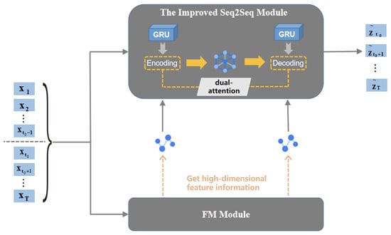
Figure 1.
FM-GRU model framework.
3.2. FM Module
In this part, our goal is to obtain high-dimensional feature information of time series data by establishing an FM model, as shown in Figure 2, we build an FM model that contains bias, linear terms, and high-dimensional nonlinear terms:
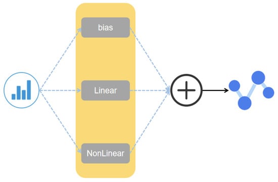
Figure 2.
FM model.
The expression of FM model can be expressed in Equation (1):
where represents the bias, represents the parameter of , and represents the parameter of the cross term . The number of parameters in this model is 1 + n + n(n − 1)/2, which are independent of each other between any two parameters of the high-order combination feature. This will cause a serious problem in practical applications, since the data obtained in real life are often not perfect, some of the data are often missing, and the cross term is very sensitive to the missing data, which will cause the parameters to be unable to train normally, and the performance of this model in the real dataset will be seriously affected. Therefore, FM introduces the idea of matrix decomposition, models the parameters of the cross term, and introduces the auxiliary matrix V to estimate. The cross term after decomposition is , thereinto
Thus, we can get the :
Substituting (3) into the cross term in (1), we get:
where the < , > means dot product.
Note that the auxiliary matrix V contains a hyperparameter K that needs to be defined by ourselves, which will affect the performance of the model to some extent. Obviously, the time complexity of the cross term of the above model is , but through mathematical methods, the above model can be optimized into the following formula:
Now, we can get the simplified FM model expression:
The time complexity of the optimized model is .
3.3. The Improved seq2seq Framework
The model constructed by the traditional seq2seq framework has good prediction performance for time series data and can freely set the known time step and the predicted time step. However, for long-term time series, there are two situations where long-range information is lost:
(1) Data information with an earlier time step during encoding is far from the semantic vector (cell state) at the end of the sentence, and their information is easy to lose in the semantic vector.
(2) If the preset time step during decoding is long, the covariate data information in the initial decoding stage is likely to be lost after multiple time steps.
This easily lost long-range information is still very important, so we have added dual-Attention to the improved seq2seq framework. By applying different weights to the output of each time step of the encoding stage and applying different weights to each covariate x of the decoding stage, the dual attention to the time step and the covariate is realized.
As shown in Figure 3, the left part is the coding part. For encoder h, we use the GRU [28,29] model. Its expression is:
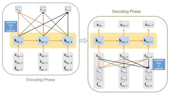
Figure 3.
Dual-Attention in the improved seq2seq module.
The input of each time step is the hidden layer h of the previous time step and the known target value z, the covariate x of the current time step and the output f of the FM model, represents the output of the GRU model at time step , and represents the hidden layer at time step . The GRU model is a recurrent autoregressive neural network, which can reduce the parameters of the model while achieving the same performance as the LSTM model, thereby reducing the running time of the model.
Figure 4 shows the basic external input and output structure of GRU. We have made some improvements to it, the output vector of the FM model at this time step and the target value at the previous moment and the covariate x are simultaneously input into the GRU model, and the neural network width of the GRU model is adjusted accordingly.
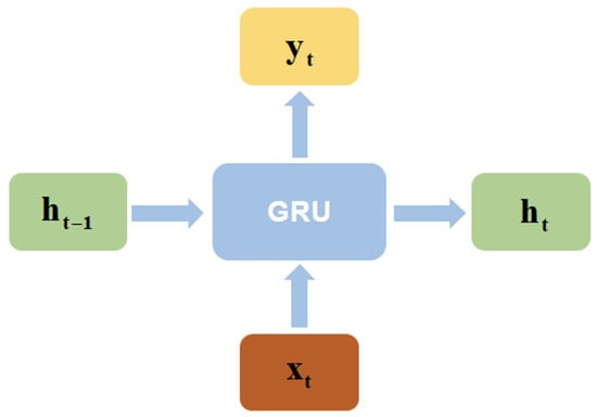
Figure 4.
The external input and output structure of the GRU model.
The right part of Figure 3 is the decoding part, the input of each time step is the covariate x of the current time step, the output f of the FM model, and the two parts of the vector about attention, which are the attention given to the output of the training stage and the attention given to the input covariate x of the decoding stage that is:
To maintain consistency, we still use the GRU model as the decoder.
Figure 5 shows how to obtain dual-Attention in the improved seq2seq model, this figure takes three time steps in the entire decoding process as an example and uses as the current time step to describe the implementation of dual-Attention in detail.
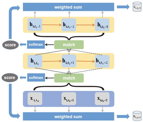
Figure 5.
Acquisition of dual-Attention.
The calculation steps of dual-Attention are as follows:
(1) At the time step , take the hidden state h of the time step to match all the covariates x in the decoding phase and the output of the last layer of all time steps in the encoding phase. There are many options for the ways to match, such as using the cos() function or building a neural network. The method used in this model is to first perform a linear transformation on the two tensors to be matched, and then use the two tensors as a matrix multiplication.
(2) Perform normalized exponential function (we use softmax( ) function) on the result of matrix multiplication to obtain two score results.
(3) Use the scores as the weight to do a weighted summation of all covariates x and all outputs of the encoding stage, so that we get and , and these two will then be used as input to the model at the time step .
Another difference from the coding stage is that the output y of the decoding stage will be used to measure the error of the model so that the parameters can be trained or the model can be evaluated. Here, we do not use the output y of each time step of the decoding stage for the next model input, the reason is that this will cause serious error accumulation problems in actual situations.
3.4. FM-GRU
From the above two sections, we can get the implementation principle of the FM module and the improved seq2seq model. From the perspective of the overall framework, the collaborative training process of the two provides the FM module with high-order feature information of covariates to the improved seq2seq during the encoding and decoding stages. seq2seq uses the GRU model as the encoder and decoder to achieve the efficiency and stability of the model, the dual-Attention acquired in the decoding process inputs the acquired long-range information into the decoder, and finally the decoder outputs the prediction results corresponding to decode_step steps.
In detail, the overall prediction process of the model can be divided into three steps. The first step is the encoding process. Encoding the covariate x and label to be input so that the dimension is the same as the hyperparameter hidden_size of the model and input the encoded covariate x into the FM model to obtain the multi-dimensional feature information f of x, then input this multi-dimensional feature information f, covariate x, label, and hidden state of the last time step into the GRU model, repeat the above process until the end of the encoding step. The second step is the decoding process. First, obtain the output f of the FM model (i.e., multi-dimensional feature information) in the same way, then obtain the Attention of different time steps of decoding through the covariate x of the decoding stage and the output of the encoding stage, and obtain two attention vectors by weighting and summing them respectively. They are input into the GRU decoder together with the covariate x, multi-dimensional feature information f, and the hidden state to obtain the output predicted value. At this time, use the GRU output and the actual target to perform error analysis and parameter adjustment, and repeat the training epochs times. Finally, the model is used to predict the value of the future time step in the same way.
Algorithm 1 summarizes the principles and steps of the FM-GRU model, shown by pseudo code. In Algorithm 1, history_x represents the covariates of the encoding stage, history_z represents the labels of the encoding stage, future_x represents the covariates of the decoding stage, hidden_attn represents the attention given to the time step, and hidden_x represents the attention given to the covariate.
| Algorithm 1 TSF using FM-GRU |
| Input: A multivariate time series R(N*T), encode_step, decode_step, K and all the other model parameters. Output:
|
Note that the other parameters mentioned above include hidden_size, num_layers, K, epochs, batch_size, learning rate, and drop_rate. In the specific implementation, we will enter a fixed value in each parameter.
4. Experiment
The main content of this section is divided into the following three parts: (1) Introduction to the dataset used in the experimental part; (2) Comparison and summary of the results obtained in the experiment with other time series models; (3) Discussion of three key parameter variables that affect the performance of this model: K, batch_size, learning_rate.
4.1. Dataset Description
The dataset we use is a variety of national water quality reference index data monitored by Haimen Bay monitoring station (https://www.shantou.gov.cn/epd/) (accessed on 8 April 2021) in Lianjiang River, Shantou City, China from 1 January 2019 to 30 June 2020. The Haimen Bay Monitoring Station belongs to the main stream monitoring station of the Lianjiang River and is at 23 degrees 2189 min latitude and 116 degrees 6189 min longitude. Figure 6 shows the geographic location of the Haimen Bay Monitoring Station. Since the Haimen Bay Monitoring Station is located at the estuary of the Lianjiang River, it is very important to monitor the overall water quality of the Lianjiang River; therefore, the state has designated the Haimen Bay monitoring station as a state-controlled monitoring station. At present, the Haimen Bay Monitoring Station monitors a total of 24 indicators. Among them, the ones that are of great significance to the treatment of water pollution are: dissolved oxygen, PH, conductivity, turbidity, total nitrogen, total phosphorus, sulfide, cyanide, volatile phenol, potassium permanganate index, etc. According to the surface water environmental quality standards promulgated by the state (GB 3838-2002) and the water quality data monitored by the monitoring station, the water quality assessment result of Lianjiang River in 2020 is inferior to the Class V standard, which is a seriously polluted water area that needs urgent treatment. Due to the different characteristics of different water quality indicators, the monitoring stations have different monitoring frequencies for different indicators. It is obvious that using data with different monitoring frequencies will affect the performance of the model. Therefore, we selected five water quality indicators with the same monitoring frequency (all one hour) from this dataset: water temperature, pH, conductivity, turbidity, and dissolved oxygen. The dissolved oxygen was used as the target for prediction, and the remaining four indicators were used as covariates.
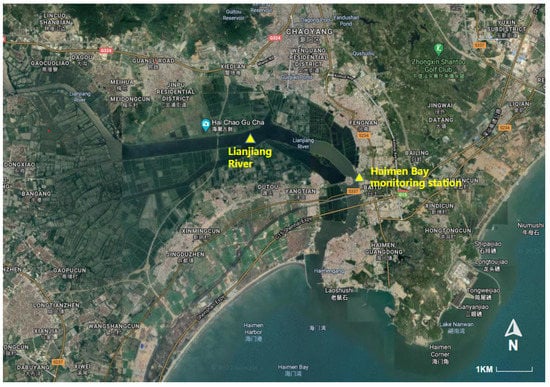
Figure 6.
The geographical location of the Haimen Bay Monitoring Station.
Figure 7 is the data display of the four covariate data in the first 100 time steps in this dataset (for the convenience of display, the data in the figure have been normalized). The dataset we have is very large. It contains 13,128 h of data, and the time span is up to one and a half years. Therefore, we take out a subset of 1000 time points in chronological order as the dataset for our experiment, that is, the size of this dataset is (1000*5). Table 1 is a brief summary of water quality data, showing some common mathematical characteristics of the data, including MAX (maximum), MIN (minimum), Mean (mean value), Median, Mode, SD (standard deviation).
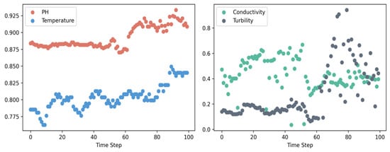
Figure 7.
Example time series of dataset.

Table 1.
Several characteristics of water quality data.
4.2. Data Preprocessing
The Lianjiang River Basin is the third largest river basin in eastern Guangdong, with a total length of 71.1 km and a drainage area of 1353 square kilometers. There are more than 20 tributaries, more than 40 monitoring stations, and more than 20 monitoring indicators. Due to the wide basin and different regional characteristics, the monitoring of the river section by the monitoring points will be affected by many factors such as weather, seasons, monitoring equipment, and man-made factors. Therefore, we have some null values in the Lianjiang River water quality monitoring dataset. Since the FM model in the FM-GRU model proposed in this paper has a strong ability to process sparse matrices, this experiment does not process the null values in the input covariates, only the label in the dataset, that is, dissolved oxygen is linearly filled. In addition, due to the different levels of water quality indicators, for example, the value of electrical conductivity may be thousands of times the PH value, we normalize and standardize the data of all indicators to avoid insufficient parameter training and data deviation problems of low-level indicators due to the magnitude of the data. Here, we use the traditional normalization method to map the water quality data to a decimal between 0–1, so as to avoid insufficient training of model parameters due to different data levels. At the same time, we use Z-score standardization to change the distribution of the original messy data to meet the normal distribution with a mean of 1 and a variance of 0, which will speed up the convergence of the model. The following formulas are the normalization and standardization calculation methods we use, Formula (9) is the normalized calculation method, and Formula (10) is the standardized calculation method:
4.3. Compared Methods and Evaluation Metrics
We compared our FM-GRU module with seven competing methods: (1) Historical Average (HA); (2) Auto-Regressive Integrated Moving Average (ARIMA); (3) Linear Regression (LR) [30]; (4) XGBoost [31]; (5) Feed-Forward Neural Network (FFNN); (6) Full-Connected LSTM (FC-LSTM) [32]; (7) Full-Connected GRU(FC-GRU). In addition, in order to measure and evaluate the performance of different methods, we use four error measurement indicators: (1) Mean Absolute Errors (MAE); (2) Mean Squared Errors (MSE); (3) Root Mean Squared Errors (RMSE); (4) Normalized Root Mean Squared Errors (NRMSE). The calculation formula is as follows:
where N represents the number of evaluation samples, represents the i-th target, and represents the i-th predicted value. The above four indicators are used to measure the error between the predicted value and the true value of the model. The larger the indicator value, the greater the gap between the predicted value and the true value, that is, the worse the performance of the model.
4.4. Experimental Settings
All experiments in this article are compiled and tested on Windows system (CPU: Inter(R) Core(TM) i7-9700K CPU @ 3.60 GHz; GPU: Inter(R) UHD Graphics 630). All codes are written using the syntax of Python 3.8, and the development environment we use is Spyder 4.1.4 editor under Anaconda. All data will be split into training set (80%) and testing set (20%), and the experimental results are based on the average of ten test results, and the rest of the parameter settings are as follows: feature_size = 4; target_size = 1; hidden_size = 128; num_layers = 2; encode_step = 24; decode_step = 12; fm_k = 84; batch_size = 4; learning_rate = 0.001; drop_rate = 0.2. Our codes, parameters, and dataset are all publicly available on the Internet for scholars to refer to or verify our experimental results (https://github.com/Adamkwang/FM-GRU) (accessed on 8 April 2021).
4.5. Experiment Results
Table 2 shows the performance comparison between the FM-GRU model proposed in this paper and the other seven time series analysis methods in predicting the value of dissolved oxygen, in which we use bold fonts to highlight the best performance results. Table 2 indicates that FM-GRU outperforms all the existing competing methods in all the cases. In machine learning, XGBoost has achieved amazing results in dealing with time series prediction problems, and has emerged in the algorithm competitions of all major artificial intelligence directions. The performance of this model is about 2 times higher than its performance; in the field of deep learning, the prediction error of this model is about 0.4 times that of the FC-GRU and FC-LSTM models of the traditional fully connected recurrent neural network, and the prediction accuracy is increased by about 2.5 times. At the same time, we can find that the traditional statistical learning model performs poorly in this dataset, mainly because it cannot handle high-dimensional interactive feature information and is prone to error accumulation problems. In addition, the reason why FM-GRU performs better than traditional deep learning methods is that there are some null values in this dataset, which will lead to insufficient training of traditional deep learning models, so that a better performance cannot be obtained, and this problem is better solved in the FM-GRU model.
Table 2.
Comparison of the performance of different methods in predicting the value of dissolved oxygen.
Figure 8 shows the fit of the FM-GRU model and the FC-LSTM model on the last batch of the prediction set after randomly training for 10 epochs. It can be seen from the figure that FM-GRU has a better fitting effect than FC-LSTM, and the actual error is only about 0.4 times of the latter. Besides some deviations in the time step model with large image slope, the overall prediction result of FM-GRU fits the true value well, and the data trend of target can basically be sensed by the model.
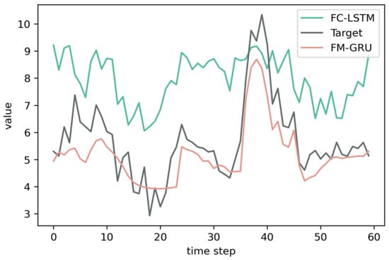
Figure 8.
Fitting comparison of the predicted value of dissolved oxygen.
4.6. Ablation Experiment
The core reason why the FM-GRU model proposed in this paper can still achieve better performance in the case of sparse data are that the FM model is more friendly to sparse matrices. The FM model can obtain high-dimensional interaction relationships between data, and the characteristics of the null data can also be obtained through other indicators, so the null value will not have a serious impact on the performance of the model. This section will study the influence of the FM model on the overall FM-GRU model. The research method is to test the performance of the model after removing the FM module on the same dataset to compare with the original FM-GRU model. We call the model after removing the FM module the Baseline Model, and the test results are shown in Table 3.
Table 3.
Performance comparison of the Baseline Model and FM-GRU.
Obviously, the model after removing the FM module has shown a significant decline in performance. This shows that the FM model does play an important role in the FM-GRU model proposed in this article, and it also provides a new problem-solving direction for the time series forecasting problem.
4.7. Impact of the Parameter K
The content to be discussed in this section is the influence of the hyperparameter K in the FM module on the performance of the model. K controls the width of the second-order interactive parameter matrix in the FM model, and we compare the error of the result by adjusting the value of K when the other parameters of the model are all the same. The test result (dissolved oxygen) is shown in Figure 9.
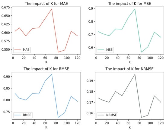
Figure 9.
Impact of parameter K on four error measurement indexes on the predicted value of dissolved oxygen.
The experimental results show that the performance of the model changes when the hyperparameter K takes different values. It can be seen that, when K = 84, the MSE is 0.56, and the model performs best at this time. According to the calculation principle of Factorization Machine, in general, the larger the value of the parameter K, the more adequate the fitting of high-dimensional features. However, since the value of K is the rank of the parameter matrix V, the larger the value of K, the more parameters of the V matrix will be, and the more training times will be required while the dataset used in this experiment only contains 1000 time steps, when the K value is set too high, the parameter matrix V cannot be learned enough, which makes the FM model unable to accurately fit the data. In addition because the value of K affects the size of the parameter matrix V, too large a value of K will increase the training time of the model and reduce the operating efficiency of the model, so the value of K should not be too large.
4.8. Impact of the Parameter Learning_Rate and Batch_Size
In this section, we explored the impact of learning rate and batch size on model performance. In deep learning, the traditional gradient descent calculates the loss of all samples every step, which will cause the generalization ability of the model to decrease, and, if the dataset is large, this solution will take up a lot of memory. However, the gradient descent method that only calculates the loss of one sample at a time is very unstable and often difficult to converge. Therefore, the idea of mini batch is widely used, this compromise solution avoids extreme situations and achieves good results in both efficiency and performance. The learning rate refers to the speed of parameter change when the model is training parameters. The size of the learning rate is very important for the predictive performance of the model. When the learning rate is too small, the loss function will be easier to obtain the minimum value, but the training process of the model will be very slow, affecting the efficiency of the model. While the learning rate is too large, the loss function often fluctuates around a larger value and cannot reach the minimum value, resulting in a decrease in the performance of the model. The question discussed in this section is what value of batch size and learning rate will achieve the best performance for the model. We take the batch_size in this experiment as seven commonly used values, which are 2, 4, 8, 16, 32, 64, and 128; the learning rate also takes three commonly used values, which are 0.001, 0.01, and 0.1, respectively. The experimental results are shown in Figure 10 (use RMSE as a measure).
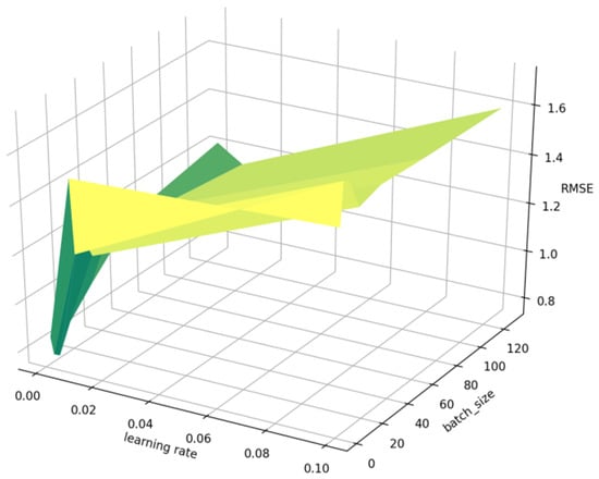
Figure 10.
Impact of the parameter batch_size and learning rate.
In Figure 10, we can see that, when batch_size = 8 and learning rate = 0.001, the model can achieve the best performance, which is in line with our expectations. If the batch size is too large or too small, it will have a negative impact on the performance of the model, while the learning rate is at 0.001, although the training time of the model will be longer, the model will reach the optimal effect and the error will reach the minimum.
4.9. Experiments on the Generalization Ability of the Model
Obviously, the ecological environment of each region is significantly different, and the water quality indicators are also very complicated, which leads to obvious differences in water quality data of different water bodies. Therefore, an excellent water quality prediction model should have strong generalization ability, so that it can handle different water quality data. The main content of this section is to verify whether FM-GRU has good generalization ability. The method we use is to change the dissolved oxygen, which was previously used as a prediction target, to a covariate, and use the PH value, which was previously used as a covariate, as our new prediction target. In this way, we get a brand new dataset (https://github.com/Adamkwang/FM-GRU) (accessed on 8 April 2021). Next, we use this new dataset to perform the same experiment on the above models as before, and record the experimental results. We record the results of this experiment in Table 4, in which we use bold fonts to highlight the best performance results. For brevity, we only use NRMSE as an indicator to measure performance.
Table 4.
Comparison of the performance of different methods in predicting the value of PH.
Apparently, the FM-GRU model we proposed in this paper still has better predictive performance than other models on a new dataset, and it has achieved a larger lead compared with other models. The excellent performance of FM-GRU on the new dataset proves that it has good generalization ability; this means that FM-GRU will also perform well in water quality datasets in different geographies.
5. Discussion of Experimental Results
Combining the results of the above multiple experiments, it can be seen that FM-GRU has indeed achieved good results in water quality prediction, and has achieved better prediction performance compared with previous statistics or machine learning methods. This proves that it is feasible to use the FM model to extract high-dimensional feature information of water quality data. By inputting this high-dimensional information into the seq2Seq model and applying double attention to it, FM-GRU can obtain more potential laws of the data itself and potential connections between the data than traditional deep learning models, so as to output results that are more accurate in the prediction stage. It is worth mentioning that XGBoost has shown excellent performance second only to FM-GRU in all the experiments of this paper, and it has opened a large gap with the remaining prediction methods. However, XGBoost often requires a long calculation time due to its implementation principle, which is very unfriendly to online forecasting, and it also places higher requirements on the hardware performance of the running equipment.
In future work, we plan to combine the ideas of XGboost and FM-GRU and optimize the overall implementation process to improve the operating efficiency of the model. At the same time, since CNN is an excellent feature extraction model, we will also try to use the concept of CNN to improve the high-dimensional potential information capture ability of our FM module, so as to further improve the predictive performance of the model.
6. Conclusions
In this paper, we propose a new model FM-GRU to deal with the problem of time series prediction of water quality data. FM-GRU technically realizes the effective integration of factorization machine and seq2seq framework, by using the FM model to solve the common problem of missing data in the water quality monitoring dataset and obtain the potential high-dimensional feature interactive information in the time series and process this information as input to the GRU model. At the same time, the dual-Attention added to the framework solves the long-range information loss problem of the traditional time series model, making the FM-GRU model still have a good effect on the time series analysis with a long-time span. In the experimental part, it can be seen that FM-GRU has obvious performance advantages in comparison with a variety of common time series forecasting schemes. At present, time series forecasting (TSF) and natural language processing (NLP) are one of the key research issues in academia and industry. This article proposes a new idea and method for solving TSF problems and NLP problems, and also for river water quality. Eco-environmental governance and planning have proposed new and effective solutions.
Author Contributions
K.W. and J.X. proposed the main idea and wrote the paper. K.W. and J.X. conceived the algorithm and designed a prediction framework. K.W. and C.L. performed the experiments and analyzed the results. L.X., X.H. and Y.Z. provided investigation and the dataset. All authors have read and agreed to the published version of the manuscript.
Funding
This research was funded by 2020 Li Ka Shing Foundation Cross-Disciplinary Research Grant (No. 2020LKSFG08D), the Shantou University Scientific Research Start-up Fund Project (No. NTF18024), and in part by a 2019 Guangdong province special fund for science and technology (“major special projects + task list”) project (No. 2019ST043).
Data Availability Statement
Data available in a publicly accessible repository that does not issue DOIs Publicly available datasets were analyzed in this study. This data can be found here: https://github.com/Adamkwang/FM-GRU.
Acknowledgments
We are grateful to three anonymous reviewers who have contributed to the enhancement of the paper’s completeness with their valuable suggestions.
Conflicts of Interest
The authors declare no conflict of interest.
References
- Son, G.; Kim, D.; Kim, Y.D.; Lyu, S.; Kim, S. A Forecasting Method for Harmful Algal Bloom (HAB)-Prone Regions Allowing Preemptive Countermeasures Based Only on Acoustic Doppler Current Profiler Measurements in a Large River. Water 2020, 12, 3488. [Google Scholar] [CrossRef]
- Terêncio, D.P.S.; Cortes, R.M.V.; Pacheco, F.A.L.; Moura, J.P.; Fernandes, L.F.S. A Method for Estimating the Risk of Dam Reservoir Silting in Fire-Prone Watersheds: A Study in Douro River, Portugal. Water 2020, 12, 2959. [Google Scholar] [CrossRef]
- Chang, D.L.; Yang, S.H.; Hsieh, S.L.; Wang, H.J.; Yeh, K.C. Artificial Intelligence Methodologies Applied to Prompt Pluvial Flood Estimation and Prediction. Water 2020, 12, 3552. [Google Scholar] [CrossRef]
- Hosmer, D.W., Jr.; Lemeshow, S.; Sturdivant, R.X. Applied Logistic Regression; John Wiley Sons: Hoboken, NJ, USA, 2013; Volume 398. [Google Scholar]
- Jaynes, E.T. On the rationale of maximum-entropy methods. Proc. IEEE 1982, 70, 939–952. [Google Scholar] [CrossRef]
- Cardoso, C.A.V.; Cruz, G.L. Forecasting natural gas consumption using ARIMA models and artificial neural networks. IEEE Lat. Am. Trans. 2016, 14, 2233–2238. [Google Scholar] [CrossRef]
- Tianliang, L.; Liming, H.; Haipeng, L. Prediction and analysis of chaotic time series on the basis of support vector. J. Syst. Eng. Electron. 2008, 19, 806–811. [Google Scholar] [CrossRef]
- Behzad, M.; Asghari, K.; Eazi, M.; Palhang, M. Generalization performance of support vector machines and neural networks in runoff modeling. Expert Syst. Appl. 2009, 36, 7624–7629. [Google Scholar] [CrossRef]
- Shiri, J.; Shamshirband, S.; Kisi, O.; Karimi, S.; Bateni, S.M.; Nezhad, S.H.H.; Hashemi, A. Prediction of water-level in the Urmia Lake using the extreme learning machine approach. Water Resour. Manag. 2016, 30, 5217–5229. [Google Scholar] [CrossRef]
- Yang, J.H.; Cheng, C.H.; Chan, C.P. A Time-Series Water Level Forecasting Model Based on Imputation and Variable Selection Method. Comput. Intell. Neurosci. 2017, 8734214. [Google Scholar] [CrossRef]
- Guo, T.; He, W.; Jiang, Z.; Chu, X.; Malekian, R.; Li, Z. An improved LSSVM model for intelligent prediction of the daily water level. Energies 2019, 12, 112. [Google Scholar] [CrossRef]
- Xiao, Q.; Si, Y. Time series prediction using graph model. In Proceedings of the 3rd IEEE International Conference on Computer and Communications (ICCC), Chengdu, China, 10–13 December 2017; pp. 1358–1361. [Google Scholar]
- Winata, G.I.; Kampman, O.P.; Fung, P. Attention-based lstm for psychological stress detection from spoken language using distant supervision. In Proceedings of the 2018 IEEE International Conference on Acoustics, Speech and Signal Processing (ICASSP), Calgary, AB, Canada, 15–20 April 2018; pp. 6204–6208. [Google Scholar]
- Ye, Q.; Yang, X.; Chen, C.; Wang, J. River Water Quality Parameters Prediction Method Based on LSTM-RNN Model. In Proceedings of the 2019 Chinese Control In addition, Decision Conference (CCDC), Nanchang, China, 3–5 June 2019; pp. 3024–3028. [Google Scholar]
- Dong, Q.; Lin, Y.; Bi, J.; Yuan, H. An Integrated Deep Neural Network Approach for Large-Scale Water Quality Time Series Prediction. In Proceedings of the 2019 IEEE International Conference on Systems, Man and Cybernetics (SMC), Bari, Italy, 6–9 October 2019; pp. 3537–3542. [Google Scholar]
- Tang, G.; Wu, Y.; Li, C.; Wong, P.K.; Xiao, Z.; An, X. A Novel Wind Speed Interval Prediction based on Error Prediction Method. IEEE Trans. Ind. Inform. 2020, 16, 6806–6815. [Google Scholar] [CrossRef]
- Barzegar, R.; Aalami, M.T.; Adamowski, J. Short-term water quality variable prediction using a hybrid CNN–LSTM deep learning model. Stoch. Environ. Res. Risk Assess. 2020, 34, 415–433. [Google Scholar] [CrossRef]
- Pan, M.; Zhou, H.; Cao, J.; Liu, Y.; Hao, J.; Li, S.; Chen, C.H. Water Level Prediction Model Based on GRU and CNN. IEEE Access 2020, 8, 60090–60100. [Google Scholar] [CrossRef]
- Baek, S.S.; Pyo, J.; Chun, J.A. Prediction of Water Level and Water Quality Using a CNN-LSTM Combined Deep Learning Approach. Water 2020, 12, 3399. [Google Scholar] [CrossRef]
- Wang, R.; Peng, C.; Gao, J.; Gao, Z.; Jiang, H. A dilated convolution network-based LSTM model for multi-step prediction of chaotic time series. Comput. Appl. Math. 2020, 39, 30. [Google Scholar] [CrossRef]
- Kutner, M.H.; Nachtsheim, C.J.; Neter, J. Applied linear regression model. Technometrics 2004, 26, 415–416. [Google Scholar]
- Turner, C.R.; Fuggetta, A.; Lavazza, L.; Wolf, A.L. A conceptual basis for feature engineering. J. Syst. Softw. 1999, 49, 3–35. [Google Scholar] [CrossRef]
- Rendle, S. Factorization machines. In Proceedings of the 2010 IEEE International Conference on Data Mining, Sydney, NSW, Australia, 13–17 December 2010; Volume 49, pp. 995–1000. [Google Scholar]
- Lyu, Z.; Dong, Y.; Huo, C.; Ren, W. Deep Match to Rank Model for Personalized Click-Through Rate Prediction. AAAI Conf. Artif. Intell. 2020, 34, 156–163. [Google Scholar] [CrossRef]
- Qin, J.; Zhang, W.; Wu, X.; Jin, J.; Fang, Y.; Yu, Y. User Behavior Retrieval for Click-Through Rate Prediction. arXiv 2020, arXiv:2005.14171. [Google Scholar]
- Xu, J.; Zheng, Z.; Lyu, M.R. Web service personalized quality of service prediction via reputation-based matrix factorization. IEEE Trans. Reliab. 2015, 65, 28–37. [Google Scholar] [CrossRef]
- Vaswani, A.; Shazeer, N.; Parmar, N.; Uszkoreit, J.; Jones, L.; Gomez, A.N.; Polosukhin, I. Attention is all you need. Adv. Neural Inf. Process. Syst. 2017, 30, 5998–6008. [Google Scholar]
- Cho, K.; Van Merriënboer, B.; Gulcehre, C.; Bahdanau, D.; Bougares, F.; Schwenk, H.; Bengio, Y. Learning phrase representations using RNN encoder-decoder for statistical machine translation. arXiv 2014, arXiv:1406.1078. [Google Scholar]
- Chung, J.; Gulcehre, C.; Cho, K.; Bengio, Y. Empirical evaluation of gated recurrent neural networks on sequence modeling. arXiv 2014, arXiv:1412.3555. [Google Scholar]
- Montgomery, D.C.; Peck, E.A.; Vining, G.G. Introduction to Linear Regression Analysis; John Wiley Sons: Hoboken, NJ, USA, 2012; Volume 821. [Google Scholar]
- Chen, T.; Guestrin, C. Xgboost: A scalable tree boosting system. In Proceedings of the 22nd ACM Sigkdd International Conference on Knowledge Discovery and Data Mining, San Francisco, CA, USA, 13–17 August 2016; pp. 785–794. [Google Scholar]
- Sutskever, I.; Vinyals, O.; Le, Q.V. Sequence to sequence learning with neural networks. Adv. Neural Inf. Process. Syst. 2014, 27, 3104–3112. [Google Scholar]
Publisher’s Note: MDPI stays neutral with regard to jurisdictional claims in published maps and institutional affiliations. |
© 2021 by the authors. Licensee MDPI, Basel, Switzerland. This article is an open access article distributed under the terms and conditions of the Creative Commons Attribution (CC BY) license (https://creativecommons.org/licenses/by/4.0/).