Article

Spatial and Temporal Shifts in Historic and Future Temperature and Precipitation Patterns Related to Snow Accumulation and Melt Regimes in Alberta, Canada

1
Airshed and Watershed Stewardship Branch, Resource Stewardship Division, Alberta Environment and Parks, 3535 Research Road NW, Calgary, AB T2L 2K8, Canada
2
Environmental Knowledge and Prediction Branch, Resource Stewardship Division, Alberta Environment and Parks, 3535 Research Road NW, Calgary, AB T2L 2K8, Canada
*
Author to whom correspondence should be addressed.
Water 2021, 13(8), 1013; https://doi.org/10.3390/w13081013
Submission received: 26 February 2021 / Revised: 30 March 2021 / Accepted: 1 April 2021 / Published: 7 April 2021
(This article belongs to the Special Issue Past and Future Trends and Variability in Hydro-Climatic Processes)

Abstract

:
Shifts in winter temperature and precipitation patterns can profoundly affect snow accumulation and melt regimes. These shifts have varying impacts on local to large-scale hydro-ecological systems and freshwater distribution, especially in cold regions with high hydroclimatic heterogeneity. We evaluate winter climate changes in the six ecozones (Mountains, Foothills, Prairie, Parkland, Boreal, and Taiga) in Alberta, Canada, and identify regions of elevated susceptibility to change. Evaluation of historic trends and future changes in winter climate use high-resolution (~10 km) gridded data for 1950–2017 and projections for the 2050s (2041–2070) and 2080s (2071–2100) under medium (RCP 4.5) and high (RCP 8.5) emissions scenarios. Results indicate continued declines in winter duration and earlier onset of spring above-freezing temperatures from historic through future periods, with greater changes in Prairie and Mountain ecozones, and extremely short or nonexistent winter durations in future climatologies. Decreases in November–April precipitation and a shift from snow to rain dominate the historic period. Future scenarios suggest winter precipitation increases are expected to predominantly fall as rain. Additionally, shifts in precipitation distributions are likely to lead to historically-rare, high-precipitation extreme events becoming more common. This study increases our understanding of historic trends and projected future change effects on winter snowpack-related climate and can be used inform adaptive water resource management strategies.

1. Introduction

Winter climate dynamics including sustained below-freezing temperatures and snow accumulation are critical for the seasonal redistribution of freshwater in many hydrological systems in western Canada, especially those with mountainous, high elevation headwaters. The accumulation of snow in alpine headwaters acts as a large and transient natural reservoir, gradually supplying fresh water to downstream regions during the warm season as a function of elevation and aspect controls on both snow accumulation and melt [1]. Multiple studies demonstrate that climate has changed over recent decades and is projected to continue to change, particularly during winter months [2,3]. These shifts will have profound impacts on the spatial and temporal distribution of freshwater sourced from snow melt [4,5]. As a result, concern has been raised over the potential for widespread downstream impacts on water resource availability due to changes in snowpack regimes over mountain environments and the implications for adaptive water resource monitoring and management [6,7].
Potential shifts in water resources in western Canada will have impacts on key economic drivers including agriculture, hydroelectric power and forestry as well as implications for municipal water supplies, recreation, and extreme event resilience. Additionally, changes to cold season temperature and precipitation can have considerable impacts on hydro-ecological systems downstream of mountain headwater regions. On a local or regional scale, shifting snow accumulation and melt regimes will affect aquatic and terrestrial ecosystems [8], groundwater recharge [9,10], wetland water balance [11,12], and glacier mass balance [13]. However, our understanding of how shifting winter temperature and precipitation patterns may affect snow accumulation and melt in different regions is limited.
Among the concerns with rising winter temperatures is an increase in the likelihood of fluctuations above and below freezing, and associated risk of snowpack loss [14,15,16]. Probabilities of snow accumulation and melt are strongly influenced by air temperatures near 0 °C [17], and the possibility of rain on snow rises with above-freezing temperatures [18], which can lead to extreme hydrologic events [19,20]. Warmer mean winter temperatures also affect the temperature of the snowpack; a warmer snowpack will melt faster than a cold snowpack as initial energy inputs to a cold snowpack are first used to raise the temperature of the snowpack to 0 °C isothermal before energy can be used for a phase change to liquid water [21]. While the development of winter snowpack is driven by temperature and precipitation, spring snowmelt dynamics are largely a function of energy inputs, solar radiation being the dominant driver [22]. Although several studies have detected an earlier spring freshet [23,24], there is not a simple linear relationship between rising temperatures, snowmelt, and hydrologic responses. Due to solar energy limitations during winter and early spring, rising temperatures and an earlier onset of above-freezing temperatures result in a slower rate of snowmelt [22,25], effectively weakening relationships between snowpack regimes and spring hydrology [26,27].
The IPCC Fifth Assessment Report projects a global annual temperature increase of 1.8 °C for RCP 4.5 and 3.7 °C for RCP 8.5 by 2100, relative to a 1986–2005 baseline climatology [28]. These projections do not account for considerable geographic and seasonal variability, and the greatest rates of warming are projected for winter months and high latitude regions. Canada’s Changing Climate Report scales down climate projections to geographic regions in Canada, including an increase in annual temperature of 1.9 and 6.5 °C averaged over the Prairie Provinces (Alberta, Saskatchewan, and Manitoba) by 2100 for RCP 2.6 and RCP 8.5, respectively [3]. Historic trend analyses on winter temperatures have documented a temperature increase in western Canada since the mid-20th century [29,30,31] and future climate projections consistently forecast continued increases, the magnitude of which depends on the future time period and emissions scenario [3,5,32]. Concomitant with increasing temperatures have been decreases in winter precipitation [29,30], snowfall [33,34], and snow water equivalent (SWE) [35] over the historic period. Conversely, winter precipitation is projected to increase [3,5], while snow cover fraction and SWE are projected to decrease [2,36]. Although historic and future climate change rates are commonly averaged over a regional [3] or watershed scale [5,32], it is clear that there is considerable spatial variability in the magnitude of temperature and precipitation changes. There is a need to scale analyses to Alberta to better understand how climate and water resource distribution has and is projected to change.
Here we focus on the Province ofIn Alberta as the eastern slopes of the Rocky Mountains serve as the headwaters of several major rivers in Canada that flow to the Arctic Ocean (the Peace and Athabasca Rivers) and Hudson Bay (the North and South Saskatchewan Rivers). As a result, regional hydroclimatic changes in Alberta have water availability implications across western and northern Canada and the potential to affect the Arctic Ocean freshwater balance [37,38]. Freshwater has critical ecological and socioeconomic importance in the Province, providing essential resources for municipal, industrial, agricultural, and recreational and traditional uses as well as aquatic and terrestrial ecosystem habitats. Even minor changes in the seasonal or geographic distribution of fresh water can have cumulative impacts on hydrological and ecological systems [39]. Given the heterogeneity of regional contributions to streamflow in major Albertan river basins and the unequal rates of temperature and precipitation changes, this study focuses on quantifying historic and projected changes in winter climate by ecological zones in Alberta. Quantification of these changes is based on key temperature and precipitation metrics to characterize winter climate using high resolution gridded climate data, including winter duration, the timing of spring above-freezing temperatures, total precipitation and snowfall. A Mann–Kendall (MK) trend analysis is applied to evaluate winter climate trends over the historic period and departures from the historic baseline are calculated for future scenarios. Results of this research will inform potential hydrologic impacts of climate change in different biogeographic regions within major watersheds. Moreover, results will identify regions that are projected to become disproportionately affected by changing climate.

2. Materials and Methods
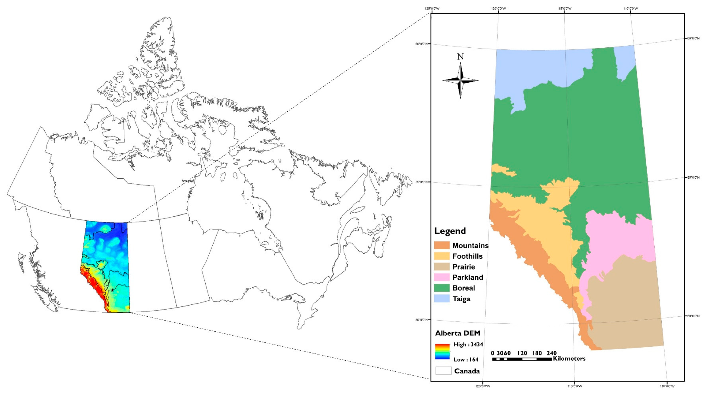
2.1. Study Area

The physiographic and biogeoclimatic diversity in Alberta is represented by six ecological regions defined by the Ecological Framework of Canada (Figure 1) [40]. Mountain, Prairie, Boreal, and Taiga are all ecozones under the framework, where Parkland is an ecoregion within the Prairie ecozone and Foothills is an ecoregion within the Boreal ecozone. Hydroclimatic changes in these ecoregions can have distinct regional impacts; therefore, they are distinguished as separate zones for the purposes of this research. These six zones will all be referred to as ecozones throughout the manuscript.
There are pronounced climatic gradients among Alberta’s ecozones, with the highest mean cold season (November–April) precipitation occurring in the Mountains (214 mm) and lowest in the Prairie (87 mm) ecozone, and highest mean November–April temperature in the Prairie (4.2 °C) and lowest in the Taiga (−2.2 °C) ecozone (Table 1). Mean climate within ecozones is also variable, particularly in the Mountain ecozone for both temperature and precipitation, while the greatest homogeneity for precipitation is in the Taiga ecozone and for temperature in the Parkland ecozone. The Mountain ecozone, characterized by steep, rocky terrain and alpine-subalpine ecosystems, has the highest mean elevation (1890 m) and greatest elevation range (860–3630 m). This is also the smallest ecozone in the province, approximately 47,000 km2. The adjacent ecozone, Foothills, is a transitional region between mountains and low-elevation forest and grassland. Elevations range from 600–2450 m, typified by rolling hills and broad valleys. Numerous parks and protected areas exist in the Foothills and Mountain ecozones. Additionally, many large dams and reservoirs are located in the Foothills, making this zone a critical region for water management.
The plains ecozones—Prairie, Parkland, Boreal, and Taiga, have relatively low elevation profiles and south-north climate gradients (Table 1). The Prairie ecozone largely consists of natural mixed grassland and numerous wetlands in topographic depressions, which rely on the accumulation of snow and snowmelt runoff [41]. The Parkland ecozone represents a transition zone between Prairie grassland and Boreal forest. Both the Prairie and Parkland ecozones have productive agriculture sectors, which are highly dependent on water, and water management practices, including diversions, withdrawals, and irrigation. Northern Alberta is largely covered by the Boreal and Taiga ecozones. The Boreal ecozone is dominated by a hummocky landscape with numerous lakes and extensive forest. Both the Boreal and Taiga ecozones contain significant wetlands areas and sporadic discontinuous permafrost and are characterized by poor drainage.

2.2. Data

2.2.1. Historic Period

To generate key historic winter air temperature and precipitation metrics, high-resolution (approximately 10 km) gridded daily minimum and maximum air temperature and daily precipitation data for Canada, developed using the ANUSPLIN multidimensional interpolation method [42,43], are used. This method uses a trivariate thin-plate spline algorithm that accounts for topographic variability by using elevation as the third predictor variable [42,43]. The accuracy of the gridding procedure was assessed using data from climate stations withheld from the initial gridding stage, and these withheld stations were incorporated into the final gridding procedure [42,43]. The original ANUSPLIN dataset covered the time period from 1961–2003 [42] and improvements were made to the dataset which reduced the residuals between observations and interpolated values and extended the dataset to 1950–2007 [44]. The present dataset is available for 1950–2017. These data have been widely used for climate change analyses, e.g., [30,45,46,47] and hydrologic modelling, e.g., [48,49]. Additionally, ANUSPLIN datasets have been used to statistically downscale global climate models (GCMs) for Canada, e.g., [50,51].
In Canada, a higher density of climate stations exists at lower elevations and latitudes, with stations often established in relatively accessible locations. Consequently, the distance between stations at high latitudes and elevations is greater, leading to lower confidence in interpolating data in these regions, particularly high elevations due to complex topography [52]. A dry and cold bias in the historic ANUSPLIN data was identified over mountainous regions of western Canada [48,53,54], with the dry precipitation bias stronger during the winter season [55]. However, further studies in western Canada comparing ANUSPLIN gridded climate data with similar observation-based interpolated data and reanalysis data have concluded that ANUSPLIN performs well and is the best available data [53,54,55]. Therefore, a spatial subset of the ANUSPLIN dataset covering Alberta for 1950–2017 is used for analysis of historic climate.

2.2.2. Future Period

Two future periods are evaluated, the 2050s (2041–2070) and the 2080s (2071–2100), for two representative concentration pathways (RCPs), RCP 4.5 and RCP 8.5. Each future period represents a 30-year climatology from which the mean and distribution of climate variables can be calculated and compared with the historic baseline period (1950–2017). RCP 4.5 is a ‘medium-low’ stabilization scenario that accounts for a rise in radiative forcing over coming years followed by a plateau through 2100, while RCP 8.5 maintains status quo and represents a rise in radiative forcing through 2100 [56].
In this study, multiple GCMs with different radiative forcing scenarios are selected based on an envelope approach which relies on capturing a wide range of simulated changes for a number of climatological variables of interest [57,58,59]. The aim of this approach is to select an ensemble of GCM scenarios that covers all possible future conditions projected by the entire pool of climate models [60]. The envelope approach used in this study is an integrated computational geometry algorithm (QH-RDP) [59]. The QH-RDP algorithm is used to identify the smallest ensemble that preserves the maximum spread of the projection of an initial pool (the largest available) of phase 5 of the Coupled Model Intercomparison Project (CMIP5) run with RCP 4.5 and RCP 8.5 scenarios (Table 2).
The QH-RDP algorithm (described in detail in [59]) was developed to determine a subset of GCM simulations that cover the spread of projection, based on integrating the QuickHull and Ramer–Douglas–Peucker algorithms:
(1) The QuickHull algorithm is a geometry method of computing the convex hull of a finite set of points in n-dimensional space. This algorithm is used to identify GCM scenarios that uniformly cover the multivariate distribution of GCM scenarios for the selected climatic indices, with an emphasis on selection of those that lie on the edges of the distribution in a high-dimensional space.
(2) The Ramer–Douglas–Peucker (RDP) algorithm is a computer cartography algorithm for shape simplification which is used to capture the most prominent extreme GCMs. In other words, the convex set (the initial ensemble) selected by the QuickHull algorithm can still be shrunk, if possible, to even smaller ensembles by the RDP algorithm.
A total of six GCM scenarios are selected whereas the conservation of the projection spread is confirmed using a robust validation method [59,61] when the spread error is calculated for each simulation run. The ensemble of GCM scenarios, which preserve the maximum spread of the projection, consists of MIROC-ESM-CHEM, MPI-ESM-MR, and FGOALS-g2 for the RCP 4.5 scenario and MIROC-ESM, CSIRO-Mk3-6-0, and CanESM2 for the RCP 8.5 scenario. Projections of minimum and maximum daily surface air temperature and precipitation, statistically downscaled using the ANUSPLIN gridded historic period dataset [51], were downloaded for Alberta from the Pacific Climate Impacts Consortium website [62].

2.3. Methods

2.3.1. Temperature Metrics

Temperature metrics that characterize winter climate related to snow accumulation and melt are calculated for historic and future periods. Daily minimum and maximum surface air temperatures are averaged to estimate mean daily temperature. Mean daily air temperatures are used to calculate the onset of below and above freezing temperatures to determine the timing of the spring 0 °C isotherm and winter duration. Winter duration largely dictates the length of the snow accumulation season, although there are processes throughout winter, including mid-winter thaw episodes and snow redistribution that affect snowpack development [63,64]. The spring 0 °C isotherm signifies the onset of snowmelt and spring freshet. Autumn and spring temperatures typically fluctuate above and below freezing, which can result in short-term variations between snow-rain and freeze-melt during this transition. Following the methods outlined in [65], a 31-day running mean of daily temperatures is calculated to smooth fluctuations above and below freezing during autumn and spring. The 0 °C isotherm dates are defined as the day when the 31-day running mean rises above the 0 °C threshold in spring and below this threshold in the autumn. Where multiple threshold crossings still exist, the 0 °C isotherm date is defined as the last 0 °C crossing in spring, and first 0 °C crossing in autumn [65]. Winter duration is calculated as the number of days between the autumn and spring 0 °C isotherm dates.
For the historic period (1950–2017), spring 0 °C isotherm dates and winter duration are evaluated using the MK nonparametric test for trend [66,67]. The trend magnitude is determined using Sen’s slope estimator, which is insensitive to outliers [68]. Statistical significance is evaluated at the 5% level. The MK test has been widely used in hydroclimatic trend analyses, e.g., [30,69]. Long-term records are preferable for trend analyses as climate is nonstationary and influenced by low-frequency modes of variability [24,70]. In cases where hydrologic or climate data are autocorrelated, the MK test may falsely detect a trend [71]. It has been common to apply a prewhitening procedure to remove autocorrelation for analyses of environmental data. Historic climate data are evaluated for autocorrelation and guidelines outlined in [71], including sample size, trend slope, and coefficient of variation. It was concluded that prewhitening should not be performed for this analysis.
For each future period, ensemble mean values for the spring 0 °C isotherm and winter duration are evaluated, and the departure from the historic baseline period calculated. Temperature and precipitation can exhibit persistent multi-year to decadal variability, which influence calculations of mean conditions over short periods; therefore, the full historic period (1950–2017) is used for the historic baseline period. While the mean value provides information about average conditions, metrics of variability indicate the range of projected conditions, including standard deviation from the mean and the high and low ends of the distributions of each climate variable. Changes to variability indicate whether the tail ends of the distributions are shifting closer to or further from the mean value, demonstrating projected risks of very early or late spring onset or very short or long winter duration. The 10th and 90th percentiles represent the lower and upper tails of the distribution, respectively. In a 30-year climatology, the 10th percentile represents the threshold below which the values for the three shortest winters and earliest spring onsets occur in the distribution. Similarly, the 90th percentile represents the threshold separating the three longest winters and latest spring onsets. Standard deviation represents a range above and below the mean value in which the majority of values occur, and together with the 10th and 90th percentiles are indicative of the overall shape of the distribution. These metrics of variability are calculated for spring 0 °C isotherm and winter duration for each future period and scenario, relative to the historic baseline conditions. Changes in variability are evident by comparing the magnitude of change in standard deviation and 10th and 90th percentiles between historic and future scenarios.

2.3.2. Precipitation Metrics

Two metrics are used to represent cold season (November–April) precipitation; total precipitation and snowfall. While changes in total winter precipitation are important, changes in precipitation phase, or the covariability of temperature and precipitation, are indicative of the development of winter snowpack. Snowfall is calculated using a temperature-index precipitation phase algorithm with a threshold temperature of 1 °C. Precipitation falling on days when the mean daily temperature is below 1 °C is counted as snow, and otherwise is considered rain. Rain may occur below and snow above 1 °C, influenced by humidity [21,72,73] and overlying air mass movement [74]. Although precipitation phase uncertainty is largest for temperatures between 0 and 2 °C [74], and there is seasonal [75] and spatial [76] variability, a 1 °C threshold maximizes accuracy over a large spatial domain [77] and is consistent with studies in similar regions [17,77,78,79,80]. Cumulative snowfall is calculated as the sum of all November–April precipitation that falls on days when the temperature is below the given threshold. Historic total precipitation and snowfall trends are calculated using the MK test, evaluated at the 5% significance level [66,67,68].
Projected changes in cold season (November–April) precipitation are evaluated relative to the range of mean daily temperatures. Daily mean temperatures are rounded to the nearest degree and the range of temperatures is used as “bins.” The sum of all precipitation values for each “bin” is calculated. For example, if the temperature is −20 °C during 10 days between November and April, the precipitation for those 10 days is summed to give the total amount of precipitation for that temperature “bin”. The temperature “bins” are ranked from low to high and cumulative precipitation is calculated and averaged for an ensemble mean for each future period and scenario. Representing projected changes in precipitation in this manner facilitates the evaluation of projected changes in total precipitation and the proportion of precipitation that falls as snow. The advantage of this method is the ability to determine how much precipitation falls below certain temperatures, such as the 1 °C rain–snow threshold, and the range and distribution of temperatures at which precipitation occurs. This is critical not only for precipitation phase evaluation, but also to make inferences about the temperature of the snowpack. It is important to note that temperature and precipitation distributions are not given as a time series. Temperatures may fluctuate above and below freezing throughout the cold season, particularly in during the transitions between autumn–winter and winter–spring. Therefore, cumulative precipitation below 1 °C should not be interpreted as winter snow accumulation or SWE.

3. Results

3.1. Historic Climate

Widespread significant (p < 0.05) negative trends are detected across Alberta for the spring 0 °C isotherm and winter duration over the historic period, signifying an earlier onset of above-freezing temperatures and shorter winter duration (Figure 2). The magnitude of trends vary within ecozones and across the province, with strong north-south gradients. Winter duration represents an integration of changes to autumn and spring 0 °C isotherm dates. Although no statistically significant trends are found for autumn 0 °C isotherm dates (not shown), the higher trend magnitudes for winter duration compared with spring 0 °C isotherm suggest a later onset of below-freezing temperatures. The greatest trends are seen in the Prairie ecozone in southern Alberta, where spring 0 °C isotherm has become earlier at rates up to 3.4 days per decade and winter duration has decreased by up to 4.3 days per decade. Over the duration of the historic period, this corresponds to a shift of approximately 3 weeks earlier for the onset of above-freezing temperatures and 4 weeks shorter duration of below-freezing temperatures. Conversely, the smallest trends are seen in the Taiga ecozone where decreasing trends as low as 1 day per decade are detected for both spring 0 °C isotherm and winter duration. Trends toward earlier spring 0 °C isotherm and shorter winter duration are highly variable in the Foothills ecozone, with larger trend magnitudes along the western edge. In contrast, the neighboring Mountain ecozone is characterized by low trend magnitudes for the spring 0 °C isotherm and a noticeable absence of trends for winter duration, with the exception of the southern Mountains. Large portions of the Parkland and Boreal ecozones exhibit no statistically significant trends for winter duration and low to moderate negative trends for spring 0 °C isotherm timing.
Two cold season (November–April) precipitation metrics are evaluated to understand how total precipitation (Pt) and snowfall (Ps) have changed over the historic period. The concomitant trends in total precipitation and snowfall are indicative of shifts in precipitation phase in addition to changes in total precipitation. Trend magnitudes for total November–April precipitation are given on the x-axis and snowfall on the y-axis (Figure 3). Statistical significance (p < 0.05) is shown for trends in snowfall (y-axis), and most of these points are also statistically significant for trends in total cold season precipitation. The reference lines indicate equal trend magnitude (Pt = Ps); points that fall below the reference line signify where Pt < Ps. In other words, for negative trend values, points below the reference line indicate that decreases in snowfall exceed that of total precipitation and thus a shift from snow to rain accompanies a loss of total precipitation. Points above the reference line indicate that loss of total cold season precipitation has largely come at the expense of rain rather than snow.
An overall decrease in both total precipitation and precipitation falling when the mean daily temperature is below 1 °C is detected for all ecozones (Figure 3). Few increasing trends in total precipitation are detected, and these occur in all ecozones except the Foothills. Additionally, increases in snowfall for parts of the Mountain ecozone occurred, although these increasing trends are not statistically significant at the 5% level. Trend magnitudes closely track the Pt = Ps reference line for the Taiga ecozone, indicating total precipitation losses are nearly entirely seen as a loss of snowfall. Similarly, trend magnitudes in the Mountain ecozone follow a linear pattern just below the reference line indicating a slight shift from snow to rain nested within the overall precipitation decreases and increases. Significant decreasing trends in the Foothills ecozone are spread above and below the reference line meaning that while some grid points have shifted from snow to rain, others have shifted from rain to snow. However, the ecozone average indicates an overall loss of snow and a loss of total precipitation. The greatest departure from the reference line for ecozone averaged trend magnitudes are found in the Parkland and Prairie ecozones, indicating a larger shift from snow to rain superimposed over decreasing precipitation trends.

3.2. Future Climate

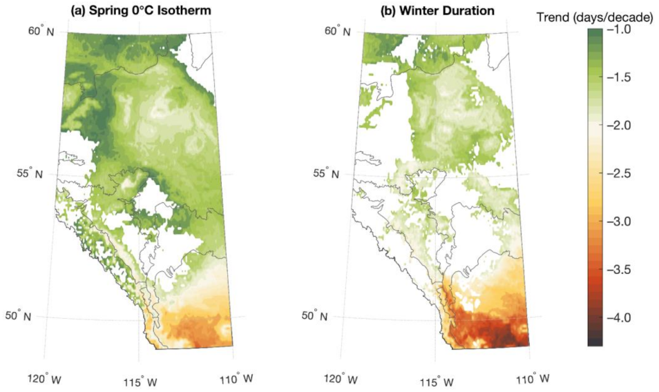
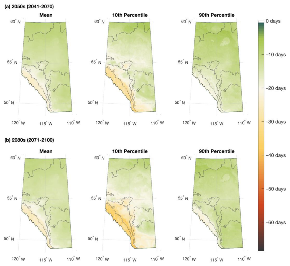
3.2.1. Spring 0 °C Isotherm

Future climate projections, based on the RCP 4.5 and RCP 8.5 scenarios reveal substantial increases in temperature-related indices affecting winter climate in Alberta. Mean, 10th and 90th percentiles of spring 0 °C isotherm dates are projected to shift earlier in the 2050s and 2080s for both RCP 4.5 (Figure 4) and RCP 8.5 (Figure 5). The largest changes are projected for the southwestern region of Alberta, in the Mountain ecozone and to a slightly lesser extent the Foothills ecozone. Ecozone-averaged decreases in mean spring 0 °C isotherm dates for all ecozones are similar for both the RCP 4.5 and RCP 8.5 scenarios for the 2050s and the RCP 4.5 scenario for the 2080s (Table 3). However, the magnitude of change diverges substantially for the 2080s under the RCP 8.5 scenario. For example, the mean spring 0 °C isotherm date in the Foothills ecozone is projected to become 18–19 days earlier in the 2050s for both RCP 4.5 and RCP 8.5 and in the 2080s for RCP 4.5, initiating spring melt in mid-March while the 2080s RCP 8.5 scenario projects a decrease of 31 days, to early March. The smallest change occurs in the Taiga ecozone, which is projected to be 10 days earlier in the 2050s for both scenarios and 11 or 16 days earlier in the 2080s for RCP 4.5 and RCP 8.5, respectively. Conversely, the largest shift, in the Mountain ecozone, projects 23 or 26 days earlier for RCP 4.5 and RCP 8.5 in the 2050s, and 25 or 39 days earlier in the 2080s.
Changes in variability of spring 0 °C isotherm dates are evaluated as the magnitude of change in standard deviation and 10th and 90th percentiles relative to the historic period, summarized in Table 3. Metrics of variability indicate the extreme high and low values that exist in the future climatologies and provide a more comprehensive picture of what is in the expected realm of climate change than only evaluating mean values. The spread of the distributions of annual spring 0 °C isotherm dates for all ecozones are projected to narrow closer to the mean for the majority of values, evident by a decreases in standard deviation, except for the 2080s under RCP 8.5 where standard deviations are projected to increase for Mountain, Foothills, and Boreal ecozones. Distributions are also projected to skew toward the lower end, demonstrated by a higher magnitude of change between the historic and future periods for the 10th percentile (earliest spring onset) compared to changes in the mean. Conversely, the magnitude of changes for the 90th percentile (latest spring onset) is lower than the change in mean between historic and future periods for all ecozones. For example, in the 2050s for the Parkland ecozone, the mean spring 0 °C isotherm date is projected to become 14 or 16 days earlier for RCP 4.5 and RCP 8.5, respectively. Additionally, the 10th percentile date is projected to shift 16 or 23 days earlier while the 90th percentile is only projected to become 14 or 12 days earlier, and the standard deviation decreases by 3.5 or 3.2 days. The 10th percentile, representing an early spring 0 °C isotherm, are projected to become much earlier in all future scenarios, particularly for RCP 8.5 in the 2080s period, ranging from 19 days in the Taiga ecozone to 54 days in the Mountain ecozone. This means that in the 2080s in the Mountain ecozone, ten percent of spring 0 °C isotherm dates will occur by mid-February, which could have profound impacts on snow accumulation and melt regimes.

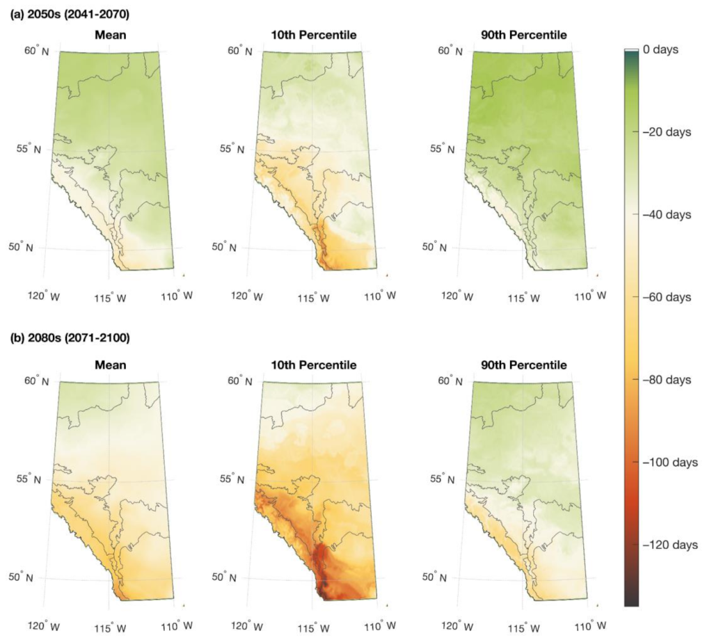
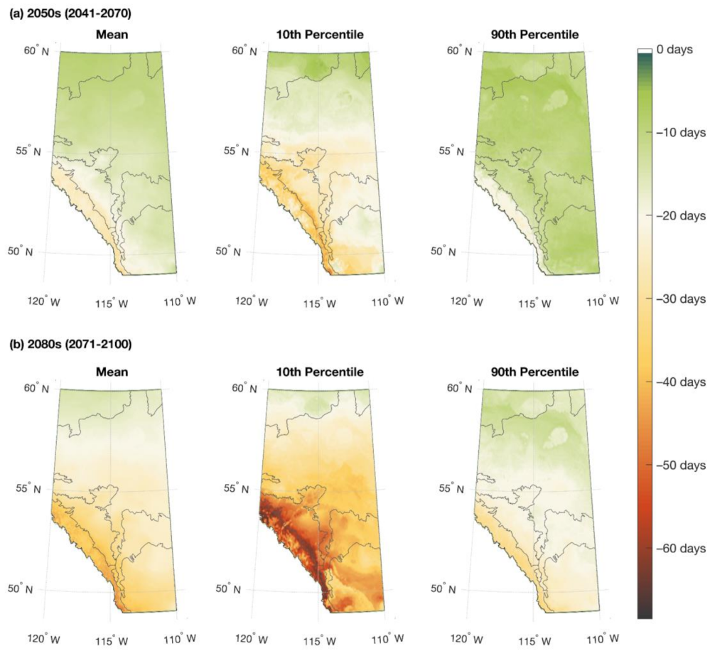
3.2.2. Winter Duration

Projected decreases in winter duration are largely driven by spring 0 °C isotherm dates combined with moderate changes in autumn 0 °C isotherm dates (Supplementary Information). Spatially, the largest changes are projected to occur in the southwestern region of the province for both the 2050s and 2080s for RCP 4.5 (Figure 6) and RCP 8.5 (Figure 7). Patterns of high-magnitude changes are ubiquitous in the Mountain and Foothills ecozones, relative to other parts of the province, with decreases in mean winter duration of up to 41 and 60 days in the 2050s and 44 and 90 days in the 2080s for RCP 4.5 and RCP 8.5, respectively. There is a small range of ecozone-averaged projected decreases in winter duration between the RCP 4.5 and RCP 8.5 scenarios for the 2050s and the RCP 4.5 scenario for the 2080s (Table 4). For example, in the Taiga ecozone losses of 17 to 20 days are expected, where the Mountain ecozone is projected to decrease by 33 to 44 days. However, projections for the 2080s under RCP 8.5 diverge considerably from this range. Decreases of 69 days are projected for the Mountain ecozone, and losses of more than 50 days are projected for the Prairie, Foothills, and Parkland ecozones. For ecozones with typically shorter winter duration, such as the Prairie zone, the predicted reduction in winter duration by 60 days results in a mean winter duration decline of ca. 44% from the historical average of 136 days. Similarly, the Mountain ecozone is projected to experience a 37% decline in winter duration from 187 days over the historical period to a mean duration of just 118 days by the 2080s.
Projected changes in variability, demonstrating the expected range of future conditions, in winter duration are of particular concern, especially for the low ends of the distribution, or extremely short duration, given by the 10th percentile (Table 4). While the magnitude of projected changes in the 90th percentile are close to mean values, the magnitude of changes in the 10th percentile considerably exceed that of the mean, indicating the projected shifts are skewed toward the low extremes. For example, the 10th percentile for the Boreal ecozone is projected to be 26 or 37 days earlier in the 2050s for RCP 4.5 and RCP 8.5, respectively, while the 90th percentile is projected to shift 17 days earlier for both RCP scenarios. The largest change in variability is seen in the 2080s for RCP 8.5 where the 10th percentile in winter duration is projected to decrease with a range of 39 days in the Taiga ecozone to 88 days in the Mountain ecozone. For the Mountain ecozone this results in a winter duration of less than 80 days for 10 percent of winters in the 2071–2100 period. Similar large projected decreases for this period lead to 10 percent of winters lasting less than 32, 58, and 62 days for Prairie, Foothills, and Parkland ecozones. Standard deviations, indicating how close to the mean the majority of values occur, are projected to decrease in the 2050s for RCP 4.5 for all ecozones and RCP 8.5 for the Prairie, Parkland, and Taiga ecozones, signifying a decrease in variability. Similarly, for the 2080s, standard deviations are projected to decrease for all ecozones under RCP 4.5, but increases in standard deviation, and therefore variability, are projected for all ecozones except the Prairie for RCP 8.5.
The disproportionate rate of change in the Mountain ecozone will alter spatial gradients in spring 0 °C isotherm timing and winter duration across the province. During the historic period, the average onset of above-freezing temperatures in the Mountain ecozone (22 April) occurred just a few days after that of the Taiga ecozone (18 April) and up to 30 days following that of the Prairie ecozone (23 March) (Table 3). This is projected to shift such that the timing of the spring 0 °C isotherm in the Mountain ecozone will be 9 to 19 days later than the Taiga ecozone between RCP 4.5 in the 2050s to RCP 8.5 in the 2080s, and 20 or 21 days after the Prairie ecozone. Similar patterns exist for winter duration, where the historic period is characterized by a roughly equivalent average winter duration for Mountain (187 days) and Taiga (183 days) ecozones to a large difference between Mountain (187 days) and Prairie (136 days) ecozones (Table 4). Under future projections, the difference in mean winter duration for Mountain and Taiga ecozones will diverge and converge for Mountain and Prairie ecozones. Ranging from the 2050s for RCP 4.5 and 2080s for RCP 8.5, mean winter duration in the Mountain ecozone will become 12 to 33 days shorter than the Taiga ecozone, while the gap between the duration of Mountain and Prairie ecozones will shorten by 7 to 9 days. Future scenarios suggest that the winter duration and spring 0 °C isotherm in the Mountain ecozone will become more similar to that of the Boreal ecozone.
The Prairie ecozone also emerges as a region projected to experience a high rate of change in winter duration relative to other ecozones, a pattern that is not seen with spring 0 °C isotherm projections, suggesting a larger shift in the timing of the autumn 0 °C isotherm, or onset of below-freezing temperatures (Supplementary Information). These projected changes are pronounced for the 10th percentile, particularly under RCP 8.5, where decreases of over 120 days are projected for southwestern Alberta. Given the substantial projected decreases in the low end of the distribution of winter duration, as demonstrated by the 10th percentile results, particularly for RCP 8.5 and the 2080s, we evaluated the projected percentage of years that remain above freezing throughout the winter. In these cases, no autumn or spring 0 °C isotherms are detected. Results indicate that small areas of the Prairie ecozone are not projected to freeze for a small percentage (<10%) of years between 2041–2070 for RCP 8.5 and 2071–2100 for RCP 4.5 (Figure 8). A widespread region of southern Alberta, extending across multiple ecozones (<10%) and a high concentration in the southwestern Prairie ecozone (up to 21%) is projected to remain above freezing between 2071–2100 for RCP 8.5. As 0 °C isotherm dates are calculated using a 31-day running mean there may still be short-term fluctuations above and below freezing, such as daily or multi-day time scales. However, no sustained cold periods are projected to occur under these scenarios.

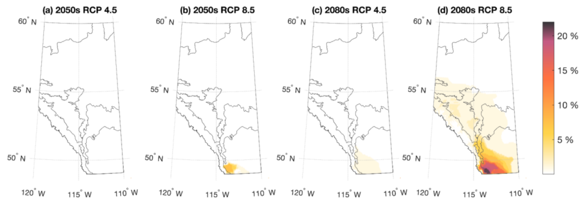
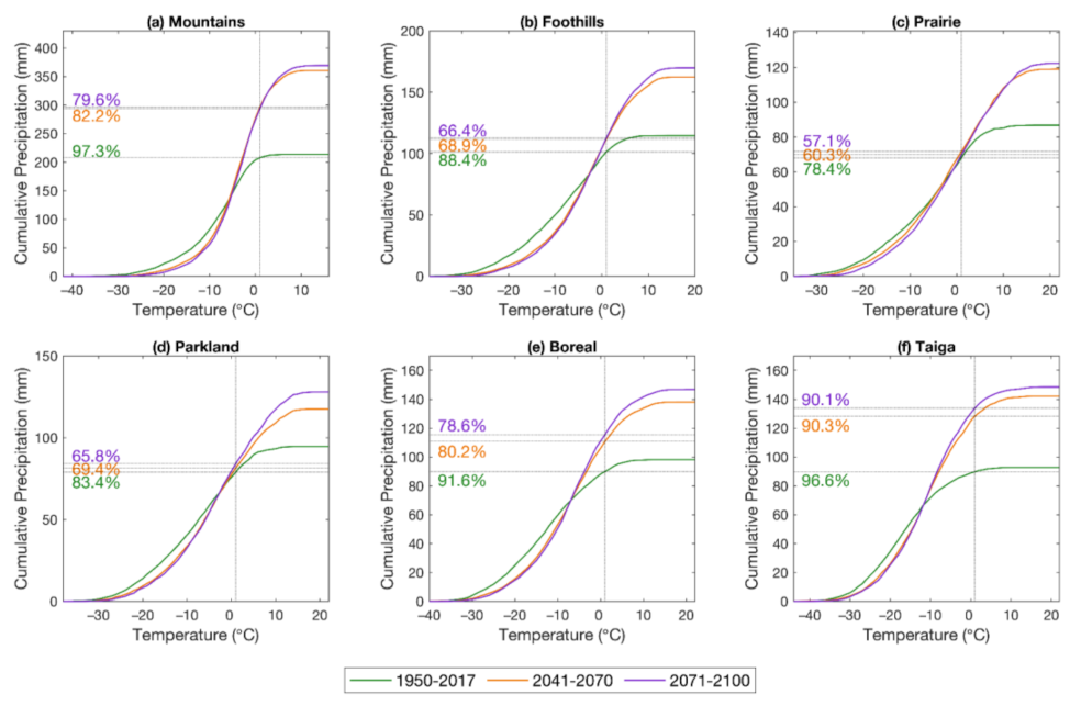
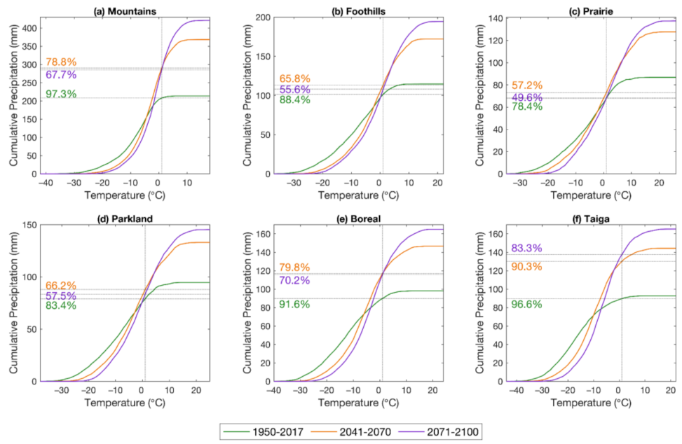
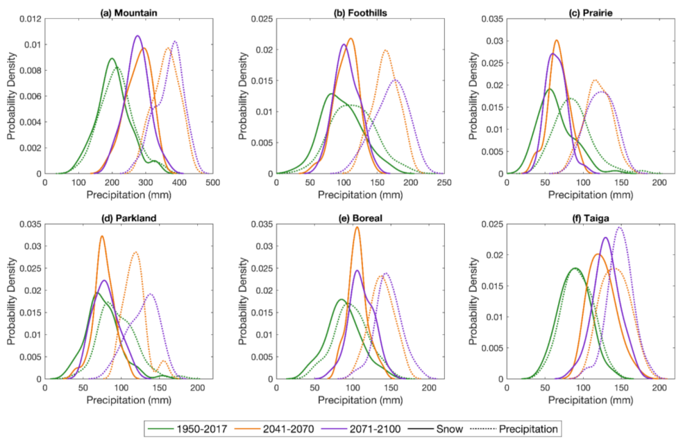
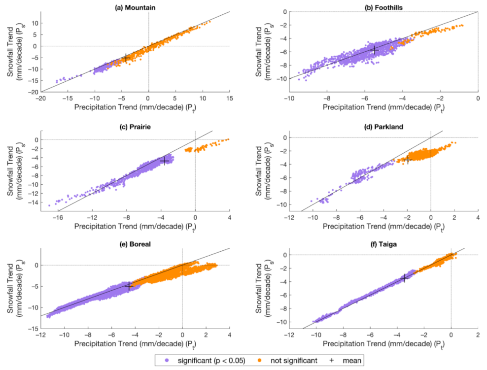
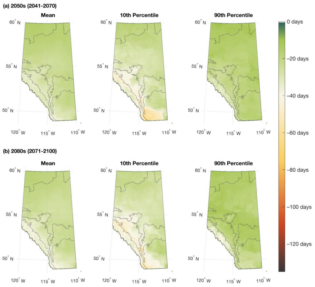
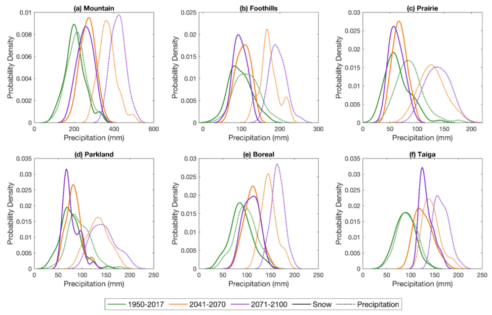
3.2.3. Winter Precipitation

Historic and future precipitation are given as cumulative distributions relative to mean daily temperature, and snowfall fraction, or percentage of total precipitation falling below the temperature threshold of 1 °C is indicated for each distribution. Total November–April precipitation is projected to increase substantially from the historic to 2050s and 2080s in all ecozones for RCP 4.5 (Figure 9) and RCP 8.5 (Figure 10). Cumulative precipitation below the 1 °C snow-rain threshold temperature is projected to increase for the Mountains, Boreal, and Taiga ecozones for both the 2050s and 2080s, and remain relatively stable for the Foothills, Prairie, and Parkland ecozones. For the Mountains, Boreal, and Taiga ecozones this indicates an increase in both rain and snow, suggesting gains in snowfall are offset by reductions in winter duration. Conversely, in the Foothills, Prairie, and Parkland ecozones, increases in precipitation are projected to fall as rain as a function of the attenuation of the winter season as well as changes in precipitation. There is little difference in projected cumulative precipitation amounts between the 2050s and 2080s for RCP 4.5 (Figure 9), while precipitation is projected to continue increasing through 2100 under RCP 8.5, such that the largest cumulative precipitation is seen for the 2080s for RCP 8.5 (Figure 10). Snowfall fraction has decreased for all ecozones for both RCP 4.5 and RCP 8.5 despite increases in snowfall for some of the ecozones, supporting indications that the projected increases in precipitation is largely in the form of rain. Notably, for the 2080s under RCP 8.5, less than 50% of total November–April precipitation in the Prairie ecozone is projected to fall as snow.
Precipitation–temperature distributions are projected to shift substantially for all future periods and RCP scenarios such that less precipitation is falling at lower temperatures and more precipitation at higher temperatures. This is particularly evident at the lower end of the temperature distribution where the historic cumulative precipitation lines lie above the distributions for both future periods and under RCP 4.5 and RCP 8.5 scenarios. For example, in the Boreal ecozone, approximately 60 mm of precipitation fell when the mean daily temperature was below −10 °C in the historic period, which is reduced to approximately 45 mm in the 2050s and 35 mm in the 2080s for RCP 8.5. This has implications for the temperature of the snowpack, and consequently, the vulnerability to snowmelt. A snowpack that is closer to 0 °C isothermal will melt faster than a cold snowpack as energy inputs to a cold snowpack (e.g., temperature, solar radiation) will first be used to raise the temperature of the snowpack to 0 °C before a phase change from solid to liquid can occur [21]. A shift in the distribution of precipitation with temperature suggests a warmer snowpack and thus less energy required to raise the temperature of a snowpack to initiate snowmelt.
Variability in November–April ecozone-averaged total precipitation and snowfall are given as probability density functions (PDFs) for RCP 4.5 (Figure 11) and RCP 8.5 (Figure 12). In the historic period, snow (solid line) and total precipitation (dotted line) appear fairly well coupled for all ecozones, consistent with cumulative precipitation plots indicating the majority of precipitation falls as snow. Conversely, future scenarios signify a decoupling of snowfall from total precipitation. Additionally, the variability of historic snowfall and total precipitation is greater than future scenarios, evident by the wider spread of the distribution curve and lower probabilities around the mean values compared with future distribution curves. This is particularly pronounced for snowfall in both RCP 4.5 (Figure 11) and RCP 8.5 (Figure 12) scenarios where snowfall PDFs are narrow and probabilities of near-mean values are high. Probability distributions of both snow and total precipitation are shifted such that historically high-probability average-precipitation values decrease in probability for future scenarios for Mountain, Boreal, and Taiga ecozones and increase in probability for Foothills, Prairie, and Parkland ecozones in both RCP 4.5 and RCP 8.5. Similarly, historically low-probability high-precipitation values in Mountain, Boreal, and Taiga are projected to increase in probability in future scenarios. For example, in the Mountain ecozone during the historic period, the cumulative snowfall probabilities peak ~200 mm and there is a low probability of 300 mm of snowfall, where in the 2050s under RCP 4.5, the probability of 300 mm of snowfall is nearly 10 times greater than the historic period, and the probability of 200 mm of snowfall is nearly 5 times lower.

4. Discussion

The results of this study show that the dynamics of cryosphere-related climate variables have changed since the mid-20th century and that future climate projections under two potential emissions scenarios indicate these changes are expected to accelerate over the 21st century; furthermore, this may have major implications for the spatial and temporal distribution of freshwater in western Canada. These changes represent the cumulative effect of increasing temperatures, shortening the duration of winter and advancing the onset of spring above-freezing temperatures, and shifting patterns of the amount and phase of cold season precipitation. The magnitude of projected shifts in temperature and precipitation metrics depend on emissions pathway, where a greater impact to snow accumulation and melt regimes is expected under RCP 8.5. While the historic period is characterized by a loss of cold season precipitation and a shift from snow to rain for most of Alberta, a reversal is projected for the 2050s and 2080s such that cold season precipitation is projected to increase, while continued decreases in winter duration are projected. This will potentially create novel winter climates not currently seen in these ecozones. Changes in precipitation, snow accumulation, and timing of snowmelt in the Mountain ecozone has implications for water resource availability for large downstream areas in western and northern Canada, while changes in all other ecozones has primarily local or regional impacts on runoff, groundwater recharge, agriculture, and ecosystem function.
Spatial and temporal gradients in the magnitude of historic trends and future projections exist among ecozones. In the historic period, the ecozones with the greatest change in the timing of the spring 0 °C isotherm and winter duration (Prairie and Parkland) saw the biggest divergence between winter snowfall and precipitation trends, indicating a shift from snow to rain in addition to a loss of precipitation. Conversely, ecozones with the lowest rate of change in temperature metrics (Taiga and Mountain) saw a roughly equal trend magnitude in both winter snowfall and precipitation. This demonstrates the importance of winter duration for snow accumulation. While the Mountain ecozone remained relatively stable with respect to climate metrics over the historic period, this ecozone emerges as a region of amplified vulnerability due to an attenuated winter duration and earlier onset of spring temperatures relative to other ecozones. Despite decreases in the snow accumulation season, substantial increases in precipitation and the amount of precipitation falling as snow are projected for both the 2050s and 2080s under both emissions scenarios, where the projected gains in precipitation in the Mountain ecozone is 2–3 times greater than other ecozones. These results indicate that future streamflow through the Plains will continue to be dominated by Mountain headwater contributions. However, given projected shifts in cold season temperature and precipitation patterns, mid-winter melt or rain on snow and earlier spring onset may alter the timing and magnitude of streamflow downstream.
Changes between historic and future climate variability indicate the potential for large deviations from the projected mean values, particularly for shifts in the 10th percentile of the distributions. Consequently, future scenarios include the potential for a very early onset of spring temperatures and an extremely short winter duration for all ecozones. Of particular concern are regions in southern and western Alberta that are projected to include winters that remain above freezing in future scenarios, including an area of the western Prairie ecozone where up to 21% of the years between 2071–2100 are projected to remain above freezing. This suggests that while discrete snowfall events may occur, it is unlikely snow will accumulate, which will affect soil freeze-thaw cycles, groundwater recharge and flow dynamics, and agricultural and natural ecosystems. Currently, in the southwestern Alberta prairie, winter temperature fluctuations above and below freezing, commonly related to warm Chinook winds descending the eastern slopes of the Rocky Mountains, result in oscillating periods of snowpack development and disappearance [81]. The projected shifts in winter duration and the timing of spring above-freezing temperatures suggest that this phenomena will likely be exacerbated in the future.
Cold season climate change is projected to decouple the probability distributions of total precipitation and snowfall as rising temperatures drive a shift from snow to rain. Furthermore, probabilities are projected to shift such that historically frequent seasonal precipitation and snowfall amounts may occur in the future, but at lower probabilities. Historically rare high precipitation amounts are projected to become more common and historically rare low precipitation amounts do not occur in future probability distributions. This creates new cold season precipitation regimes, the hydrologic impacts of which will vary depending on dominant catchment characteristics such as topography, subsurface storage dynamics, and land cover and use [82]. Rising temperatures are also projected to shift the range of temperatures at which precipitation falls in all ecozones, including a decrease in precipitation falling at lower temperatures, indicative of the potential for warmer snowpacks and increased vulnerability to melt [21].
Historic precipitation trends indicate that most ecozones have seen a decline in total precipitation and a shift from snow to rain and future scenarios all predict a decrease in snowfall fraction in tandem with increasing precipitation. Annual streamflow is positively related to the percentage of total precipitation that falls as snow [83,84]; therefore, a decrease in snowfall fraction is expected to elicit a nonlinear hydrologic response. Additionally, an earlier onset of spring temperatures may not result in a detectably earlier spring freshet as energy limitations during late winter and early spring attenuate snowmelt rates [22,25] or weaken relationships between snowpack and spring hydrology [26,27]. Spring runoff should be monitored and evaluated for changes in magnitude and climate-hydrologic coupling. Both snowmelt and rainfall are important drivers of groundwater recharge; therefore, shifts from snow to rain may not negatively impact recharge as long as total precipitation remains high [10]. However, an increase in the volume of seasonal precipitation and rising temperatures will likely alter water table and soil freezing depths in many ecozones, altering groundwater recharge and storage dynamics. In prairie regions, snowmelt that collects in topographic depressions melts and slowly infiltrates or is stored in surface ponding until soil thaws [85]. The depth and extent of frozen soil is a function of climate [86], and under climate warming, the dynamics of frozen ground may change [87,88], which can affect the snowmelt runoff ratio [89]. For example, midwinter melts are shown to refreeze in the subsurface and increase runoff during spring melt [90]. Therefore, increased precipitation may translate to greater groundwater recharge, storage, and runoff. Furthermore, groundwater recharge may be initiated earlier in the season or throughout the winter season under future climate conditions.
Increases in cold season precipitation may exacerbate mechanisms that increase the potential for flooding. For example, high soil moisture due to increased precipitation, inhibits further infiltration and leads to excess runoff [91]. In Mountain and Foothills ecozones, heavy precipitation events and/or rain on snow have contributed to major flooding events in southern Alberta [92,93]. Effective water management strategies throughout the watershed are necessary to mitigate flood impacts, e.g., [94]. Rain on snow is of particular concern as it can generate greater runoff than rain alone [19,95], and evidence indicates the frequency of rain on snow events will increase over mid- to high-elevations in the province [18]. While higher winter precipitation can exacerbate flood risk, earlier snowmelt is linked to lower summer streamflow [24] and can contribute to water deficits during the summer season. Despite projected increases in winter precipitation, widespread annual and summer water deficits, evaluated using the Standardized Precipitation-Evapotranspiration Index, are projected, particularly for southern Alberta [96,97]. Strong contrasting projections of winter and summer climate is expected to intensify oscillations between water surplus and deficits. Therefore, water management strategies may be necessary to ensure seasonal redistribution of water resources, while balancing socioeconomic and ecological requirements. Future research based holistically on annual cycles of water resource availability, with a particular focus on identifying transition periods between surplus and deficit and the evolving role of glacial melt in the annual water balance, will further inform adaptation strategies, water resource management, and environmental monitoring programs.
Results of this study are consistent with other evaluations of historic trends and future projections of cold season climate. Although results from both emissions scenarios are in agreement on the direction of projected changes, and are in agreement with other studies, e.g., [3,5,32], there is uncertainty over the magnitude of changes to the mean and variability of each climate metric. It is critical to continue evaluating future climate scenarios to refine our understanding of future impacts to climate and to evaluate the performance of existing projections as climate observations begin to overlap with projected future climatologies. Additionally, future research should investigate whether regional climate models (RCMs) could provide added value by improving the representation of regional climate simulated by the driving GCMs [98,99]. However, the added value by RCM simulations can be difficult to quantify [98,100], and depends on different factors such as scale, variable, region of interest, application, and experiment configuration [100]. Several recent studies have presented climate projections over a larger spatial scale, e.g., [3,28], or averaged over a watershed, e.g., [5,32]. While watershed-averaging provides valuable information for water availability, we know that mountain headwaters contribute a disproportionately large quantity of fresh water. At the provincial scale, evaluating historic trends and future projections by ecozone facilitates the understanding of regional variability of climate change and potential impacts at local scales, which is critical for making regional or sector-specific water management decisions [37]. Additionally, as the dominant source of streamflow, historic and projected changes in the Mountain ecozone informs large-scale water availability for several major rivers in western Canada.

5. Conclusions

Analyses of key winter temperature and precipitation metrics reveal considerable spatial and temporal variability in changes to snow accumulation and melt regimes over the historic period and projected over the 21st century. The historic period was dominated by trends toward an earlier onset of spring above-freezing temperatures, shorter winter duration, decreased precipitation coupled with a shift from snow to rain, especially in the Prairie and Parkland ecozones. The trajectory of the spring 0 °C isotherm and winter duration is projected to continue through the 21st century; however, the decreasing precipitation and snowfall trends seen over the historic period are expected to reverse and substantial increases are projected for future periods. The magnitude of projected changes are dependent on the emissions pathway, with more pronounced changes projected under a continued rise in emissions (RCP 8.5) compared with an emissions stabilization scenario (RCP 4.5).
Uneven rates of change, particularly in the Mountain ecozone, leads to changes in winter climate gradients among ecozones, which is expected to change the dynamics of snowmelt timing across the province. Projected changes in variability lead a heightened potential for an extremely early spring onset and short winter duration, with the Prairie ecozone emerging as a region vulnerable to loss of a sustained cold season. Projected changes in cold season precipitation and snowfall distributions decrease the potential for low precipitation and snowfall amounts while increasing the potential for high precipitation and snowfall.
Freshwater is important for maintaining ecosystem function in the six ecozones in Alberta and aquatic ecosystems in major rivers in western Canada. It is a major component of socioeconomic systems and traditional livelihoods in the province [39]. A temporal redistribution of water resources and substantial changes to the amounts of water availability pose a risk to these ecological, socioeconomic, and traditional needs. With strategic water management tools and decisions, the challenges presented by the changing patterns of precipitation and temperature can be faced to maintain water security in the future.

Supplementary Materials

The following are available online at https://www.mdpi.com/article/10.3390/w13081013/s1, Figure S1: Projected change in autumn 0 °C isotherm dates—mean, 10th percentile (earliest), and 90th percentile (latest) between the historic period (1950–2017) and (a) 2050s (2041–2070) and (b) 2080s (2071–2100) for RCP 4.5, Figure S2: Projected change in autumn 0 °C isotherm dates—mean, 10th percentile (earliest), and 90th percentile (latest) between the historic period (1950–2017) and (a) 2050s (2041–2070) and (b) 2080s (2071–2100) for RCP 8.5, Table S1: Average change in autumn 0 °C isotherm timing, given in as the change in the number of days between the historic baseline and future periods.

Author Contributions

Conceptualization, B.W.N. and J.F.O.; methodology, B.W.N. and B.F.; software, B.W.N. and B.F.; formal analysis, B.W.N.; data curation, B.W.N.; writing—original draft preparation, B.W.N. and B.F.; writing—review and editing, B.W.N., B.F. and J.F.O.; visualization, B.W.N. All authors have read and agreed to the published version of the manuscript.

Funding

This research received no external funding.

Institutional Review Board Statement

Not applicable.

Informed Consent Statement

Not applicable.

Data Availability Statement

No new data were created or analyzed in this study. Data sharing is not applicable to this article.

Acknowledgments

The authors gratefully acknowledge the two anonymous reviewers whose comments helped improve this manuscript.

Conflicts of Interest

The authors declare no conflict of interest.

References

  1. Viviroli, D.; Dürr, H.H.; Messerli, B.; Meybeck, M.; Weingartner, R. Mountains of the world, water towers for humanity: Typology, mapping, and global significance. Water Resour. Res. 2007, 43, W07447. [Google Scholar] [CrossRef] [Green Version]
  2. Derksen, C.; Burgess, D.; Duguay, C.; Howell, S.; Mudryk, L.; Smith, S.; Thackeray, C.; Kirchmeier-Young, M. Changes in snow, ice, and permafrost across Canada. In Canada’s Changing Climate Report; Bush, E., Lemmen, D.S., Eds.; Government of Canada: Ottawa, ON, Canada, 2018; pp. 194–260. [Google Scholar]
  3. Zhang, X.; Flato, G.; Kirchmeier-Young, M.; Vincent, L.; Wan, H.; Wang, X.; Rong, R.; Fyfe, J.; Li, G.; Kharin, V.V. Changes in Temperature and Precipitation Across Canada. In Canada’s Changing Climate Report; Bush, E., Lemmen, D.S., Eds.; Government of Canada: Ottawa, ON, Canada, 2019; pp. 112–193. [Google Scholar]
  4. Bonsal, B.; Peters, D.L.; Seglenieks, F.; Rivera, A.; Berg, A. Changes in freshwater availability across Canada. In Canada’s Changing Climate Report; Bush, E., Lemmen, D.S., Eds.; Government of Canada: Ottawa, ON, Canada, 2019; pp. 261–342. [Google Scholar]
  5. Bonsal, B.; Shrestha, R.R.; Dibike, Y.; Peters, D.L.; Spence, C.; Mudryk, L.; Yang, D. Western Canadian freshwater availability: Current and future vulnerabilities. Environ. Rev. 2020, 28, 528–545. [Google Scholar] [CrossRef]
  6. Barnett, T.P.; Adam, J.C.; Lettenmaier, D.P. Potential impacts of a warming climate on water availability in snow-dominated regions. Nature 2005, 438, 303–309. [Google Scholar] [CrossRef]
  7. Immerzeel, W.W.; Lutz, A.F.; Andrade, M.; Bahl, A.; Biemans, H.; Bolch, T.; Hyde, S.; Brumby, S.; Davies, B.J.; Elmore, A.C.; et al. Importance and vulnerability of the world’s water towers. Nature 2020, 577, 364–369. [Google Scholar] [CrossRef]
  8. Wrona, F.J.; Johansson, M.; Culp, J.M.; Jenkins, A.; Mård, J.; Myers-Smith, I.H.; Prowse, T.; Vincent, W.F.; Wookey, P.A. Transitions in Arctic ecosystems: Ecological implications of a changing hydrological regime. J. Geophys. Res. Biogeosci. 2016, 121, 650–674. [Google Scholar] [CrossRef] [Green Version]
  9. Redding, T.; Devito, K. Aspect and soil textural controls on snowmelt runoff on forested Boreal Plain hillslopes. Hydrol. Res. 2011, 42, 250–267. [Google Scholar] [CrossRef]
  10. Hayashi, M.; Farrow, C.R. Watershed-scale response of groundwater recharge to inter-annual and inter-decadal variability in precipitation (Alberta, Canada). Hydrogeol. J. 2014, 22, 1825–1839. [Google Scholar] [CrossRef]
  11. Fang, X.; Pomeroy, J.W. Modelling blowing snow redistribution to prairie wetlands. Hydrol. Process. 2009, 23, 2557–2569. [Google Scholar] [CrossRef]
  12. Hayashi, M.; van der Kamp, G.; Rosenberry, D.O. Hydrology of prairie wetlands: Understanding the integrated surface-water and groundwater processes. Wetlands 2016, 36, 237–254. [Google Scholar] [CrossRef]
  13. Moore, R.D.; Demuth, M.N. Mass balance and streamflow variability at Place Glacier, Canada, in relation to recent climate fluctuations. Hydrol. Process. 2001, 15, 3473–3486. [Google Scholar] [CrossRef]
  14. Hamlet, A.F.; Mote, P.W.; Clark, M.P.; Lettenmaier, D.P. Effects of temperature and precipitation variability on snowpack trends in the western United States. J. Clim. 2005, 18, 4545–4561. [Google Scholar] [CrossRef]
  15. Nolin, A.W.; Daly, C. Mapping “at risk” snow in the Pacific Northwest. J. Hydrometeorol. 2006, 7, 1164–1171. [Google Scholar] [CrossRef]
  16. Adam, J.C.; Hamlet, A.F.; Lettenmaier, D.P. Implications of global climate change for snowmelt hydrology in the twenty-first century. Hydrol. Process. 2009, 23, 962–972. [Google Scholar] [CrossRef]
  17. Lundquist, J.D.; Neiman, P.J.; Martner, B.; White, A.B.; Gottas, D.J.; Ralph, F.M. Rain versus snow in the Sierra Nevada, California: Comparing Doppler profiling radar and surface observations of melting level. J. Hydrometeorol. 2008, 9, 194–211. [Google Scholar] [CrossRef] [Green Version]
  18. Musselman, K.N.; Lehner, F.; Ikeda, K.; Clark, M.P.; Prein, A.F.; Liu, C.; Barlage, M.; Rasmussen, R. Projected increases and shifts in rain-on-snow flood risk over western North America. Nat. Clim. Chang. 2018, 8, 808–812. [Google Scholar] [CrossRef]
  19. Marks, D.; Kimball, J.; Tingey, D.; Link, T. The sensitivity of snowmelt processes to climate conditions and forest cover during rain-on-snow: A case study of the 1996 Pacific Northwest flood. Hydrol. Process. 1998, 12, 1569–1587. [Google Scholar] [CrossRef]
  20. Sui, J.; Koehler, G. Rain-on-snow induced flood events in Southern Germany. J. Hydrol. 2001, 252, 205–220. [Google Scholar] [CrossRef]
  21. U.S. Army Corps of Engineers. Snow Hydrology: Summary Report of the Snow Investigations; North Pacific Division: Portland, OR, USA, 1956; pp. 1–437. [Google Scholar]
  22. Musselman, K.N.; Clark, M.P.; Liu, C.; Ikeda, K. Slower snowmelt in a warmer world. Nat. Clim. Chang. 2017, 7, 214–219. [Google Scholar] [CrossRef]
  23. Abdul Aziz, O.I.A.; Burn, D.H. Trends and variability in the hydrological regime of the Mackenzie River Basin. J. Hydrol. 2006, 319, 282–294. [Google Scholar] [CrossRef]
  24. Rood, S.B.; Pan, J.; Gill, K.M.; Franks, C.G.; Samuelson, G.M.; Shepherd, A. Declining summer flows of Rocky Mountain rivers: Changing seasonal hydrology and probable impacts on floodplain forests. J. Hydrol. 2008, 349, 397–410. [Google Scholar] [CrossRef]
  25. Barnhart, T.B.; Tague, C.L.; Molotch, N.P. The counteracting effects of snowmelt rate and timing on runoff. Water Resour. Res. 2020, 56, e2019WR026634. [Google Scholar] [CrossRef]
  26. López-Moreno, I.; Pomeroy, J.W.; Alonso-González, E.; Morán-Tejeda, E.; Revuelto-Benedí, J. Decoupling of warming mountain snowpacks from hydrological regimes. Environ. Res. Lett. 2020, 15, 114006. [Google Scholar] [CrossRef]
  27. Grogan, D.S.; Burakowski, E.A.; Contosta, A.R. Snowmelt control on spring hydrology declines as the vernal window lengthens. Environ. Res. Lett. 2020, 15, 114040. [Google Scholar] [CrossRef]
  28. Collins, M.; Knutti, R.; Arblaster, J.; Dufresne, J.-L.; Fichefet, T.; Friedlingstein, P.; Gao, X.; Gutowski, W.J.; Johns, T.; Krinner, G.; et al. Long-term Climate Change: Projections, Commitments and Irreversibility. In Climate Change 2013: The Physical Science Basis. Contribution of Working Group I to the Fifth Assessment Report of the Intergovernmental Panel on Climate Change; Stocker, T.F., Qin, D., Plattner, G.-K., Tignor, M., Allen, S.K., Boschung, J., Nauels, A., Xia, Y., Bex, V., Midgley, P.M., Eds.; Cambridge University Press: Cambridge, UK; New York, NY, USA, 2013; pp. 1029–1136. [Google Scholar]
  29. Vincent, L.A.; Zhang, X.; Brown, R.D.; Feng, Y.; Mekis, É.; Milewska, E.J.; Wan, H.; Wang, X.L. Observed trends in Canada’s climate and influence of low-frequency variability modes. J. Clim. 2015, 28, 4545–4560. [Google Scholar] [CrossRef]
  30. O’Neil, H.C.L.; Prowse, T.D.; Bonsal, B.R.; Dibike, Y.B. Spatial and temporal characteristics in streamflow-related hydroclimatic variables over western Canada. Part 1: 1950–2010. Hydrol. Res. 2017, 48, 915–931. [Google Scholar] [CrossRef]
  31. Kienzle, S.W. Has it become warmer in Alberta? Mapping temperature changes for the period 1950–2010 across Alberta, Canada. Can. Geogr. 2018, 62, 144–162. [Google Scholar] [CrossRef]
  32. O’Neil, H.C.L.; Prowse, T.D.; Bonsal, B.R.; Dibike, Y.B. Spatial and temporal characteristics in streamflow-related hydroclimatic variables over western Canada. Part 2: Future projections. Hydrol. Res. 2017, 48, 932–944. [Google Scholar] [CrossRef]
  33. Mekis, É.; Vincent, L.A. An overview of the second generation adjusted daily precipitation dataset for trend analysis in Canada. Atmos. Ocean 2011, 49, 163–177. [Google Scholar] [CrossRef] [Green Version]
  34. Vincent, L.A.; Zhang, X.; Mekis, É.; Wan, H.; Bush, E.J. Changes in Canada’s climate: Trends in indices based on daily temperature and precipitation data. Atmos. Ocean 2018, 56, 332–349. [Google Scholar] [CrossRef] [Green Version]
  35. Brown, R.D.; Fang, B.; Mudryk, L. Update of Canadian historical snow survey data and analysis of snow water equivalent trends, 1967–2016. Atmos. Ocean 2019, 57, 149–156. [Google Scholar] [CrossRef]
  36. Mudryk, L.R.; Derksen, C.; Howell, S.; Laliberté, F.; Thackeray, C.; Sospedra-Alfonso, R.; Vionnet, V.; Kushner, P.J.; Brown, R. Canadian snow and sea ice: Historical trends and projections. Cryosphere 2018, 12, 1157–1176. [Google Scholar] [CrossRef] [Green Version]
  37. Haine, T.W.; Curry, B.; Gerdes, R.; Hansen, E.; Karcher, M.; Lee, C.; Rudels, B.; Spreen, G.; de Steur, L.; Stewart, K.D.; et al. Arctic freshwater export: Status, mechanisms, and prospects. Glob. Planet. Chang. 2015, 125, 13–35. [Google Scholar] [CrossRef] [Green Version]
  38. Carmack, E.C.; Yamamoto-Kawai, M.; Haine, T.W.; Bacon, S.; Bluhm, B.A.; Lique, C.; Melling, H.; Polyakov, I.V.; Straneo, F.; Timmermans, M.-L.; et al. Freshwater and its role in the Arctic Marine System: Sources, disposition, storage, export, and physical and biogeochemical consequences in the Arctic and global oceans. J. Geophys. Res. Biogeosci. 2016, 121, 675–717. [Google Scholar] [CrossRef]
  39. Alberta Environment and Parks. Knowledge for a Changing Environment: 2019–2024 Science Strategy. 2019. Available online: open.alberta.ca/publications/9781460142370 (accessed on 13 December 2019).
  40. Ecological Stratification Working Group. A National Ecological Framework for Canada; Agriculture and Agri-Food Canada, Research Branch, Centre for Land and Biological Resources Research and Environment Canada, State of Environment Directorate: Ottawa, ON, Canada; Hull, QC, Canada, 1996; pp. 1–125. [Google Scholar]
  41. van der Kamp, G.; Hayashi, M. Groundwater-wetland ecosystem interaction in the semiarid glaciated plains of North America. Hydrogeol. J. 2009, 17, 203–214. [Google Scholar] [CrossRef]
  42. Hutchinson, M.F.; McKenney, D.W.; Lawrence, K.; Pedlar, J.H.; Hopkinson, R.F.; Milewska, E.; Papadopol, P. Development and testing of Canada-wide interpolated spatial models of daily minimum–maximum temperature and precipitation for 1961–2003. J. Appl. Meteorol. Clim. 2009, 48, 725–741. [Google Scholar] [CrossRef]
  43. McKenney, D.W.; Hutchinson, M.F.; Papadopol, P.; Lawrence, K.; Pedlar, J.; Campbell, K.; Milewska, E.; Hopkinson, R.F.; Price, D.; Owen, T. Customized spatial climate models for North America. Bull. Am. Meteorol. Soc. 2011, 92, 1611–1622. [Google Scholar] [CrossRef]
  44. Hopkinson, R.F.; McKenney, D.W.; Milewska, E.J.; Hutchinson, M.F.; Papadopol, P.; Vincent, L.A. Impact of aligning climatological day on gridding daily maximum–minimum temperature and precipitation over Canada. J. Appl. Meteorol. Clim. 2011, 50, 1654–1665. [Google Scholar] [CrossRef]
  45. Bonsal, B.R.; Aider, R.; Gachon, P.; Lapp, S. An assessment of Canadian prairie drought: Past, present, and future. Clim. Dyn. 2013, 41, 501–516. [Google Scholar] [CrossRef]
  46. Newton, B.W.; Prowse, T.D.; Bonsal, B.R. Evaluating the distribution of water resources in western Canada using synoptic climatology and selected teleconnections. Part 1: Winter season. Hydrol. Process. 2014, 28, 4219–4234. [Google Scholar] [CrossRef]
  47. Curry, C.L.; Tencer, B.; Whan, K.; Weaver, A.J.; Giguère, M.; Wiebe, E. Searching for added value in simulating climate extremes with a high-resolution regional climate model over western Canada. Atmos. Ocean 2016, 54, 364–384. [Google Scholar] [CrossRef]
  48. Islam, S.U.; Déry, S.J. Evaluating uncertainties in modelling the snow hydrology of the Fraser River Basin, British Columbia, Canada. Hydrol. Earth Syst. Sci. 2017, 21, 1827–1847. [Google Scholar] [CrossRef] [Green Version]
  49. Eum, H.I.; Dibike, Y.; Prowse, T. Climate-induced alteration of hydrologic indicators in the Athabasca River Basin, Alberta, Canada. J. Hydrol. 2017, 544, 327–342. [Google Scholar] [CrossRef]
  50. Sobie, S.R.; Murdock, T.Q. High-resolution statistical downscaling in southwestern British Columbia. J. Appl. Meteorol. Clim. 2017, 56, 1625–1641. [Google Scholar] [CrossRef]
  51. Werner, A.T.; Cannon, A.J. Hydrologic extremes—An intercomparison of multiple gridded statistical downscaling methods. Hydrol. Earth Syst. Sci. 2016, 20, 1483–1508. [Google Scholar] [CrossRef] [Green Version]
  52. Stahl, K.; Moore, R.D.; Floyer, J.A.; Asplin, M.G.; McKendry, I.G. Comparison of approaches for spatial interpolation of daily air temperature in a large region with complex topography and highly variable station density. Agric. Forest Meteorol. 2006, 139, 224–236. [Google Scholar] [CrossRef]
  53. Eum, H.I.; Dibike, Y.; Prowse, T.; Bonsal, B. Inter-comparison of high-resolution gridded climate data sets and their implication on hydrological model simulation over the Athabasca Watershed, Canada. Hydrol. Process. 2014, 28, 4250–4271. [Google Scholar] [CrossRef]
  54. Singh, H.; Najafi, M.R. Evaluation of gridded climate datasets over Canada using univariate and bivariate approaches: Implications for hydrological modelling. J. Hydrol. 2020, 584, 124673. [Google Scholar] [CrossRef]
  55. Wong, J.S.; Razavi, S.; Bonsal, B.R.; Wheater, H.S.; Asong, Z.E. Inter-comparison of daily precipitation products for large-scale hydro-climatic applications over Canada. Hydrol. Earth Syst. Sci. 2017, 21, 2163–2185. [Google Scholar] [CrossRef] [Green Version]
  56. Myhre, G.; Shindell, D.; Bréon, F.-M.; Collins, W.; Fuglestvedt, J.; Huang, J.; Koch, D.; Lamarque, J.-F.; Lee, D.; Mendoza, B.; et al. Anthropogenic and Natural Radiative Forcing. In Climate Change 2013: The Physical Science Basis. Contribution of Working Group I to the Fifth Assessment Report of the Intergovernmental Panel on Climate Change; Stocker, T.F., Qin, D., Plattner, G.-K., Tignor, M., Allen, S.K., Boschung, J., Nauels, A., Xia, Y., Bex, V., Midgley, P.M., Eds.; Cambridge University Press: Cambridge, UK; New York, NY, USA, 2013; pp. 659–740. [Google Scholar]
  57. Barrow, E.; Yu, G.E. Climate Scenarios for Alberta; Prairie Adaptation Research Collaborative: Regina, SK, Canada, 2005; pp. 1–73. [Google Scholar]
  58. Cannon, A.J. Selecting GCM scenarios that span the range of changes in a multimodel ensemble: Application to CMIP5 climate extremes indices. J. Clim. 2015, 28, 1260–1267. [Google Scholar] [CrossRef]
  59. Farjad, B.; Gupta, A.; Sartipizadeh, H.; Cannon, A.J. A novel approach for selecting extreme climate change scenarios for climate change impact studies. Sci. Total Environ. 2019, 678, 476–485. [Google Scholar] [CrossRef] [PubMed]
  60. Lutz, A.F.; ter Maat, H.W.; Biemans, H.; Shrestha, A.B.; Wester, P.; Immerzeel, W.W. Selecting representative climate models for climate change impact studies: An advanced envelope-based selection approach. Int. J. Clim. 2016, 36, 3988–4005. [Google Scholar] [CrossRef] [Green Version]
  61. Sartipizadeh, H.; Vincent, T.L. Computing the approximate convex hull in high dimensions. arXiv 2016, arXiv:1603.04422. [Google Scholar]
  62. Pacific Climate Impacts Consortium, University of Victoria. Statistically Downscaled Climate Scenarios. Available online: https://data.pacificclimate.org/portal/downscaled_gcms/map/ (accessed on 11 May 2020).
  63. Mott, R.; Schirmer, M.; Bavay, M.; Grünewald, T.; Lehning, M. Understanding snow-transport processes shaping the mountain snow-cover. Cryosphere 2010, 4, 545–559. [Google Scholar] [CrossRef] [Green Version]
  64. Bernhardt, M.; Schulz, K.; Liston, G.E.; Zängl, G. The influence of lateral snow redistribution processes on snow melt and sublimation in alpine regions. J. Hydrol. 2012, 424, 196–206. [Google Scholar] [CrossRef]
  65. Bonsal, B.R.; Prowse, T.D. Trends and variability in spring and autumn 0 °C-isotherm dates over Canada. Clim. Chang. 2003, 57, 341–358. [Google Scholar] [CrossRef]
  66. Mann, H.B. Nonparametric tests against trend. Econometrica 1945, 13, 245–259. [Google Scholar] [CrossRef]
  67. Kendall, M.G. Rank Correlation Measures; Charles Griffin: London, UK, 1975. [Google Scholar]
  68. Sen, P.K. Estimates of the regression coefficient based on Kendall’s tau. J. Am. Stat. Assoc. 1968, 63, 1379–1389. [Google Scholar] [CrossRef]
  69. Bawden, A.J.; Linton, H.C.; Burn, D.H.; Prowse, T.D. A spatiotemporal analysis of hydrological trends and variability in the Athabasca River region, Canada. J. Hydrol. 2014, 509, 333–342. [Google Scholar] [CrossRef]
  70. Rood, S.B.; Kaluthota, S.; Philipsen, L.J.; Rood, N.J.; Zanewich, K.P. Increasing discharge from the Mackenzie River system to the Arctic Ocean. Hydrol. Process. 2017, 31, 150–160. [Google Scholar] [CrossRef]
  71. Bayazit, M.; Önöz, B. To prewhiten or not to prewhiten in trend analysis? Hydrolog Sci. J. 2007, 52, 611–624. [Google Scholar] [CrossRef]
  72. DeWalle, D.R.; Rango, A. Principles of Snow Hydrology; Cambridge University Press: Cambridge, UK, 2008. [Google Scholar]
  73. Harpold, A.A.; Kaplan, M.L.; Klos, P.Z.; Link, T.; McNamara, J.P.; Rajagopal, S.; Schumer, R.; Steele, C.M. Rain or snow: Hydrologic processes, observations, prediction, and research needs. Hydrol. Earth Syst. Sci. 2017, 21, 1–22. [Google Scholar] [CrossRef] [Green Version]
  74. Feiccabrino, J.; Lundberg, A.; Gustafsson, D. Improving surface-based precipitation phase determination through air mass boundary identification. Hydrol. Res. 2012, 43, 179–191. [Google Scholar] [CrossRef] [Green Version]
  75. Kienzle, S.W. A new temperature based method to separate rain and snow. Hydrol. Process. 2008, 22, 5067–5085. [Google Scholar] [CrossRef]
  76. Jennings, K.S.; Winchell, T.S.; Livneh, B.; Molotch, N.P. Spatial variation of the rain–snow temperature threshold across the Northern Hemisphere. Nat. Commun. 2018, 9, 1–9. [Google Scholar] [CrossRef] [Green Version]
  77. Feiccabrino, J.; Gustafsson, D.; Lundberg, A. Surface-based precipitation phase determination methods in hydrological models. Hydrol. Res. 2013, 44, 44–57. [Google Scholar] [CrossRef]
  78. Rohrer, M. Determination of the transition air temperature from snow to rain and intensity of precipitation. In WMO IASH ETH International Workshop on Precipitation Measurement; World Meteorological Organization: Geneva, Switzerland, 1989; pp. 475–582. [Google Scholar]
  79. L’hôte, Y.; Chevallier, P.; Coudrain, A.; Lejeune, Y.; Etchevers, P. Relationship between precipitation phase and air temperature: Comparison between the Bolivian Andes and the Swiss Alps. Hydrolog. Sci. J. 2005, 50, 989–997. [Google Scholar] [CrossRef]
  80. Newton, B.W.; Bonsal, B.R.; Edwards, T.W.; Prowse, T.D.; McGregor, G.R. Atmospheric drivers of winter above-freezing temperatures and associated rainfall in western Canada. Int. J. Climatol. 2019, 39, 5655–5671. [Google Scholar] [CrossRef]
  81. Pavlovskii, I.; Hayashi, M.; Itenfisu, D. Midwinter melts in the Canadian prairies: Energy balance and hydrological effects. Hydrol. Earth Syst. Sci. 2019, 23, 1867–1883. [Google Scholar] [CrossRef] [Green Version]
  82. Devito, K.J.; Creed, I.F.; Fraser, C.J.D. Controls on runoff from a partially harvested aspen-forested headwater catchment, Boreal Plain, Canada. Hydrol. Process. 2005, 19, 3–25. [Google Scholar] [CrossRef]
  83. Berghuijs, W.R.; Woods, R.A.; Hrachowitz, M. A precipitation shift from snow towards rain leads to a decrease in streamflow. Nat. Clim. Chang. 2014, 4, 583–586. [Google Scholar] [CrossRef] [Green Version]
  84. Hammond, J.C.; Harpold, A.A.; Weiss, S.; Kampf, S.K. Partitioning snowmelt and rainfall in the critical zone: Effects of climate type and soil properties. Hydrol. Earth Syst. Sci. 2019, 23, 3553–3570. [Google Scholar] [CrossRef] [Green Version]
  85. Hayashi, M.; van der Kamp, G.; Schmidt, R. Focused infiltration of snowmelt water in partially frozen soil under small depressions. J. Hydrol. 2003, 270, 214–229. [Google Scholar] [CrossRef]
  86. Shook, K.; Pomeroy, J.; van der Kamp, G. The transformation of frequency distributions of winter precipitation to spring streamflow probabilities in cold regions; case studies from the Canadian Prairies. J. Hydrol. 2015, 521, 395–409. [Google Scholar] [CrossRef]
  87. Qin, Y.; Yang, D.; Gao, B.; Wang, T.; Chen, J.; Chen, Y.; Wang, Y.; Zheng, G. Impacts of climate warming on the frozen ground and eco-hydrology in the Yellow River source region, China. Sci. Total Environ. 2017, 605, 830–841. [Google Scholar] [CrossRef] [Green Version]
  88. Frauenfeld, O.W.; Zhang, T. An observational 71-year history of seasonally frozen ground changes in the Eurasian high latitudes. Environ. Res. Lett. 2011, 6, 044024. [Google Scholar] [CrossRef] [Green Version]
  89. Koren, V.; Schaake, J.; Mitchell, K.; Duan, Q.Y.; Chen, F.; Baker, J.M. A parameterization of snowpack and frozen ground intended for NCEP weather and climate models. J. Geophys. Res. Atmos. 1999, 104, 19569–19585. [Google Scholar] [CrossRef]
  90. Mohammed, A.A.; Pavlovskii, I.; Cey, E.E.; Hayashi, M. Effects of preferential flow on snowmelt partitioning and groundwater recharge in frozen soils. Hydrol. Earth Syst. Sci. 2019, 23, 5017–5031. [Google Scholar] [CrossRef] [Green Version]
  91. Shook, K. The 2005 flood events in the Saskatchewan River Basin: Causes, assessment and damages. Can. Water Resour. J. 2016, 41, 94–104. [Google Scholar] [CrossRef]
  92. Liu, A.Q.; Mooney, C.; Szeto, K.; Thériault, J.M.; Kochtubajda, B.; Stewart, R.E.; Boodoo, S.; Goodson, R.; Li, Y.; Pomeroy, J. The June 2013 Alberta catastrophic flooding event: Part 1—Climatological aspects and hydrometeorological features. Hydrol. Process. 2016, 30, 4899–4916. [Google Scholar] [CrossRef] [Green Version]
  93. Pomeroy, J.W.; Fang, X.; Marks, D.G. The cold rain-on-snow event of June 2013 in the Canadian Rockies—Characteristics and diagnosis. Hydrol. Process. 2016, 30, 2899–2914. [Google Scholar] [CrossRef]
  94. Shook, K.; Pomeroy, J.W. The effects of the management of Lake Diefenbaker on downstream flooding. Can. Water Resour. J. 2016, 41, 261–272. [Google Scholar] [CrossRef]
  95. Garvelmann, J.; Pohl, S.; Weiler, M. Spatio-temporal controls of snowmelt and runoff generation during rain-on-snow events in a mid-latitude mountain catchment. Hydrol. Process. 2015, 29, 3649–3664. [Google Scholar] [CrossRef]
  96. Dibike, Y.; Prowse, T.; Bonsal, B.; O’Neil, H. Implications of future climate on water availability in the western Canadian river basins. Int. J. Climatol. 2017, 37, 3247–3263. [Google Scholar] [CrossRef]
  97. Tam, B.Y.; Szeto, K.; Bonsal, B.; Flato, G.; Cannon, A.J.; Rong, R. CMIP5 drought projections in Canada based on the Standardized Precipitation Evapotranspiration Index. Can. Water Resour. J. 2019, 44, 90–107. [Google Scholar] [CrossRef]
  98. Eden, J.M.; Widmann, M.; Maraun, D.; Vrac, M. Comparison of GCM-and RCM-simulated precipitation following stochastic postprocessing. J. Geophys. Res. Atmos. 2014, 119, 11040–11053. [Google Scholar] [CrossRef] [Green Version]
  99. Troin, M.; Caya, D.; Velázquez, J.A.; Brissette, F. Hydrological response to dynamical downscaling of climate model outputs: A case study for western and eastern snowmelt-dominated Canada catchments. J. Hydrol. Reg. Stud. 2015, 4, 595–610. [Google Scholar] [CrossRef] [Green Version]
  100. Torma, C.; Giorgi, F.; Coppola, E. Added value of regional climate modeling over areas characterized by complex terrain—Precipitation over the Alps. J. Geophys. Res. Atmos. 2015, 120, 3957–3972. [Google Scholar] [CrossRef]
Figure 1. Six ecozones in Alberta—Mountain, Foothills, Prairie, Parkland, Boreal, and Taiga.
Water 13 01013 g001
Figure 2. Trends (days/decade) in (a) spring 0 °C isotherm dates and (b) winter duration over the historic period (1950–2017). Only trends significant at p < 0.05 are shown.
Water 13 01013 g002
Figure 3. Trends in total November–April precipitation (x-axis) and precipitation falling as snow (y-axis) as determined through a temperature index rain–snow equation over the historic period (1950–2017). Points on the graphs represent ANUSPLIN grid points, at ~10 km resolution, within each ecozones and ecozone-averaged trends are indicated by a black plus sign (+). Reference lines represent equal precipitation and snowfall trend magnitude (Pt = Ps).
Water 13 01013 g003
Figure 4. Projected change in spring 0 °C isotherm dates—mean, 10th percentile (earliest), and 90th percentile (latest) between the historic period (1950–2017) and (a) 2050s (2041–2070) and (b) 2080s (2071–2100) for RCP 4.5.
Water 13 01013 g004
Figure 5. Projected change in spring 0 °C isotherm dates—mean, 10th percentile (earliest), and 90th percentile (latest) between the historic period (1950–2017) and (a) 2050s (2041–2070) and (b) 2080s (2071–2100) for RCP 8.5.
Water 13 01013 g005
Figure 6. Projected change in winter duration—mean, 10th percentile (earliest), and 90th percentile (latest) between the historic period (1950–2017) and (a) 2050s (2041–2070) and (b) 2080s (2071–2100) for RCP 4.5.
Water 13 01013 g006
Figure 7. Projected change in winter duration—mean, 10th percentile (earliest), and 90th percentile (latest) between the historic period (1950–2017) and (a) 2050s (2041–2070) and (b) 2080s (2071–2100) for RCP 8.5.
Water 13 01013 g007
Figure 8. Percentage of winters projected to remain above freezing, where no autumn or spring 0 °C isotherm is detected.
Water 13 01013 g008
Figure 9. Cumulative precipitation by temperature distribution for RCP 4.5. Snowfall fraction is shown as a percentage of total precipitation along the left side of each ecozone graph.
Water 13 01013 g009
Figure 10. Cumulative precipitation by temperature distribution for RCP 8.5. Snowfall fraction is shown as a percentage of total precipitation along the left side of each ecozone graph.
Water 13 01013 g010
Figure 11. Probability density function of total November–April snowfall (solid lines) and precipitation (dotted lines) amounts for historic and projected future periods under RCP 4.5.
Water 13 01013 g011
Figure 12. Probability density function of total November–April snowfall (solid lines) and precipitation (dotted lines) amounts for historic and projected future periods under RCP 8.5.
Water 13 01013 g012
Table 1. Area, elevation, and mean cold season (November–April) climate (1950–2017) for the six ecozones.
EcozoneArea (km2)Elevation Range and Mean (m.a.s.l.)Mean Cold Season Precipitation (mm)Mean Cold Season Temperature (°C)
Mountain47,000860–3630 (1890)214−0.5
Foothills68,000600–2450 (1060)1151.8
Prairie97,000590–1710 (880)874.2
Parkland59,000510–2010 (770)952.6
Boreal319,000160–1230 (560)980.4
Taiga72,000190–1000 (480)93−2.2
Table 2. List of initial pool of climate models used in this study.
ModelInstitutionCountry of Origin
BCC-CSM1Beijing Climate Center, China Meteorological AdministrationChina
BNU-ESMBeijing Normal UniversityChina
CanESM2Canadian Centre for Climate Modelling and AnalysisCanada
ACCESS-1.0Australian Community Climate and Earth-System Simulator-Bureau’s Research and Development BranchAustralia
IPSL-CM5A-MRInstitut Pierre Simon LaplaceFrance
IPSL-CM5A-LRInstitut Pierre Simon LaplaceFrance
MIROC5Center for Climate System Research (University of Tokyo), National Institute for Environmental Studies, and Frontier Research Center for Global ChangeJapan
MIROC-ESMCenter for Climate System Research (University of Tokyo), National Institute for Environmental Studies, and Frontier Research Center for Global ChangeJapan
MIROC-CHEMCenter for Climate System Research (University of Tokyo), National Institute for Environmental Studies, and Frontier Research Center for Global ChangeJapan
MPI-ESM-LRMax Planck Institute for MeteorologyGermany
MPI-ESM-MRMax Planck Institute for MeteorologyGermany
CCSM4National Center for Atmospheric ResearchUSA
HadGEM2-ESHadley Centre for Climate Prediction and ResearchUK
HadGEM2-CCHadley Centre for Climate Prediction and ResearchUK
CNRM-CM5Météo-France/Centre National de Recherches MétéorologiquesFrance
CSIRO-Mk3-6-0Commonwealth Scientific and Industrial Research Organisation (CSIRO) Atmospheric ResearchAustralia
GFDL-CM3National Oceanic and Atmospheric Administration (NOAA)/Geophysical Fluid Dynamics LaboratoryUSA
GFDL-ESM2GNational Oceanic and Atmospheric Administration (NOAA)/Geophysical Fluid Dynamics LaboratoryUSA
GFDL- ESM2MNational Oceanic and Atmospheric Administration (NOAA)/Geophysical Fluid Dynamics LaboratoryUSA
INMCM4Institute for Numerical Mathematics, RussiaRussia
MRI-CGCM3Meteorological Research InstituteJapan
CESM1-BGCCommunity Earth System Model- National Science Foundation (NSF) and the U.S. Department of Energy (DOE)USA
CMCC-CMEuro-Mediterranean Center on Climate ChangeItaly
FGOALS-g2National Key Laboratory of Numerical Modeling for Atmospheric Sciences and Geophysical Fluid Dynamics (LASG)/Institute of Atmospheric PhysicsChina
FGOALS-s2National Key Laboratory of Numerical Modeling for Atmospheric Sciences and Geophysical Fluid Dynamics (LASG)/Institute of Atmospheric PhysicsChina
NorESM1-MNorwegian Climate Centre (NCC)Norway
EC-EARTH22 academic institutions and meteorological services from 10 countries in Europe (http://ecearth.knmi.nl/, accessed on 1 April 2021)Europe
GISS-E2-RNational Aeronautics and Space Administration (NASA)/Goddard Institute for Space StudiesUSA
Table 3. Average change in spring 0 °C isotherm timing, given in as the change in the number of days between the historic baseline and future periods.
MountainFoothillsPrairieParklandBorealTaiga
MeanHistoric (1950–2017)22-April03-April23-March31-March08-April18-April
2050sRCP 4.5–3–18–14–14–13–10
RCP 8.5–26–19–17–16–13–10
2080sRCP 4.5–25–19–15–14–14–11
RCP 8.5–39–31–30–27–22–16
Standard DeviationHistoric (1950–2017)8.510.113.010.37.67.7
2050sRCP 4.57.37.48.66.85.45.0
RCP 8.57.38.17.97.15.65.3
2080sRCP 4.57.99.19.48.26.35.3
RCP 8.510.310.38.98.87.86.7
10th percentileHistoric (1950–2017)10-April20-March05-March16-March28-March06-April
2050sRCP 4.5–30–22–18–16–16–10
RCP 8.5–34–29–24–23–19–11
2080sRCP 4.5–34–27–20–19–17–12
RCP 8.5–54–47–40–39–31–19
90th percentileHistoric (1950–2017)05-May17-April09-April14-April20-April29-April
2050sRCP 4.5–19–16–14–14–11–9
RCP 8.5–19–12–10–12–10–10
2080sRCP 4.5–20–15–11–12–12–9
RCP 8.5–30–23–23–21–17–14
Table 4. Average change in winter duration given in as the change in the number of days between the historic baseline and future periods.
MountainFoothillsPrairieParklandBorealTaiga
MeanHistoric (1950–2017)187155136149165183
2050sRCP 4.5–33–29–26–24–21–17
RCP 8.5–44–35–37–31–24–20
2080sRCP 4.5–36–31–28–25–24–19
RCP 8.5–69–59–60–52–42–32
Standard DeviationHistoric (1950–2017)11.511.716.113.29.58.9
2050sRCP 4.59.39.712.28.76.85.8
RCP 8.511.613.112.811.610.28.0
2080sRCP 4.57.510.711.29.87.45.0
RCP 8.514.616.415.614.812.810.3
10th percentileHistoric (1950–2017)168140112132151171
2050sRCP 4.5–40–38–36–30–26–20
RCP 8.5–58–56–52–48–37–29
2080sRCP 4.5–43–41–31–31–28–23
RCP 8.5–88–82–80–70–57–39
90th percentileHistoric (1950–2017)206171156165179196
2050sRCP 4.5–29–22–18–18–17–13
RCP 8.5–36–24–28–24–17–14
2080sRCP 4.5–31–18–21–15–16–14
RCP 8.5–58–40–45–37–32–26
Publisher’s Note: MDPI stays neutral with regard to jurisdictional claims in published maps and institutional affiliations.

