A Framework Based on Finite Element Method (FEM) for Modelling and Assessing the Affection of the Local Thermal Weather Factors on the Performance of Anaerobic Lagoons for the Natural Treatment of Swine Wastewater

Abstract

Anaerobic lagoons are natural wastewater treatment systems suitable for swine farms in small communities due to its low operational and building costs, as well as for the environmental sustainability that these technologies enable. The local weather is one of the factors which greatly influences the efficiency of the organic matter degradation within anaerobic lagoons, since microbial growth is closely related to temperature. In this manuscript, we propose a mathematical model which involves the two-dimensional Stokes, advection–diffusion-reaction and heat transfer equations for an unstirred fluid flow. Furthermore, the Anaerobic Digestion Model No1 (ADM1), developed by the International Water Association (IWA), has been implemented in the model. The partial differential equations resulting from the model, which involve a large number of state variables that change according to the position and the time, are solved through the use of the Finite Element Method. The results of the simulations indicated that the methodology is capable of predicting reasonably well the steady-state of the concentrations for all processes that take place in the anaerobic digestion and for each one of the variables considered; cells, organic matter, nutrients, etc. In view of the results, it can be concluded that the model has significant potential for the design and the study of anaerobic cells’ behaviour within free flow systems.

1. Introduction

Anaerobic digestion (AD) is an eco-friendly biological process which is universally used for the treatment of agricultural, industrial and municipal wastewater around the world [1,2,3,4]. Its utilization is increasingly widely, due to its capacity for producing methane, which can be used afterwards as a heat source or for electricity generation, taking part within the low-carbon energy technologies and circular bio-economy [5]. In this context, anaerobic lagoons (AL) are natural wastewater treatment systems with a long hydraulic retention time, suitable for small communities due to the low energy demand and the operating costs [6,7,8,9]. By applying this kind of technology, the mechanical equipment, used for mixing processes in conventional plants, are avoidable. In addition, AL offer a number of advantages, such as the establishment of concentration profiles along the reactor, a buffering capacity in cases of overloads and greater protection against acidification [10]. However, due to the fact that AD is strongly influenced by temperature, there is a close dependence between AL and weather conditions, so its implementation may be limited in cold or low solar radiation areas [8,11].

The application of mathematical models builds understanding for both microbial-related dynamic and kinetic processes, reveals optimisation possibilities, which lastly improves the digester’s performance [12,13]. The IWA Anaerobic Digestion Model No.1 (ADM1) [14], created in 2002 to stablish a common platform for the modelling of AD processes [15], has been widely applied in waste treatment processes, due to its high feasibility, considering the fact that most of the processes of AD are included within ADM1 [16]. However this model has merely been applied to completely mixed reactors. The approach of models based on the ADM1 for unstirred waste water treatment systems has been little studied. In these models, complexity is increased and the effect of boundary conditions is essential. Moreover, the mathematical complexity required by these models does not entail a significant issue, due to the increasing technological and computational development [12].

In the past twenty years many researches based on mathematical models for treatment processes in lagoons have been carried out. Fleming [17] created the first models applying computational fluid dynamic (CFD) for the prediction of the performance of full-scale incompletely mixed anaerobic digesters. Wu and Chen [8] developed a CFD model for AL which combines physical and biological processes, and includes both heat conduction and solar radiation by a thermal model. In this model, a single-phase incompressible Newtonian fluid is considered. Goodarzi et al. [18] determined the effect of ambient and inlet temperature variations on the hydraulic performance of a typical rectangular pond. In all these described models, the biological processes are depicted by a single equation depending on the concentrations of the influent and effluent. Brito-Espino et al. [19] defined advection, diffusion and reaction phenomena for wastewater treatment in anaerobic plug flow reactors by non-linear, second order, partial differential equations. ADM1 is implemented within this model, and both biochemical and physical–chemical reactions of ADM1 are calculated by a flowchart for sequential processes. In this method, temperature is not considered. Nevertheless, very few researches have been conducted to develop a comprehensive model which integrates fluid flow, heat transfer, and cells behaviour in AL.

The aim of this work is to set-up a theoretical framework for wastewater treatment in unstirred flow anaerobic lagoons, by a model which allows the integration of fluid flow, heat transfer and cells behaviour, for the purpose of describing processes occurring in AL. The implementation of the ADM1 into the model and the consideration of the influence of the local thermal weather, identified with the boundary conditions, allows the model to portray the processes taking place in reality more precisely than [19]. In order to do this, an improved two dimensional mathematical model, based on the coupling of a set of parabolic partial differential equations (PDEs) and related to the phenomena associated to AL, has been developed. In addition, Dirichlet, Neumann and Robin boundary conditions have been established on the differential equations. This model combines the parametrization of different processes within the lagoon and its environment with the finite element analysis. Finally, the parallelization of the resulting algorithm has been performed in the simulation, therefore allowing an improved computational efficiency than the resulting form sequential processes in [19]. Thanks to the help of FreeFemm++ and the parallel solver package, available for this software, the processing of each one of the variables related to AD processes and the simultaneous exchange of the data has been feasible. Having said this, we conclude that the novelty of this study resides in the following aspects. Firstly, in the implementation of the ADM1 and the heat transfer phenomenon in a mathematical model which describes a unstirred fluid flow, in order to predict the spatial distribution of the different variables that take part in the processes within the AL. Furthermore, secondly, in the optimisation and designing of the algorithm, by parallel method, providing an accurate forecast of the real behaviour of the process, as is shown in the ADM1. In the simulation, two different scenarios have been chosen as examples; the first corresponds to a conventional AL which is subjected to the ambient temperature, and the second includes heat sources, induced by solar assisted [20] or through the biofuel recovery in the anaerobic process [21,22].

2. Materials and Methods

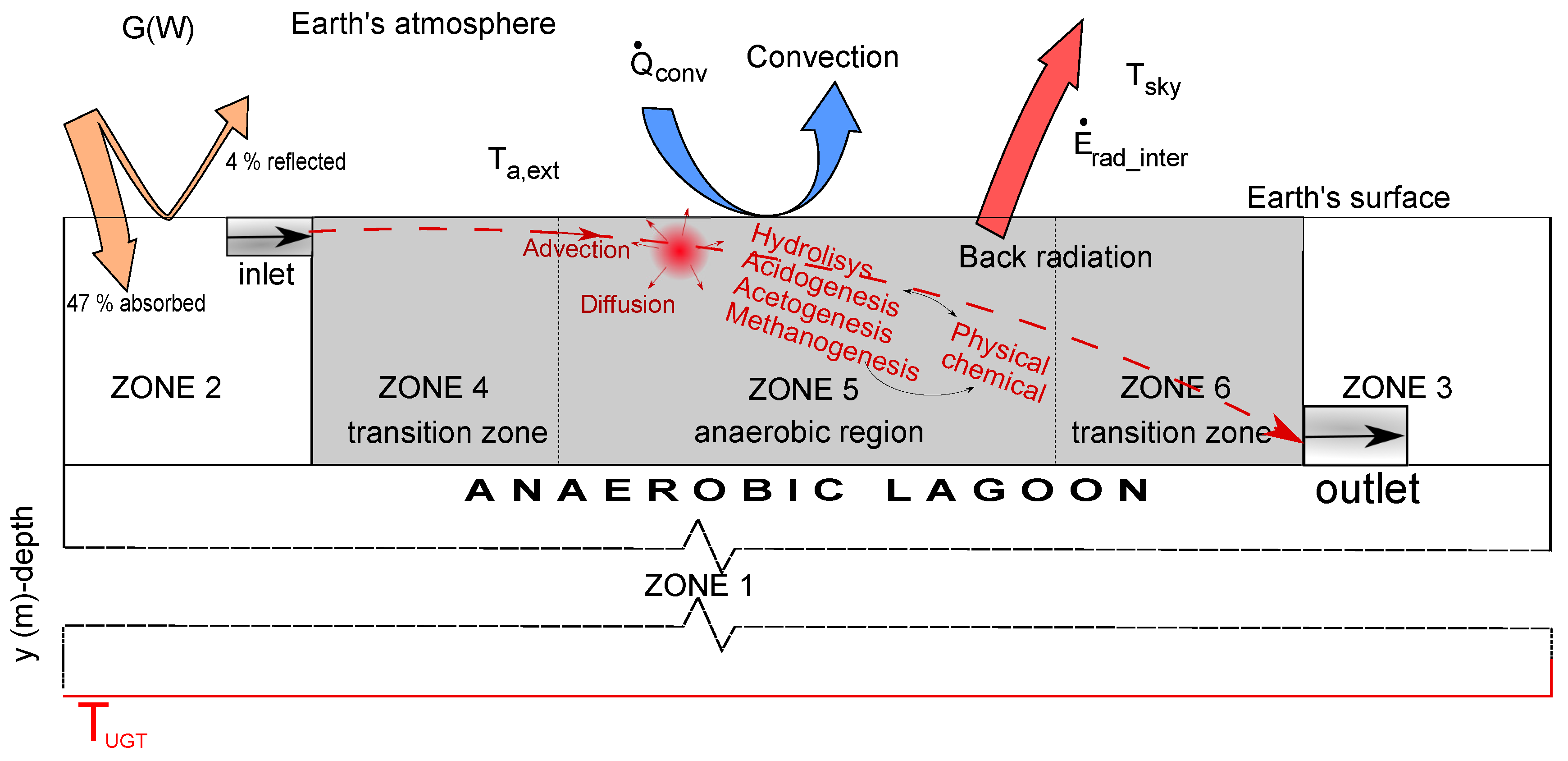
2.1. Overview

Pollutant is removed in AL through combination of physical, biochemical and physical–chemical phenomena. Advection, diffusion and heat transfer are the most common physical processes in these systems (Figure 1). Both the organic matter and the suspended microorganism within lagoons are subjected to the mechanical transport with the bulk flow of the water (advection). At the same time, they tend to spread out and diffuse from higher to lower concentration as time varies (diffusion). The energy transfer in the system, due to a temperature gradient (heat transfer), is performed by conduction and convection processes. Atmospheric factors associated with the borders of the model on the Earth‘s surface include, beside the two previous, radiation process. Digestion process is carried by anaerobic microorganism’s activity, bacteria an archaea, through a number of sequential and parallel reactions. The biochemical reactions consist of irreversible five-stage processes; disintegration, hydrolysis, acidogenesis, acetogenesis and methanogenesis reactions. Physical–chemical reactions are those reversible processes where cells are not involved. They are, firstly, the ion association/dissociation, and gas–liquid transfer [14].

Considering a system where the lagoon and its environment are included, different zones can be identified (Figure 1). Depending on the local parameters—thermal conductivity, specific heat, density, and where biological processes take place—they are considered different zones. Boundary conditions are located on the borders. Undisturbed ground temperature $T_{UGT}$ is a ground thermal property situated at a depth where the ground temperature is approximately invariable, depth value depends on climatic conditions and is different in various regions of the Earth [23,24].

2.2. Governing Equations (Strong Formulations)

In this research, the mathematical model proposed is based on the two-dimensional advection–diffusion-reaction, Stokes, and heat transfer equations. This is accompanied by a series of boundary conditions. On the other hand, the IWA Anaerobic Digestion Model 1 (ADM1) has been implemented in the model.

The description of the model has been expressed in terms of primitive variables, mass, velocity, pressure, and temperature. In these equations it has been assumed that velocity and temperature field are in steady state conditions.

2.2.1. Advection–Diffusion Reaction Equation

Advection–diffusion-reaction Equation (ADRE) as numerical solution, widely used within mathematical modelling, to describe physical, biochemical and physical–chemical processes in AL [19,25,26,27].

Governing equations and boundary conditions are summarized below.

$$\begin{array}{cc}\hfill \frac{\partial \varphi }{\partial t}-\mathfrak{D}\Delta \varphi +\overrightarrow{u}\nabla \varphi +f\left(\varphi \right)=F(x,y)& forx,yϵ\mathsf{\Omega }\hfill \\ \hfill \varphi (x,y,t)=g_D(x,y)& forx,yϵ{\mathsf{\Gamma }}_D\subset \partial \mathsf{\Omega },t>0\hfill \\ \hfill \frac{\partial \varphi (x,y,t)}{\partial n}n(x,y)=g_N(x,y)& forx,yϵ{\mathsf{\Gamma }}_N\subset \partial \mathsf{\Omega },t>0\hfill \end{array}$$

(1)

where ($\varphi$) is a scalar field that represent concentrations of both substrates and cells of each of the biochemical reactions included in the anaerobic processes, $\overrightarrow{u}=(u_1,u_2)$ is given by Equations (2), $f\left(\varphi \right)$ is the source function, which is positive $f\left(\varphi \right)>0$ for growth and production or negative $f\left(\varphi \right)<0$ for decay and consumption, biomass and metabolites, respectively, ${\mathsf{\Gamma }}_D$ and ${\mathsf{\Gamma }}_N$ are Dirichlet and Neumann boundary conditions, respectively. This term is developed in Equation (7), $F(x,y)$ is a generation function, which is zero $\left(0\right)$ in this case.

2.2.2. Stokes Equation

Stokes equation, together with the ADR has been used to describe the flow. It is usually used for fluid with slowly motion and with high viscosity [28,29]. In this research, a constant density and incompressible Newtonian fluid flow has been considered. Strong formulation and Dirichlet ${\mathsf{\Gamma }}_D$ and ${\mathsf{\Gamma }}_N$ boundary conditions are as follow.

$$\begin{array}{cc}\hfill -\nu \Delta \overrightarrow{u}+\nabla p=\overrightarrow{F}& forx,yϵ\mathsf{\Omega }\hfill \\ \hfill \nabla \overrightarrow{u}=0& forx,yϵ\mathsf{\Omega }\hfill \\ \hfill \overrightarrow{u}=\overrightarrow{u_0}& forx,yϵ{\mathsf{\Gamma }}_D\hfill \\ \hfill \nabla \overrightarrow{u}·n+pn=g& forx,yϵ{\mathsf{\Gamma }}_N\hfill \end{array}$$

(2)

2.2.3. The Energy Equation—Temperature Distribution

The energy equation is based on the conservation of energy and the Fourier heat conduction laws [30]. The internal energy balance equations, under a steady-state Eulerian description can be expressed as a function of temperature [30,31]

$$\begin{array}{cc}\hfill {\rho }_0{C}_v(\overrightarrow{u}\nabla T)-\nabla (k_i\nabla T)=0& forx,yϵ\mathsf{\Omega }\hfill \\ \hfill T(x,y)=T_{aa}(x,y)& forx,yϵ{\mathsf{\Gamma }}_D\hfill \\ \hfill \frac{\partial T(x_i,t)}{\partial n}n\left(x_i\right)=g_N\left(x_i\right)& forx,yϵ{\mathsf{\Gamma }}_N\hfill \\ \hfill k{\displaystyle \frac{\partial T}{\partial n}}=h(T_{a,ext}-T)+{\epsilon }_s·\sigma ·(T^4-T_{sky}^4)& forx,yϵ{\mathsf{\Gamma }}_R\hfill \end{array}$$

(3)

where ${\mathsf{\Gamma }}_D$ corresponds to Dirichlet condition. It is applied to the UGT (Figure 1); ${\mathsf{\Gamma }}_N$ is the Neumann condition. It describes the value of the gradient of the dependent field variable, normal to the boundary. Its calculation is based on Fourier Law; ${\mathsf{\Gamma }}_R$ is the Robin condition. It describes the Earth’s surface heating and cooling ${\mathsf{\Gamma }}_R$. This implied the use of Stefan–Boltzmann’s law and Newtons’ law of cooling to model the heat exchange, related to radiation and convection processes, respectively [32,33]. Stefan–Boltzmann constant is $\sigma =5.68·{10}^{-8}(\mathrm{W}·{\mathrm{K}}^{-4}·{\mathrm{m}}^{-2})$ [34]; $T_{a,ext}$ temperature of the externally surrounding surface; ${\epsilon }_s$ is the Earths’ surface emissivity, where $0\le {\epsilon }_s\le 1$; $T_{sky}$ is the sky radioactive temperature. These are used to estimate the radiative heat exchange with the Earth’s atmosphere [35]. $T_{sky}$ and ${\epsilon }_{sky}$ is used to estimate the radiative heat exchange with the Earth’s atmosphere [35].

$$T_{sky}={\left(\frac{{\epsilon }_{sky}·T_{a,ext}^4}{\sigma }\right)}^{\frac{1}{4}}-273.15$$

(4)

$${\epsilon }_{sky}=\left(0.787+0.764ln\left(\frac{T_{dp}}{273}\right)\right)(1+0.0224N+0.0035N^2+2.8·{10}^{-4}{N}^3)$$

(5)

such $0\le {\epsilon }_{sky}\le 1$.

Here N are tenths cloud cover, and $T_{dp}\left(K\right)$ is the dew-point temperature to which it must be cooled to become saturated. It is obtained by a correlation found in [33] (6) and

$$T_{dp}=T-\left(\frac{100-RH}{5}\right)$$

(6)

In this work, heat sources from biochemical reactions have not been considered.

2.2.4. Kinetic Equations

ADM1 is used for the description $f\left(\varphi \right)$ (Equation (1)). Biochemical rate coefficients and kinetic rate equations are represented in the Tables S1 and S2 within the Supplementary Materials Section. First order kinetic was considered for the hydrolysis, acidogenesis, acetogenesis and methanogenesis. The following equations based on common kinetic expressions describe anaerobic treatment processes:

$$f\left(S_i\right)=-\frac{\partial S_i}{\partial t}=-{\rho }_j\frac{Xi}{Yi};f\left(X_i\right)=\frac{\partial X_i}{\partial t}={\rho }_j{X}_i-K_{d}Xi;{\rho }_j={\mu }_{ma{x}_i}{\displaystyle \frac{S_i}{K_{s_1}+S_i}}·I_1·I_2···I_n$$

(7)

$f\left(S_i\right)$ and $f\left(X_i\right)$ are the changes in substrates and cells concentration over time. These equations are based on the monod-type reaction kinetics [13,36]. In this model, it has been considered free ammonia and pH inhibitions, in addition to the butyrate and valerate competition [19].

The influence of temperature has been obtained by the Cardinal Temperature Model 1 (Appendix A) proposed by [37]

$${\mu }_{max}={\mu }_{opt}\frac{(T-T_{max}){(T-T_{min})}^2}{(T_{opt}-T_{min})[(T_{opt}-T_{min})(T-T_{opt})-(T_{opt}-T_{max})(T_{opt}+T_{min}-2T)]}$$

(8)

2.3. Solution Procedure

The finite element method, numerical technique based on the generation of a finite element geometric model, is used for the solution of the partial differential equations including in the problem.

In this methodology, the major steps include

• The approach of the weak forms from the governing equations. The solutions are assumed to belong to Hilbert space, considering this space as an infinite dimensional function space with functions of specific properties that can be suitably managed in the same way as ordinary vectors in a vector space. They are represented in

  Table 1. Scheme of the weak equations used in the model, where $\overrightarrow{v},q,Y_i,W$ are the smooth functions and ${\mathbb{H}}_0^1,{\mathbb{P}}_0^1,{\mathbb{P}}_0^2$ are the Hilbert space.

  Model	Weak Equations	Hilbert Spaces
  Stokes	$\mu {\int }_{\mathsf{\Omega }}\nabla \overrightarrow{u}·\nabla \overrightarrow{v}-{\int }_{\mathsf{\Omega }}\left(div\overrightarrow{v}\right)p={\int }_{\mathsf{\Omega }}\overrightarrow{f}\overrightarrow{v}$	$forall\overrightarrow{v}ϵ{\mathbb{P}}_0^2\left({\tau }^h\right)$
  	${\int }_{\mathsf{\Omega }}\left(div\overrightarrow{u}\right)q=0$	$forallqϵ{\mathbb{P}}_0^1\left({\tau }^h\right)$
  ADR	${\int }_{\mathsf{\Omega }}\frac{\partial \varphi }{\partial t}·Y_i+\mathfrak{D}{\int }_{\mathsf{\Omega }}\nabla \varphi ·\nabla Y_i+{\int }_{\mathsf{\Omega }}u\nabla \varphi ·Y_i+{\int }_{\mathsf{\Omega }}f\left(\varphi \right)·Y_i=F\left(x_i\right)·Y_i$	$forall{Y}_iϵ{\mathbb{H}}_0^1\left(\mathsf{\Omega }\right)$
  Thermal	${\int }_{\mathsf{\Omega }}W$$\left[-\frac{\partial }{\partial x,y}(k\frac{\partial T}{\partial x,y}-\frac{\partial }{\partial xj}\left(k\frac{\partial T}{\partial xj}\right)-q_c(x,y,xj)\right]dxi$	$forallTϵ{\mathbb{P}}_0^2\left({\tau }^h\right)$

  .
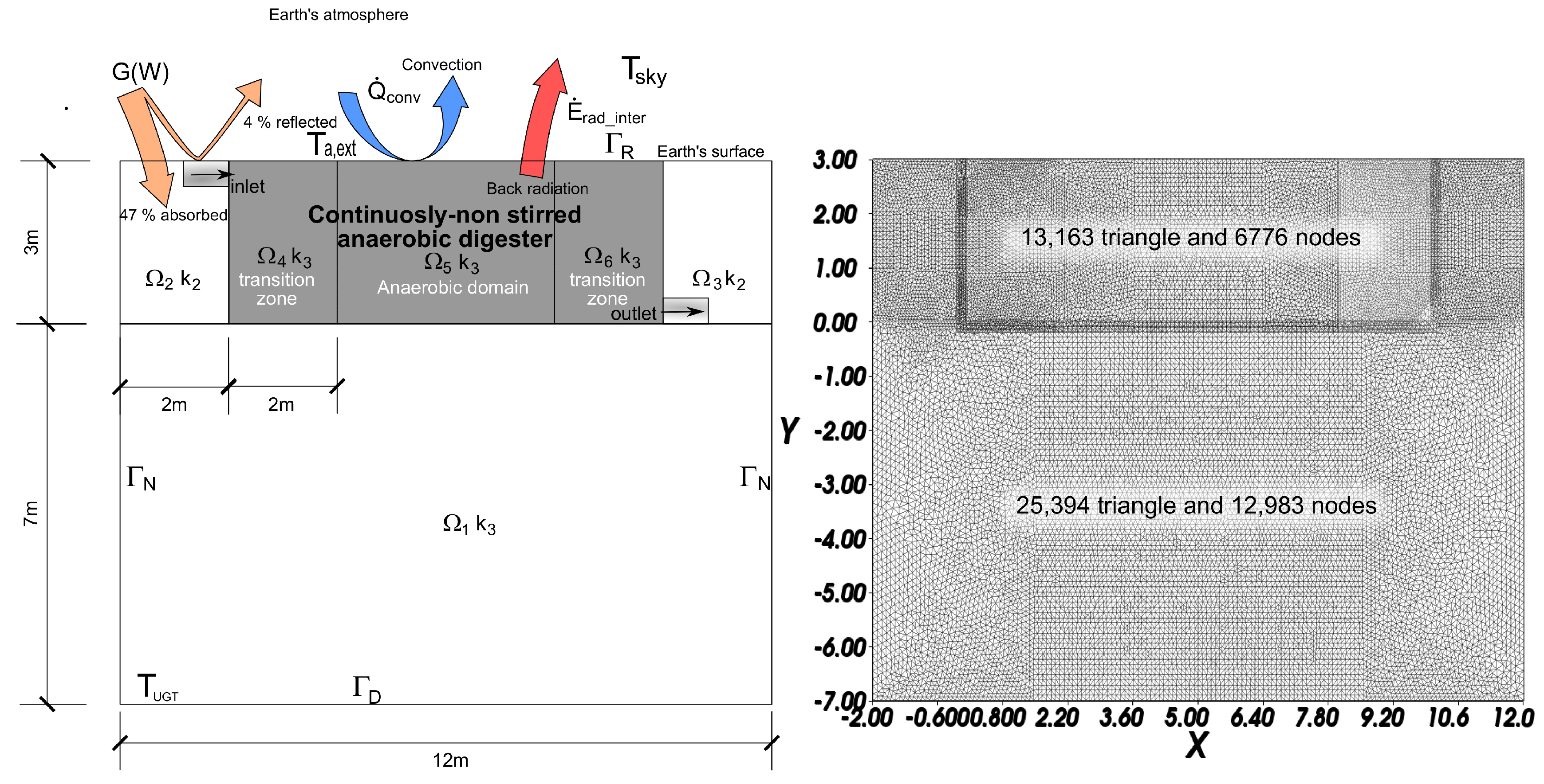
• Discretization of the domains, both physical with more or less regular triangulation and related to time. In Figure 2, the discretization of the different sub-domains, nodes and triangle, is showed.
• Selection of the shape functions, essential to provide an approximation of the solution within an element. These relate the coordinates of every point of a finite element with the positions of its nodes,
• Formulation of the system of equations.
• Solving systems of equations. The free software FreeFem++ has been used to solve them. It is a PDE solver with its own high-level programming language and accurate syntax for mathematical formulation. Freefem++ have high diversity of triangular finite elements (linear and quadratic, Lagrangian elements, discontinuous $P^2$, etc.) to solve PDE in two (2D) and three (3D) dimensions.

2.4. Calculation

The partial differential equation solver FreeFem++ was used to implement the algorithm for the calculation. Due to it advantages, open access software with a powerful generated mesh and a large collection package to visualize approximate solutions, makes Freefem++ an ideal tool to solve complex partial differential equations [38]. Parallel calculation by parallel computing on clusters of personal computer has been achievable with a Message Passing Interface (MPI) within Freefem++.

3. Results and Discussion

3.1. Model’s Considerations

In order to solve the formulated problem, fitted for a specific case, it has been necessary to stablish geometric conditions, physical properties, initial conditions and boundary values. A summary of these characteristics is represented in Figure 2,

Table 2. General parameters considered. Q represents hydraulic flow in the inlet and outlet pipe. $S_i$ and $X_i$ represent substrate and cell concentrations in the inlet pipe.

Thermal Constants						Diffusion Coefficient	Boundary Values
$cos\mathsf{\Theta }$	$h_{int}$	$\sigma$	$k_1$	$k_2$	$k_3$	$\mathfrak{D}$	Q	$S_i$	$X_i$
($\mathrm{W}·{\mathrm{m}}^{-2}$)	($\mathrm{W}·{\mathrm{m}}^{-2}·{\mathrm{K}}^{-1}$)	($\mathrm{W}·{\mathrm{m}}^{-2}·{\mathrm{K}}^{-4}$)	(${\mathrm{m}}^2·{\mathrm{d}}^{-1}$)			${\mathrm{m}}^2·{\mathrm{d}}^{-1}$	(${\mathrm{m}}^3·{\mathrm{d}}^{-1}$)	($\mathrm{mg}(\mathrm{COD})·{\mathrm{L}}^{-1}$)
0.29	10	$5.67·{10}^{-8}$	2.3	3	0.02	$8.64·{10}^{-3}$	0.5	28,000	110–150

,

Table 3. Kinetic parameters [6].

Kinetic Parameters	Sugar	Fats	Amino Acids	Propionate	Butyrate	LFCA	Valerate	Acetic Acid
${\mu }_{opt}\left({\mathrm{d}}^{-1}\right)$	6.9	3.9	6.9	0.49	0.67	6.1	1.1	7.5
$K_d\left({\mathrm{d}}^{-1}\right)$	0.9	1	1	0.04	0.03	0.25	0.04	0.037
$K_s\left(\mathrm{kg}{\left(\mathrm{COD}\right)/\mathrm{m}}^3\right)$	0.5	0.8	3	1.145	0.176	0.8	0.5	0.037

and

Table 4. Specific weather parameters considered from four wastewater treatment plants (WWTP). It is provided the Universal Transverse Mercator (UTM) coordinates. $T_{am}$ are the annual means temperatures and $T_{mm}$ the monthly means. P1 and P3 are located in the coastal zones, while P2 and P4 are located in the mid-altitude zones.

WWTP	UTM Coordinate			wind ($\mathbf{m}·{\mathbf{s}}^{-1}$)	${\mathit{T}}_{\mathit{am}}$${}^{\circ }$C	${\mathit{T}}_{\mathit{mm}}$	RH (%)	G	${\mathit{T}}_{\mathit{dp}}$	$\mathit{\epsilon }$	${\mathit{T}}_{\mathit{sky}}$
	x	y	z					(${\mathbf{W}/\mathbf{m}}^2$)	(${}^{\circ }$C)		(${}^{\circ }$C)
P1	430,371	3,108,919	11.60	6.6	22.7	19.0	64	290.53	11.8	0.822	5.00
P2	444,484	3,108,895	511	6.6	19.8	16.6	82	278.80	13.0	0.824	2.95
P3	428,778	3,084,390	271.81	5.3	22.2	19.3	66	299.39	12.5	0.823	5.41
P4	447,661	3,098,525	831.51	5.3	17.3	12.9	80	292.68	8.9	0.813	−1.53

and in the Supplementary Materials Section.

The system has been divided in different domains and subdomains. ${\mathsf{\Omega }}_1$, ${\mathsf{\Omega }}_2$ and ${\mathsf{\Omega }}_3$ are included within ${\mathsf{\Omega }}_g$ and refer to the immediate ground around of lagoon; whereas ${\mathsf{\Omega }}_4$, ${\mathsf{\Omega }}_5$ and ${\mathsf{\Omega }}_6$ in ${\mathsf{\Omega }}_r$ and concern the lagoon. AD occurs in ${\mathsf{\Omega }}_5$ considering ${\mathsf{\Omega }}_4$ and ${\mathsf{\Omega }}_6$ as transition zones (Figure 2).

In this case, the proposed anaerobic lagoon is located in temperate zones and is subjected to the environmental thermal conditions considering that there are no thermal loads on the sides of the domains, so the ground heat flow is transmitted vertically.

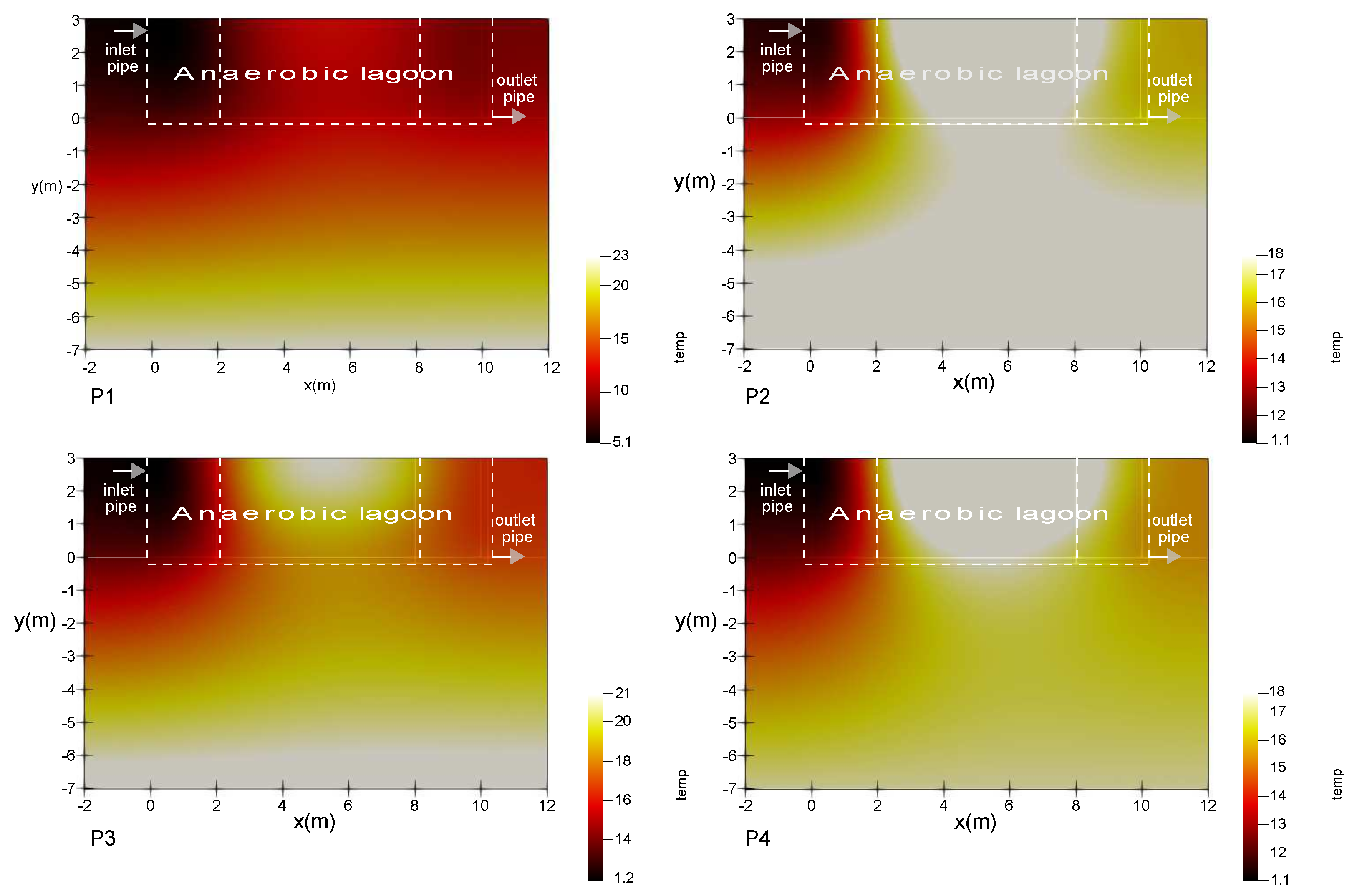
3.2. Evaluation on Performance of Temperature

Figure 3 shows the temperature distribution in the proposed system under steady-state conditions for some examples of wastewater treatment plants whose information is included in Table 4. The lagoon contour has been illustrated in the first graphic. It is of interest to observe how the thermal behaviour within the lagoon depends on the boundary conditions, but also the hydraulic flow that is subject to the boundary values in the inlet and outlet pipe.

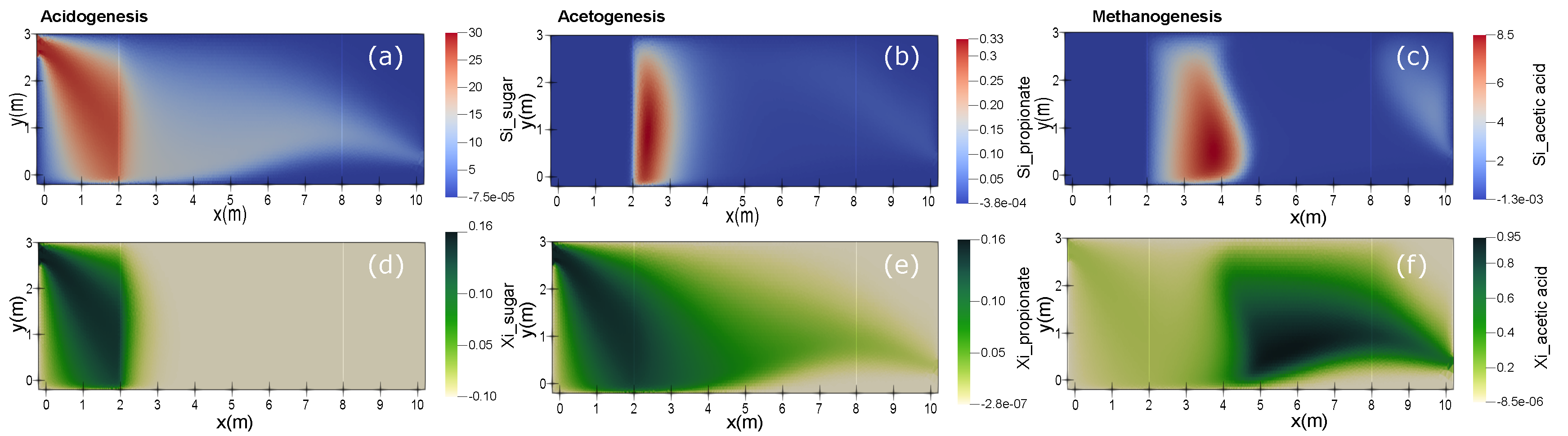
3.3. Organic Matter Removal and Behaviour of the Microbial Community

Figure 4 represents the variation on concentrations, in steady state, happening in some of the processes taking place within the lagoon. These simulations describe, in the case of P1 (Table 4), the variation of sugar, propionate, acetic acid and their corresponding bacterial biomass concentration, along of the pond’s length and depth, according to the boundary conditions as shown in Table 2.

As shown in these simulations, concentrations decreased throughout the pond length as a result of dispersion and biodegradation. The transition zones (Figure 2) have been considered as low microbial activity, so the net growth of cells is observable from the x-axis value equal to 2. As a result, propionate and acetic acid’s source are located in this zone (${\mathsf{\Omega }}_5$). The cells’ growth is affected much more by the concentration of the substrates than the temperature’s effects because temperature variations in this region differ very little from one point to another.

With respect to acidogenesis and methanogenesis, cells effectiveness on substrates removal is greater than in the acetogenesis due to the kinetic parameters. For the propionate ${\mu }_{max}$ and $K_s$ are $0.49\left({\mathrm{d}}^{-1}\right)$ and $1.145(\mathrm{mg}\left(\mathrm{COD}\right)·{\mathrm{m}}^{-3})$, respectively, (see Table 3). Thus, cells growth value and, therefore, the substrate removal is lower than in the previous two cases (see Equation (7)). The resulting value of substrate concentration in the outlet, after the wastewater treatment process, is between 600 and 500 (mg(COD)/L). In the case of acetic acid, this same concentration, next to the pond outlet, is smaller, due to the accumulation of organic matter that has not been reached by the microbial community.

Figure 5 shows charts representing substrate and propionic acid bacteria’s concentrations for P1 (Table 4) along the axis AA. Cases 1 and 2, with different concentrations of microorganisms in the inlet pipe of the lagoon, 110 (mg(COD)$·{\mathrm{L}}^{-1})$ and 115 (mg(COD)$·{\mathrm{L}}^{-1})$, respectively, are compared. In both cases, the graphics share a similar trend, a downward slope which, al last, connects at the middle point of the axis. There is no net growth within the microbial population. The slope above mentioned is reduced, cells growth offsets the diffusion process in ${\mathsf{\Omega }}_5$ (Figure 2). Nevertheless, substrate removal in Case 2 is benefited by the highest concentration of cells at the inlet pipe 150 (mg(COD)$·{\mathrm{L}}^{-1})$. The decrease in values from the last section, for both graphs, occurs as a result of the dispersion phenomenon since microbial activity in ${\mathsf{\Omega }}_6$ has not been considered.

Figure 6 depicts, as in the previous example, the chart of propionate along the axis AA as well as the distribution of temperature in the lagoon for three different examples. E-1; The lagoon is subjected to ambient temperature (see case P4 in Table 4 and Figure 3). E-2; It is included a bed heat source at the bottom of the lagoon, between 2 and 3 coordinates of the x axis with a temperature of 35 ${}^{\circ }$C. E-3; In this occasion, that same heat source is located between coordinates 4 and 8 of the x axis.

The distribution of temperature is showed in Figure 3 and Figure 6. As expected, the removal efficiency is improved by the rising temperature of the heat source, as is observed in the cases 2 and 3. However, this graphic also shows that organic matter is eliminated more efficiently in case 2 than in 3 in a percentage of 10 %. Consequently a minor residual concentration in the outlet pipe is achieved.

Table 5. Values of propionate concentrations and the rate per 100 removed.

Case	Source	Effluent	Removed	Percentage
	Si (mg(COD)/L)	Si (mg(COD)/L)	(mg(COD)/L)	Removed
1	1500	280	1220	81.33%
2	1500	265	1235	82.33%
3	1700	215	1485	87.35%
4	1400	135	1265	90.35%

sums up the propionate removal information for the four examples above mentioned. It shows the source and effluent concentrations, as well as the percentage removed. Best values correspond with case 4.

By analysing the table, it can be said that the propionate concentration at the outlet of the lagoon, once acetogenic bacteria have removed a great part of substrate in the system, is among 280 and 135 mg$·{\mathrm{L}}^{-1}$. By placing a heat source, strategically, at the bottom of the lagoon (E-2 and E-3) it is possible to reduce substrate concentrations at its outlet.

4. Conclusions

In this paper, we have proposed and assessed a methodology for anaerobic cells performance for wastewater treatment, in AL, under the influence of the temperature. It has been studied in terms of biomass and substrate concentrations. The model couples a series of PDEs, related to the phenomena associated to AL (ADRE, ADM1, Stokes and heat transfer), to each other.

Diffusion for horizontal and vertical directions, the movement of the bulk of the concentrations in accordance with a gradient, external temperature interactions, biochemical and physical–chemical reactions, and a set of boundary values were considered in this study.

This model builds understanding for microbial community’s behaviour along the lagoon as a function of the temperature. Applying heat load in different points of the system, it has been possible to establish correlations through the graphics, as well as the comparison between diverse scenarios according to their corresponding boundary values. The results give us the possibility to obtain effective designs adapted to each circumstance, avoiding energy loss.

This methodology allows the optimization of unstirred flow systems, taking into account that the advantages of these systems make them more suitable for specific applications. The model can be used in the prediction of the effluent quality and in the design of AL to achieve better performances.

In view of the results, it can be concluded that this methodology has significant potential as a tool for both the design of AL, and the interactive learning of the microbial ecology in plug flow systems.

References

1. Parralejo, A.; Royano, L.; González, J.; González, J. Small scale biogas production with animal excrement and agricultural residues. Ind. Crops Prod. 2019, 131, 307–314. [Google Scholar] [CrossRef]
2. Holm-Nielsen, J.; Seadi, T.A.; Oleskowicz-Popiel, P. The future of anaerobic digestion and biogas utilization. Bioresour. Technol. 2009, 100, 5478–5484. [Google Scholar] [CrossRef]
3. Park, J.H.; Park, J.H.; Lee, S.H.; Jung, S.P.; Kim, S.H. Enhancing anaerobic digestion for rural wastewater treatment with granular activated carbon (GAC) supplementation. Bioresour. Technol. 2020, 315, 123890. [Google Scholar] [CrossRef] [PubMed]
4. Jiang, Y.; Bebee, B.; Mendoza, A.; Robinson, A.K.; Zhang, X.; Rosso, D. Energy footprint and carbon emission reduction using off-the-grid solar-powered mixing for lagoon treatment. J. Environ. Manag. 2018, 205, 125–133. [Google Scholar] [CrossRef] [PubMed]
5. Duan, N.; Zhang, D.; Khoshnevisan, B.; Kougias, P.G.; Treu, L.; Liu, Z.; Lin, C.; Liu, H.; Zhang, Y.; Angelidaki, I. Human waste anaerobic digestion as a promising low-carbon strategy: Operating performance, microbial dynamics and environmental footprint. J. Clean. Prod. 2020, 256, 120414. [Google Scholar] [CrossRef]
6. Mendieta-Pino, C.A.; Ramos-Martin, A.; Perez-Baez, S.O.; Brito-Espino, S. Management of slurry in Gran Canaria Island with full-scale natural treatment systems for wastewater (NTSW). One year experience in livestock farms. J. Environ. Manag. 2019, 232, 666–678. [Google Scholar] [CrossRef]
7. Muga, H.; Mihelcic, J. Sustainability of wastewater treatment technologies. J. Environ. Manag. 2008, 88, 437–447. [Google Scholar] [CrossRef]
8. Wu, B.; Chen, Z. An integrated physical and biological model for anaerobic lagoons. Bioresour. Technol. 2011, 102, 5032–5038. [Google Scholar] [CrossRef]
9. Wu, B. Advances in the use of CFD to characterize, design and optimize bioenergy systems. Comput. Electron. Agric. 2013, 93, 195–208. [Google Scholar] [CrossRef]
10. Donoso-Bravo, A.; Sadino-Riquelme, C.; Gómez, D.; Segura, C.; Valdebenito, E.; Hansen, F. Modelling of an anaerobic plug-flow reactor. Process analysis and evaluation approaches with non-ideal mixing considerations. Bioresour. Technol. 2018, 260, 95–104. [Google Scholar] [CrossRef]
11. Rajeshwari, K.; Balakrishnan, M.; Kansal, A.; Lata, K.; Kishore, V. State-of-the-art of anaerobic digestion technology for industrial wastewater treatment. Renew. Sustain. Energy Rev. 2000, 4, 135–156. [Google Scholar] [CrossRef]
12. Lauwers, J.; Appels, L.; Thompson, I.P.; Degrève, J.; Impe, J.F.V.; Dewil, R. Mathematical modelling of anaerobic digestion of biomass and waste: Power and limitations. Prog. Energy Combust. 2013, 39, 383–402. [Google Scholar] [CrossRef]
13. Wade, M.; Harmand, J.; Benyahia, B.; Bouchez, T.; Chaillou, S.; Cloez, B. Perspectives in mathematical modelling for microbial ecology. Ecol. Model. 2016, 321, 64–74. [Google Scholar] [CrossRef]
14. Batstone, D.; Keller, J.; Angelidaki, I.; Kalyuzhnyi, S.; Pavlostathis, S.; Rozzi, A.; Sanders, W.; Siegrist, H.; Vavilin, V. The IWA Anaerobic Digestion Model No 1 (ADM1). Water Sci. Technol. 2002, 45, 65–73. Available online: http://xxx.lanl.gov/abs/http://wst.iwaponline.com/content/45/10/65.full.pdf (accessed on 1 September 2020). [CrossRef] [PubMed]
15. Kleerebezem, R.; van Loosdrecht, M.C.M. Critical analysis of some concepts proposed in ADM1. Water Sci. Technol. 2006, 54, 51–57. [Google Scholar] [CrossRef]
16. Li, D.; Lee, I.; Kim, H. Application of the linearized ADM1 (LADM) to lab-scale anaerobic digestion system. J. Environ. Chem. Eng. 2021, 9, 105193. [Google Scholar] [CrossRef]
17. Fleming, J.G. Novel Simulation of Anaerobic Digestion Using Computational Fluid Dynamics. Ph.D. Thesis, North Carolina State University, Raleigh, NC, USA, 2002. [Google Scholar]
18. Goodarzi, D.; Sookhak Lari, K.; Mossaiby, F. Thermal effects on the hydraulic performance of sedimentation ponds. J. Water Process. Eng. 2020, 33, 101100. [Google Scholar] [CrossRef]
19. Brito-Espino, S.; Ramos-Martín, A.; Pérez-Báez, S.; Mendieta-Pino, C. Application of a mathematical model to predict simultaneous reactions in anaerobic plug-flow reactors as a primary treatment for constructed wetlands. Sci. Total Environ. 2020, 713, 136244. [Google Scholar] [CrossRef] [PubMed]
20. Mahmudul, H.; Rasul, M.; Akbar, D.; Narayanan, R.; Mofijur, M. A comprehensive review of the recent development and challenges of a solar-assisted biodigester system. Sci. Total Environ. 2021, 753, 141920. [Google Scholar] [CrossRef]
21. Atelge, M.; Atabani, A.; Banu, J.R.; Krisa, D.; Kaya, M.; Eskicioglu, C.; Kumar, G.; Lee, C.; Yildiz, Y.; Unalan, S.; et al. A critical review of pretreatment technologies to enhance anaerobic digestion and energy recovery. Fuel 2020, 270, 117494. [Google Scholar] [CrossRef]
22. Tumilar, A.S.; Milani, D.; Cohn, Z.; Florin, N.; Abbas, A. A Modelling Framework for the Conceptual Design of Low-Emission Eco-Industrial Parks in the Circular Economy: A Case for Algae-Centered Business Consortia. Water 2021, 13, 69. [Google Scholar] [CrossRef]
23. Haßler, S.; Ranno, A.M.; Behr, M. Finite-element formulation for advection–reaction equations with change of variable and discontinuity capturing. Comput. Methods Appl. Mech. Eng. 2020, 369, 113171. [Google Scholar] [CrossRef]
24. Mirza, I.A.; Akram, M.S.; Shah, N.A.; Imtiaz, W.; Chung, J.D. Analytical solutions to the advection-diffusion equation with Atangana-Baleanu time-fractional derivative and a concentrated loading. Alex. Eng. J. 2021, 60, 1199–1208. [Google Scholar] [CrossRef]
25. Singh, S.; Bansal, D.; Kaur, G.; Sircar, S. Implicit-explicit-compact methods for advection diffusion reaction equations. Comput. Fluids 2020, 212, 104709. [Google Scholar] [CrossRef]
26. Zeng, L.; Chen, G. Ecological degradation and hydraulic dispersion of contaminant in wetland. Ecol. Model. 2011, 222, 293–300. [Google Scholar] [CrossRef]
27. Bozkurt, S.; Moreno, L.; Neretnieks, I. Long-term processes in waste deposits. Sci. Total Environ. 2000, 250, 101–121. [Google Scholar] [CrossRef]
28. Song, L.; Li, P.W.; Gu, Y.; Fan, C.M. Generalized finite difference method for solving stationary 2D and 3D Stokes equations with a mixed boundary condition. Comput. Math. Appl. 2020, 80, 1726–1743. [Google Scholar] [CrossRef]
29. Ukai, S. A solution formula for the Stokes equation in Rn+. Commun. Pure Appl. Math. 1987, 40, 611–621. [Google Scholar] [CrossRef]
30. Reddy, J.; Gartling, D. The Finite Element Method in Heat Transfer and Fluid Dynamics, 3rd ed.; CRC Press: Boca Raton, FL, USA, 2010; pp. 1–483. [Google Scholar]
31. Alvarez-Hostos, J.C.; Bencomo, A.D.; Puchi-Cabrera, E.S.; Fachinotti, V.D.; Tourn, B.; Salazar-Bove, J.C. Implementation of a standard stream-upwind stabilization scheme in the element-free Galerkin based solution of advection-dominated heat transfer problems during solidification in direct chill casting processes. Eng. Anal. Bound. Elem. 2019, 106, 170–181. [Google Scholar] [CrossRef]
32. Guldentops, G.; Van Dessel, S. A numerical and experimental study of a cellular passive solar façade system for building thermal control. Sol. Energy 2017, 149, 102–113. [Google Scholar] [CrossRef]
33. Lawrence, M.G. The Relationship between Relative Humidity and the Dewpoint Temperature in Moist Air: A Simple Conversion and Applications. Bull. Am. Meteorol. Soc. 2005, 86, 225–234. [Google Scholar] [CrossRef]
34. Çengel, Y. Heat Transfer: A Practical Approach. In McGraw-Hill Series in Mechanical Engineering; McGraw Hill Books: London, UK, 2003. [Google Scholar]
35. Walton, G.N. Thermal Analysis Research Program Reference Manual; NBSIR, Department of Energy, Office of Building Energy Research and Development: Washington, DC, USA, 1983. [Google Scholar]
36. Monod, J. The Growth of Bacterial Cultures. Annu. Rev. Microbiol. 1949, 3, 371–394. [Google Scholar] [CrossRef]
37. Rosso, L.; Lobry, J.; Flandrois, J. An Unexpected Correlation between Cardinal Temperatures of Microbial Growth Highlighted by a New Model. J. Theor. Biol. 1993, 162, 447–463. [Google Scholar] [CrossRef]
38. Herus, V.A.; Ivanchuk, N.V.; Martyniuk, P.M. A System Approach to Mathematical and Computer Modeling of Geomigration Processes Using Freefem++ and Parallelization of Computations. Cybern Syst. Anal. 2018, 54, 284–292. [Google Scholar] [CrossRef]
39. Donoso-Bravo, A.; Bandara, W.; Satoh, H.; Ruiz-Filippi, G. Explicit temperature-based model for anaerobic digestion: Application in domestic wastewater treatment in a UASB reactor. Bioresour. Technol. 2013, 133, 437–442. [Google Scholar] [CrossRef] [PubMed]
40. Donoso-Bravo, A.; Retamal, C.; Carballa, M.; Ruiz-Filippi, G.; Chamy, R. Influence of temperature on the hydrolysis, acidogenesis and methanogenesis in mesophilic anaerobic digestion: Parameter identification and modeling application. Water Sci. Technol. 2009, 60, 9–17. [Google Scholar] [CrossRef] [PubMed]
Figure 1. Scheme of the different phenomena that take places in AL and their environments.
Water 13 00882 g001
Figure 2. (left) geometric characteristics and boundary values; (right) dicretization of the domains.
Water 13 00882 g002
Figure 3. Temperature distribution under four different scenarios, according to the characteristic parameter exposed in Table 4.
Water 13 00882 g003
Figure 4. Concentrations’ variation, together with the length and depth of the lagoon, for the example P1. (ac) correspond to substrates, (df) to microorganisms.
Water 13 00882 g004
Figure 5. Performance of propionate, in steady state, for two different cases according to the initial concentration of propionic acetogenic bacteria and their graphic presentations along the axis AA. Case1; 110 ( mg ( COD ) · L 1 ) , Case2; 115 ( mg ( COD ) · L 1 ) .
Water 13 00882 g005
Figure 6. (a) Temperature distribution under three different scenarios; E-1 Ambient temperature, E-2 includes a heat source at the bottom of the lagoon, between coordinates 2 and 4, and the E-3 between 4 and 8, in the x axis. (b,c) Concentration of propionate and cells, respectively, along the axis AA (see Figure 5) for the different scenarios detailed in (a).
Water 13 00882 g006