
Developing Pseudo Continuous Pedotransfer Functions for International Soils Measured with the Evaporation Method and the HYPROP System: II. The Soil Hydraulic Conductivity Curve


Abstract
1. Introduction
2. Materials and Methods
2.1. Soil Data Sets
2.2. Unsaturated Hydraulic Conductivity Calculations
2.3. PCNN-PTFs Development
2.4. Modeling Scenarios
2.5. Model Evaluation
3. Results
3.1. Importance of the Input Predictors
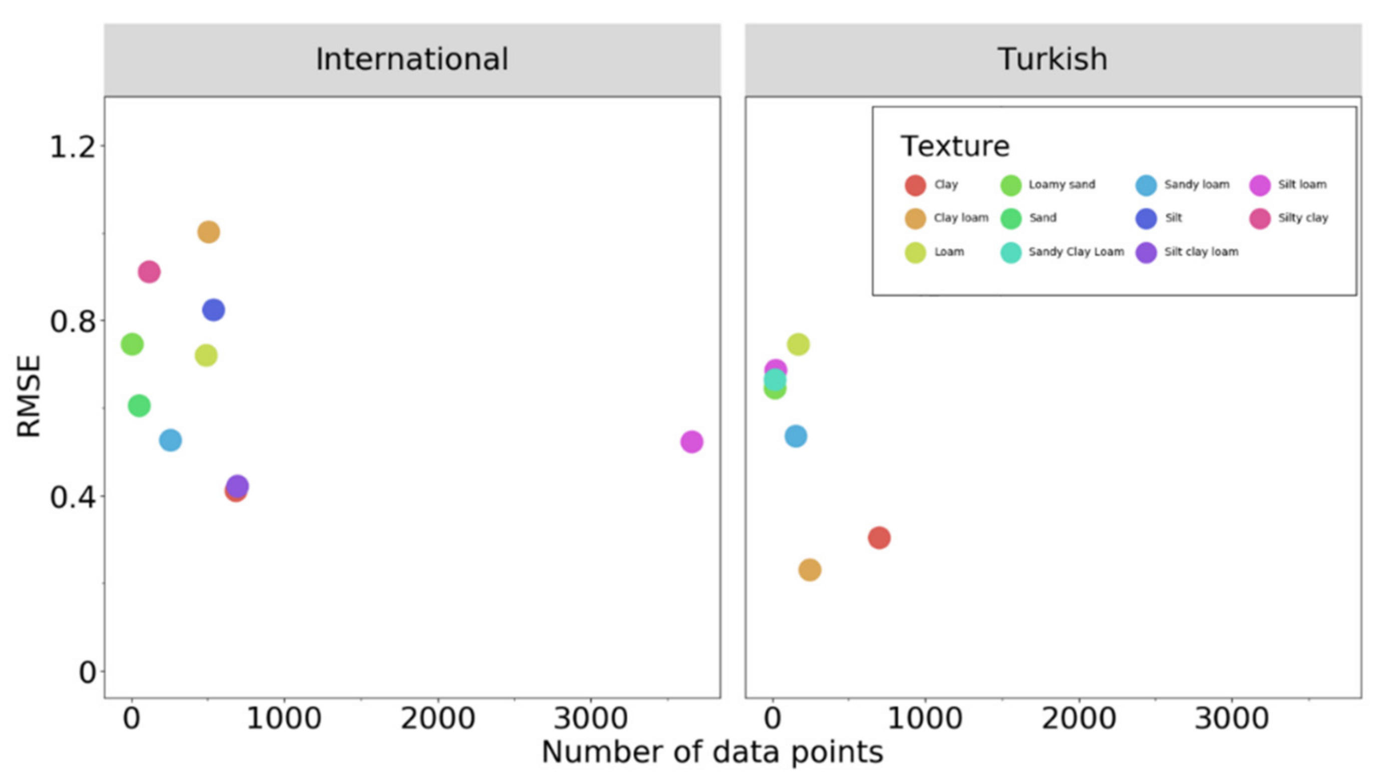
3.2. Performance across Soil Textures
3.3. Performance at the Wet, Intermediate and Dry Parts of the SHCC
4. Discussion
4.1. Accuracy and Reliability of the Developed PTFs
4.2. Importance of Input Variables
4.3. Performance across Textural Classes and Tension Ranges
5. Conclusions
Author Contributions
Funding
Institutional Review Board Statement
Informed Consent Statement
Data Availability Statement
Conflicts of Interest
References
- Bouma, J. Using Soil Survey Data for Quantitative Land Evaluation. In Advances in Soil Science; Stewart, B., Ed.; Springer: New York, NY, USA, 1989; Volume 9, ISBN 978-1-4612-3532-3. [Google Scholar]
- Vereecken, H.; Schnepf, A.; Hopmans, J.W.; Javaux, M.; Or, D.; Roose, T.; Vanderborght, J.; Young, M.H.; Amelung, W.; Aitkenhead, M.; et al. Modeling Soil Processes: Review, Key Challenges, and New Perspectives. Vadose Zo. J. 2016, 15, 1–57. [Google Scholar] [CrossRef]
- Assouline, S.; Or, D. Conceptual and Parametric Representation of Soil Hydraulic Properties: A Review. Vadose Zo. J. 2013, 12. [Google Scholar] [CrossRef]
- Van Genuchten, M.T. A Closed-form Equation for Predicting the Hydraulic Conductivity of Unsaturated Soils1. Soil Sci. Soc. Am. J. 1980, 44, 892. [Google Scholar] [CrossRef]
- Mualem, Y. A new model for predicting the hydraulic conductivity of unsaturated porous media. Water Resour. Res. 1976, 12, 513–522. [Google Scholar] [CrossRef]
- Schaap, M.G.; Leij, F.J. Using neural networks to predict soil water retention and soil hydraulic conductivity. Soil Tillage Res. 1998, 47, 37–42. [Google Scholar] [CrossRef]
- Børgesen, C.D.; Iversen, B.V.; Jacobsen, O.H.; Schaap, M.G. Pedotransfer functions estimating soil hydraulic properties using different soil parameters. Hydrol. Process. 2008, 22, 1630–1639. [Google Scholar] [CrossRef]
- Parasuraman, K.; Elshorbagy, A.; Si, B.C. Estimating Saturated Hydraulic Conductivity In Spatially Variable Fields Using Neural Network Ensembles. Soil Sci. Soc. Am. J. 2006, 70, 1851–1859. [Google Scholar] [CrossRef]
- Schaap, M.G.; Leij, F.J.; van Genuchten, M.T. Neural Network Analysis for Hierarchical Prediction of Soil Hydraulic Properties. Soil Sci. Soc. Am. J. 1998, 62, 847. [Google Scholar] [CrossRef]
- Weynants, M.; Vereecken, H.; Javaux, M. Revisiting Vereecken Pedotransfer Functions: Introducing a Closed-Form Hydraulic Model. Vadose Zo. J. 2009, 8, 86–95. [Google Scholar] [CrossRef]
- Schaap, M.G.; Leij, F.J. Improved Prediction of Unsaturated Hydraulic Conductivity with the Mualem-van Genuchten Model. Soil Sci. Soc. Am. J. 2000, 64, 843–851. [Google Scholar] [CrossRef]
- Moosavi, A.A.; Sepaskhah, A. Artificial neural networks for predicting unsaturated soil hydraulic characteristics at different applied tensions. Arch. Agron. Soil Sci. 2012, 58, 125–153. [Google Scholar] [CrossRef]
- Wagner, B.; Tarnawski, V.R.; Hennings, V.; Muller, U. Evaluation of pedo-transfer functions for unsaturated soil hydraulic conductivity using an independent data set. Geoderma 2001, 102, 275–297. [Google Scholar] [CrossRef]
- Niemann, W.L.; Rovey, C.W. A systematic field-based testing program of hydraulic conductivity and dispersivity over a range in scale. Hydrogeol. J. 2009, 17, 307–320. [Google Scholar] [CrossRef]
- Bormann, H.; Klaassen, K. Seasonal and land use dependent variability of soil hydraulic and soil hydrological properties of two Northern German soils. Geoderma 2008, 145, 295–302. [Google Scholar] [CrossRef]
- Baroni, G.; Facchi, A.; Gandolfi, C.; Ortuani, B.; Horeschi, D.; Van Dam, J.C. Uncertainty in the determination of soil hydraulic parameters and its influence on the performance of two hydrological models of different complexity. Hydrol. Earth Syst. Sci. 2010, 14, 251–270. [Google Scholar] [CrossRef]
- Fodor, N.; Sándor, R.; Orfanus, T.; Lichner, L.; Rajkai, K. Evaluation method dependency of measured saturated hydraulic conductivity. Geoderma 2011, 165, 60–68. [Google Scholar] [CrossRef]
- Haghverdi, A.; Cornelis, W.M.; Ghahraman, B. A pseudo-continuous neural network approach for developing water retention pedotransfer functions with limited data. J. Hydrol. 2012, 442–443, 46–54. [Google Scholar] [CrossRef]
- Haghverdi, A.; Öztürk, H.S.; Cornelis, W.M. Revisiting the pseudo continuous pedotransfer function concept: Impact of data quality and data mining method. Geoderma 2014, 226–227, 31–38. [Google Scholar] [CrossRef]
- Schindler, U.; Müller, L. Soil hydraulic functions of international soils measured with the Extended Evaporation Method (EEM) and the HYPROP device. Open Data J. Agric. Res. 2017, 3, 10–16. [Google Scholar] [CrossRef]
- Schindler, U.; Durner, W.; von Unold, G.; Mueller, L.; Wieland, R. The evaporation method: Extending the measurement range of soil hydraulic properties using the air-entry pressure of the ceramic cup. J. Plant Nutr. Soil Sci. 2010, 173, 563–572. [Google Scholar] [CrossRef]
- Schindler, U.; Durner, W.; von Unold, G.; Müller, L. Evaporation Method for Measuring Unsaturated Hydraulic Properties of Soils: Extending the Measurement Range. Soil Sci. Soc. Am. J. 2010, 74, 1071. [Google Scholar] [CrossRef]
- Peters, A.; Iden, S.C.; Durner, W. Revisiting the simplified evaporation method: Identification of hydraulic functions considering vapor, film and corner flow. J. Hydrol. 2015, 527, 531–542. [Google Scholar] [CrossRef]
- Peters, A.; Durner, W. Simplified evaporation method for determining soil hydraulic properties. J. Hydrol. 2008, 356, 147–162. [Google Scholar] [CrossRef]
- Bezerra-Coelho, C.R.; Zhuang, L.; Barbosa, M.C.; Soto, M.A.; Van Genuchten, M.T. Further tests of the HYPROP evaporation method for estimating the unsaturated soil hydraulic properties. J. Hydrol. Hydromech. 2018, 66, 161–169. [Google Scholar] [CrossRef]
- Haghverdi, A.; Öztürk, H.S.; Durner, W. Measurement and estimation of the soil water retention curve using the evaporation method and the pseudo continuous pedotransfer function. J. Hydrol. 2018, 563, 251–259. [Google Scholar] [CrossRef]
- Singh, A.; Haghverdi, A.; Öztürk, H.S.; Durner, W. Developing Pseudo Continuous Pedotransfer Functions for International Soils Measured with the Evaporation Method and the HYPROP System: I. The Soil Water Retention Curve. Water 2020, 12, 3425. [Google Scholar] [CrossRef]
- Schindler, U.; Mueller, L.; von Unold, G.; Durner, W.; Fank, J. Emerging Measurement Methods for Soil Hydrological Studies. In Novel Methods for Monitoring and Managing Land and Water Resources in Siberia; Springer: Cham, Switzerland, 2016; pp. 345–363. ISBN 978-3-319-24409-9. [Google Scholar]
- Tranter, G.; McBratney, A.B.; Minasny, B. Using distance metrics to determine the appropriate domain of pedotransfer function predictions. Geoderma 2009, 149, 421–425. [Google Scholar] [CrossRef]
- Yang, H.; Khoshghalb, A.; Russell, A.R. Fractal-based estimation of hydraulic conductivity from soil-water characteristic curves considering hysteresis. Geotech. Lett. 2014, 4, 1–10. [Google Scholar] [CrossRef]
- Marquardt, D.W. An Algorithm for Leat-Squares Estimation of Nnonlinear Parameters. J. Soc. Indust. Appl. Math. 1963, 11, 431–441. [Google Scholar] [CrossRef]
- Morbidelli, R.; Saltalippi, C.; Cifrodelli, M. In situ measurements of soil saturated hydraulic conductivity: Assessment of reliability through rainfall—runoff experiments. Hydrol. Process. 2017, 3084–3094. [Google Scholar] [CrossRef]
- Stolte, J.; Freijer, J.I.; Bouten, W.; Dirksen, C.; Halbertsma, J.M.; Van Dam, J.C.; Van den Berg, J.A.; Veerman, G.J.; Wösten, J.H.M. Comparison of Six Methods To Determine Unsaturated Soil Hydraulic Conductivity. Soil Sci. Soc. Am. J. 1994, 58, 1596–1603. [Google Scholar] [CrossRef]
- Benson, C.H.; Gribb, M.M. Measuring unsaturated hydraulic conductivity in the laboratory and field. Geotech. Spec. Publ. 1997, 113–168. [Google Scholar]
- Durner, W.; Lipsius, K. Determining Soil Hydraulic Properties. In Encyclopedia of Hydrological Sciences; Anderson, M.G., Mcdonnell, J., Eds.; John Wiley & Sons, Ltd.: Chichester, UK, 2005; Volume 2, pp. 1121–1144. [Google Scholar]
- Cosby, B.J.; Hornberger, G.M.; Clapp, R.B.; Ginn, T.R. A Statistical Exploration of the Relationships of Soil Moisture Characteristics to the Physical Properties of Soils. Water Resour. Res. 1984, 20, 682–690. [Google Scholar] [CrossRef]
- Wösten, J.H.M.; Lilly, A.; Nemes, A.; Le Bas, C. Development and use of a database of hydraulic properties of European soils. Geoderma 1999, 90, 169–185. [Google Scholar] [CrossRef]
- Zhang, Y.; Schaap, M.G. Estimation of saturated hydraulic conductivity with pedotransfer functions: A review. J. Hydrol. 2019, 575, 1011–1030. [Google Scholar] [CrossRef]
- Minasny, B.; Hopmans, J.W.; Harter, T.; Eching, S.O.; Tuli, A.; Denton, M.A. Neural Networks Prediction of Soil Hydraulic Functions for Alluvial Soils Using Multistep Outflow Data. Soil Sci. Soc. Am. J. 2004, 68, 417–429. [Google Scholar] [CrossRef]
- Romero-Ruiz, A.; Linde, N.; Keller, T.; Or, D. A Review of Geophysical Methods for Soil Structure Characterization. Rev. Geophys. 2018, 56, 672–697. [Google Scholar] [CrossRef]
- Hao, M.; Zhang, J.; Meng, M.; Chen, H.Y.H.; Guo, X.; Liu, S.; Ye, L. Impacts of changes in vegetation on saturated hydraulic conductivity of soil in subtropical forests. Sci. Rep. 2019, 9, 1–9. [Google Scholar] [CrossRef]


| International Data (150 Soil Samples with 6963 Data Pairs) | Turkish Data (79 Soil Samples with 1340 Data Pairs) | |||||
|---|---|---|---|---|---|---|
| Attribute | Mean | Range | SD | Mean | Range | SD |
| Clay (%) | 20.0 | 0.0–60.0 | 12.5 | 34.1 | 9.4–62.2 | 15.1 |
| Silt (%) | 56.4 | 0.2–86.8 | 17.1 | 30.7 | 5.2–57.6 | 8.7 |
| Sand (%) | 23.6 | 3.9–99.8 | 17.4 | 35.3 | 6.0–84.0 | 17.4 |
| Bulk density (g cm−3) | 1.3 | 0.6–1.7 | 0.2 | 1.0 | 0.7–1.3 | 0.1 |
| Organic matter content (%) | 3.1 | 0.0–12.0 | 2.5 | 1.2 | 0.0–3.1 | 0.6 |
| Model | Input Attributes |
|---|---|
| 1 | SSC, BD, SOM, pF |
| 2 | SSC, pF |
| 3 | SSC, BD, pF |
| 4 | SSC, SOM, pF |
| Scenario | Data Sets |
|---|---|
| S1 | Training: International, Test: International. |
| S2 | Training: Turkish, Test: Turkish. |
| S3 | Training: International, Test: Turkish. |
| S4 | Training: International + Turkish, Test: Turkish. |
| Training and Test: I | Training and Test: T | Training: I.; Test: T | Training: I + T; Test: T | |||||||||||||
|---|---|---|---|---|---|---|---|---|---|---|---|---|---|---|---|---|
| M | RMSE | MAE | MBE | R | RMSE | MAE | MBE | R | RMSE | MAE | MBE | R | RMSE | MAE | MBE | R |
| 1 | 0.571 | 0.428 | 0.013 | 0.855 | 0.343 | 0.227 | 0.023 | 0.959 | 1.097 | 0.971 | −0.959 | 0.935 | 0.429 | 0.312 | −0.139 | 0.947 |
| 2 | 0.520 | 0.406 | 0.027 | 0.881 | 0.317 | 0.217 | 0.011 | 0.965 | 1.317 | 1.254 | −1.249 | 0.954 | 0.613 | 0.456 | −0.335 | 0.906 |
| 3 | 0.547 | 0.418 | 0.033 | 0.868 | 0.336 | 0.219 | 0.017 | 0.961 | 1.235 | 1.142 | −1.133 | 0.942 | 0.453 | 0.308 | −0.165 | 0.938 |
| 4 | 0.529 | 0.417 | 0.022 | 0.877 | 0.350 | 0.243 | 0.043 | 0.958 | 1.243 | 1.144 | −1.132 | 0.943 | 0.554 | 0.400 | −0.280 | 0.920 |
| Data Sets | Texture | RMSE | MAE | MBE | R |
|---|---|---|---|---|---|
| Training: I; Test: I | SiL | 0.517 | 0.421 | 0.026 | 0.881 |
| L | 0.612 | 0.485 | −0.180 | 0.789 | |
| SiCL | 0.433 | 0.342 | 0.144 | 0.870 | |
| CL | 1.124 | 0.748 | 0.288 | 0.603 | |
| SL | 0.593 | 0.522 | 0.042 | 0.700 | |
| Training: T, Test: T | C | 0.252 | 0.174 | 0.006 | 0.978 |
| SL | 0.366 | 0.277 | −0.096 | 0.966 | |
| CL | 0.206 | 0.146 | 0.018 | 0.982 | |
| L | 0.395 | 0.312 | −0.048 | 0.926 | |
| Training: I, validation: T | C | 0.986 | 0.863 | −0.860 | 0.961 |
| SL | 1.353 | 1.241 | −1.223 | 0.96 | |
| CL | 0.964 | 0.894 | −0.894 | 0.978 | |
| L | 1.444 | 1.377 | −1.370 | 0.917 | |
| Training: I and T, Test: T | C | 0.303 | 0.218 | −0.013 | 0.972 |
| SL | 0.535 | 0.446 | −0.317 | 0.963 | |
| CL | 0.230 | 0.173 | −0.094 | 0.985 | |
| L | 0.745 | 0.683 | −0.614 | 0.915 |
| Training and Test: I | Training and Test: T | Training: I, Validation: T | Training: I and T, Test: T | |||||||||
|---|---|---|---|---|---|---|---|---|---|---|---|---|
| Wet | Mid | Dry | Wet | Mid | Dry | Wet | Mid | Dry | Wet | Mid | Dry | |
| RMSE | 0.548 | 0.570 | 0.603 | 0.588 | 0.317 | 0.375 | 2.285 | 1.002 | 0.466 | 0.757 | 0.400 | 0.396 |
| MAE | 0.420 | 0.440 | 0.381 | 0.471 | 0.206 | 0.298 | 2.158 | 0.936 | 0.342 | 0.602 | 0.291 | 0.322 |
| MBE | −0.060 | 0.007 | 0.140 | 0.031 | 0.016 | 0.109 | −2.158 | −0.926 | −0.292 | −0.520 | −0.134 | 0.154 |
| R | 0.509 | 0.640 | 0.522 | 0.809 | 0.860 | 0.831 | 0.768 | 0.785 | 0.860 | 0.805 | 0.791 | 0.818 |
Publisher’s Note: MDPI stays neutral with regard to jurisdictional claims in published maps and institutional affiliations. |
© 2021 by the authors. Licensee MDPI, Basel, Switzerland. This article is an open access article distributed under the terms and conditions of the Creative Commons Attribution (CC BY) license (http://creativecommons.org/licenses/by/4.0/).
Share and Cite
Singh, A.; Haghverdi, A.; Öztürk, H.S.; Durner, W. Developing Pseudo Continuous Pedotransfer Functions for International Soils Measured with the Evaporation Method and the HYPROP System: II. The Soil Hydraulic Conductivity Curve. Water 2021, 13, 878. https://doi.org/10.3390/w13060878
Singh A, Haghverdi A, Öztürk HS, Durner W. Developing Pseudo Continuous Pedotransfer Functions for International Soils Measured with the Evaporation Method and the HYPROP System: II. The Soil Hydraulic Conductivity Curve. Water. 2021; 13(6):878. https://doi.org/10.3390/w13060878
Chicago/Turabian StyleSingh, Amninder, Amir Haghverdi, Hasan Sabri Öztürk, and Wolfgang Durner. 2021. "Developing Pseudo Continuous Pedotransfer Functions for International Soils Measured with the Evaporation Method and the HYPROP System: II. The Soil Hydraulic Conductivity Curve" Water 13, no. 6: 878. https://doi.org/10.3390/w13060878
APA StyleSingh, A., Haghverdi, A., Öztürk, H. S., & Durner, W. (2021). Developing Pseudo Continuous Pedotransfer Functions for International Soils Measured with the Evaporation Method and the HYPROP System: II. The Soil Hydraulic Conductivity Curve. Water, 13(6), 878. https://doi.org/10.3390/w13060878