Abstract
Actual evapotranspiration (ETa) estimations in arid regions are challenging because this process is highly dynamic over time and space. Nevertheless, several studies have shown good results when implementing empirical regression formulae that, despite their simplicity, are comparable in accuracy to more complex models. Although many types of regression formulae to estimate ETa exist, there is no consensus on what variables must be included in the analysis. In this research, we used machine learning algorithms—through implementation of empirical linear regression formulae—to find the main variables that control daily and monthly ETa in arid cold regions, where there is a lack of available ETa data. Meteorological data alone and then combined with remote sensing vegetation indices (VIs) were used as input in ETa estimations. In situ ETa and meteorological data were obtained from ten sites in Chile, Australia, and the United States. Our results indicate that the available energy is the main meteorological variable that controls ETa in the assessed sites, despite the fact that these regions are typically described as water-limited environments. The VI that better represents the in situ ETa is the Normalized Difference Water Index, which represents water availability in plants and soils. The best performance of the regression equations in the validation sites was obtained for monthly estimates with the incorporation of VIs (R2 = 0.82), whereas the worst performance of these equations was obtained for monthly ETa estimates when only meteorological data were considered. Incorporation of remote-sensing information results in better ETa estimates compared to when only meteorological data are considered.
1. Introduction
Arid and semi-arid regions cover approximately 41% of the world’s land and are inhabited by more than 2500 million people [1]. These regions are expected to expand because of unsustainable land and water use, as well as a result of climate change, which is exacerbating desertification [1]. In this context, an accurate quantification of evapotranspiration (ET), a relevant hydrological process in arid regions, is important for managing water resources to ensure their availability for human and environmental needs [2,3,4]. Although there have been many efforts to quantify actual evapotranspiration (ETa) in arid regions [5], few ETa direct observations exist in cold desert climates (also known as arid cold regions). For instance, from a total of 267 sites in the FLUXNET 2015 dataset, only seven sites located in arid cold regions have more than one year of records [6]. This lack of data hinders the understanding of the main processes that drive ET in these environments. Hence, the motivation of this work is to further explore if ETa in arid cold regions is driven by similar or different variables than other climates. Broadly speaking, ETa is mainly driven by energy exchange and water availability, but there are plenty of meteorological and vegetational characteristics that influence it and make its estimations more complex [7,8]. Major challenges in ETa estimation are those that make the process even more dynamic over time and variable in space. For example, when water is a limiting factor, plants decrease their transpiration through physiological adaptations such as stomata closure. Furthermore, regional advection can bring additional energy to the system, resulting in higher ETa rates that can even exceed potential ET [8]. As arid lands are vastly different from irrigated farms, typically having native vegetation with high resistance to transpiration and low ground cover, traditional ETa estimation methods are not suitable for these environments. The most common approach to determine ETa is the crop coefficient method, in which ETa is estimated from the reference evapotranspiration (ETo), computed from the Penman–Monteith formula [7] and using a crop coefficient (Kc), i.e., ETa = Kc × ETo, where Kc represents four effects that distinguish the crop from reference grass: aerodynamic resistance, albedo, surface resistance, and soil evaporation [7,8]. Nonetheless, it has been demonstrated that the crop coefficient method in general is not suitable for determining ETa of native vegetation adapted to arid conditions, because transpiration is overestimated when plants encounter suboptimal conditions of soil water as a result of not considering stomatal regulation and plant adaptations to drought [9]. Only in few exceptions has the crop coefficient method been suitable to estimate ETa in crops cultivated in arid or semi-arid regions [10,11].
Remote sensing methods have been developed to estimate ETa and have been positioned as the only feasible approach for wide areas of mixed landscapes, allowing for an improvement in water balance estimations over basin and regional scales [12,13,14,15]. One of the most used operational global ETa satellite products is MOD16, which is based on Moderate Resolution Imaging Spectroradiometer (MODIS) information. Moreover, the Satellite Application Facility on Land Surface Analysis (LSA-SAF) is widely used, but it only covers Europe, Africa, and most of South America [16,17]. Hu et al. [16] demonstrated that LSA-SAF has a better performance than MOD16, but neither products capture ETa in water-limited regions. ETa data can also be obtained from the Agricultural Research Service of the United States Department of Agriculture (USDA-ARS) ET dataset, and the data provided from the European Centre for Medium-Range Weather Forecasts (ECMWF) or the Global Land Data Assimilation System (GLDAS) models [18,19]. However, their spatial resolutions are even coarser than that of the MOD16 and LSA-SAF datasets [17]. In 2019, the European Space Agency (ESA) released the Sen-ET open-source software application for ETa modeling at high (tens of meters) and medium (1 km) spatial resolutions, and at a temporal resolution of ~5 to 10 days. The Sen-ET software uses observations of Sentinel-2 and Sentinel-3 for field-scale applications. The first validation procedure in latent heat flux was performed in the Skjern river basin (Denmark) and resulted in a correlation of 0.76 when comparing data obtained from three eddy covariance flux towers, with the best performance estimated in croplands [17]. The most common remote sensing ETa approaches are based on the surface energy balance (SEB) equation, where sensible heat (H) is estimated using land surface temperature (LST) derived from thermal infrared (TIR) sensor on satellites [12]. Although these methods have been cataloged as operational, there are difficulties on their implementation: small errors in the estimation of the LST translate into large errors in H estimates, and only few sensors offer open source TIR data [12,20].
Vegetation index (VI)-based methods to estimate ETa were developed to take advantage of remote sensing, avoiding the disadvantages associated with the methods based on SEB. VIs were developed for vegetation monitoring due to spectral reflectance signature revealing information about the state, biogeochemical composition, and structure of a leaf and canopy, but VIs can also provide information about water and carbon cycles [21]. ETa estimation methods based on VIs depend on an estimate of the density of green vegetation over the landscape, as measured by VIs or related products that combine the VIS and IR bands [12]. For example, the Normalized Difference Vegetation Index (NDVI) captures the contrast in light reflection from green leaves between the red and near infrared (NIR) bands, because red light is strongly absorbed by chlorophyll and nearly all the NIR is transmitted [22], whereas the Normalized Difference Water Index (NDWI) is sensitive to other properties, e.g., leaf water content [23], and it is also capable of representing both canopy and soil water content [24]. Thus, it is able to represent plant water stress [25]. VIs have several advantages for use in ETa algorithms: they are available from multiple sensors, and they usually change on time scales of weeks to months, so it is feasible to interpolate VI values with observations obtained several days apart, especially if they represent the activity of the vegetation. In addition, VI methods are usually simple and resilient in the presence of data gaps [4]. Moreover, VIs have been applied to natural ecosystems and achieved good results [26,27].
Several studies have demonstrated the potential of combining site-specific ETa data with remotely sensed and meteorological parameters to develop empirical models based on statistical correlations for regional-scale ETa estimates [3,12,14,15,28]. Despite their simplicity, empirical regression formulae can produce ETa values that are comparable in accuracy to more complex models, without as much computational requirements for specific expertise [4]. However, the estimation of ETa with a higher degree of accuracy and over extended time scales has forced researchers to look for techniques such as machine learning [28,29,30,31,32,33,34,35,36]. Elbeltagi et al. [37] applied five machine learning techniques to develop the Combined Terrestrial Evapotranspiration Index. Zhao et al. [30] constructed a physics-constrained machine learning model to estimate ETa, which conserves the surface energy balance and successfully reproduces extreme values. Torres et al. [29] forecasted potential ET using the multivariate relevance vector machine and limited climatic data. Granata [28] provides some examples of machine learning applications in hydrology and mentions some investigations related to ETa. However, he states that these investigations are limited and that the knowledge on the topic is still partial and fragmented. Moreover, studies that use empirical regression formulae and basic machine learning concepts usually focus on the form of the formulae that predict ETa instead of the factors that drive ETa [4,20].
The aim of this research is to investigate the main variables that control ETa in arid cold regions through implementation of empirical regression formulae using machine learning algorithms. The machine learning algorithms, based on the exhaustive feature selection (EFS) approach, which has not been used before in ETa applications, were formulated first with meteorological data and then with remote sensing data. Consequently, a secondary objective of this work is to analyze if the inclusion of remote sensing data improves ETa estimations. The scope of this work is restricted to spatial extents within the field and landscape scales (between a few hundred and a few thousand square meters) and in arid cold regions, as our review revealed that these locations are underrepresented in the scientific literature.
2. Materials and Methods
2.1. Study Sites
In this study, we used 10 sites located around the world that, according to the Köeppen climate classification system, correspond to arid cold climate (BSk and BWk) [38]. Arid cold climates are characterized by little precipitation with warm/dry summers and cold/dry winters, as opposed to hot desert climates. Arid cold climates have an annual average temperature below 18 °C, and a threshold that depends on both precipitation and temperature is used to define a region as an arid cold climate [38]. Three of the study sites are located in the Chilean Altiplano, two in Australia, and five in the United States. Figure 1 presents the location of the study sites, and Table 1 shows their main characteristics. Chilean sites are classified as desert cold climates, while the other sites are cold steppe. Additionally, the Chilean sites are located above 4000 m ASL, whereas the sites in Australia and United States are located between 125 and 1530 m ASL. The study sites represent different ecosystems of arid cold environments, which include grasslands, savannah, and shrubland (see Appendix A for a general description of the sites).

Figure 1.
(a) Location of study sites, where red stars correspond to the sites used to validate actual evapotranspiration (ETa) estimates. The bottom of the figure shows pictures of the environment of the study sites; (b) CH-AT1 [51], (c) CH-AT2 [51], (d) CH-AT3 [51], (e) AU-Cpr [48], (f) AU-Ync [49], (g) US-Cop [40], (h) US-SRG [42,52], (i) US-SRM [43,53], (j) US-Whs [44,54] , and (k) US-Wkg [45]. The latitude, longitude, and elevation of each study site are presented in Table 1.

Table 1.
Site name, location (latitude and longitude), elevation, International Geosphere-Biosphere Programme (IGBP) land cover classification, and mean annual precipitation and temperature of the study sites. The country of each site is coded as follows: Chile (CH), Australia (AU), and the United States (US).
2.2. ETa Fluxes and Meteorological Data
Actual evapotranspiration data in the Chilean sites were obtained from three eddy covariance systems (IRGASON, Campbell Sci., Utah, United States), each one having a meteorological station that allowed measuring net radiation (Rn) (CNR4, Kipp & Zonen, The Netherlands), soil heat flux (G) (HFP01SC, Hukseflux, The Netherlands), precipitation (PPT) (TE525, Campbell Sci., Logan, UT, USA), atmospheric pressure (P) (PTB110, Vaisala, Helsinki, Finland), air temperature (T) and relative humidity (RH) (CS215, Campbell Sci., Logan, UT, USA), soil temperature (Ts) (TCAV, Campbell Sci., Logan, UT, USA), and soil’s volumetric water content (VWC) (CS655, Campbell Sci., Logan, UT, USA). Vapor pressure deficit (VPD) was estimated using the previous meteorological data, and the wind speed (WS) in these sites was calculated using the measurements of the eddy covariance sonic anemometer. On the other hand, the data from Australia and the United States were obtained from the FLUXNET 2015 dataset [5,39,40,41,42,43,44,45]. The sampling frequency of the data was 30 min in all sites, which was then integrated into hourly, daily, and monthly timescales. The processing/correction methods of the eddy covariance data of all the sites are described in detail in [5,30,46,47,48,49,50]. Briefly, the following data filtering methods were applied: (i) only high-quality infilled data were chosen; (ii) ETa data samples collected in rainy periods were removed; and (iii) daytime data were utilized to avoid stable boundary layer conditions. Moreover, ETo was estimated in each site with the Penman–Monteith equation [7]. Table 2 presents the period where the data were collected in each site as well as the height at which the ETa measurements were performed.
Table 2.
Period of measurements, sensor height, dominant vegetation type, and approximate vegetation height of each site [39,40,41,42,43,44,45,51]. The country of each site is coded as follows: Chile (CH), Australia (AU), and the United States (US).
To incorporate the remote sensing data, as described below, it is important to estimate the footprint of the ETa measurements. Here, we approximated the footprint to a circle whose radius corresponds to the position of the footprint peak, xmax, following the Schuepp et al. [55] approach:
where u is the average wind speed (m/s), u∗ is the average friction velocity (m/s), z is the measuring height (m), d is the displacement height (m), and k is the von Kármán constant [56]. The footprint in each site was calculated using the sampling frequency of the data, i.e., 30 min, and then aggregating the footprint at a monthly level [57]. This approximation was chosen instead of a more complex approach, such as the Kljun et al. [57] model, for one principal reason: the required information for more complex footprint models is not available in the FLUXNET dataset, e.g., the crosswind distance standard deviation (σy) [57]. The performance of the Schuepp et al. [55] approximation was assessed by comparing the area and VI values obtained with this model and with the 80% flux footprint calculated with the Kljun et al. [57] approach in the Chilean sites, where all the required information was available (Figure 2). Note that this approach has recently been used to investigate landscape transformation processes in urban areas located in arid regions [58].

Figure 2.
(a) Example of footprint calculation with the Schuepp et al. [55] and the Kljun et al. [57] approaches. The monthly footprint was calculated at CH-AT3 in November 2019. The Kljun et al. [57] approach results in a series of consistent footprints throughout the year. The Schuepp et al. [55] approach estimate the monthly footprint as a circle. (b) Wind rose for November 2019 at CH-AT3, which determines the trend of the Kljun et al. [57] footprint.
2.3. Remote Sensing and Vegetation Indices
Reflectance images were obtained from the Level-2 science products of the Landsat 7 satellite mission and then analyzed via Google Earth Engine [59] to estimate different VIs to be incorporated into the ETa estimates. Every selected image corresponded to the less cloudy image of each month.
For every selected image, the following VIs were calculated: the NDVI, the Soil Adjusted Vegetation Index (SAVI), the Enhanced Vegetation Index (EVI), the NDWI, and the Normalized Difference Greenness Index (NDGI). Then, the average of each VI was obtained in the footprint area approximated by the Schuepp et al. [55] approach described above. These VIs were selected as they are easy to implement, and they correctly represent the vegetation state over time periods of weeks, months, and years [60]. The main disadvantages of these VIs are that (i) they have shown errors when used in bare soils; (ii) they do not have a physical meaning, which complicates a direct comparison between VI among different sites; and (iii) they are not good at representing stress effects on vegetation in the short term (hours to days) [27,60].
2.3.1. Normalized Difference Vegetation Index (NDVI)
The NDVI is the most utilized VI because it is strongly correlated with several biophysical characteristics and physiological processes of plants, including ETa [22]. The NDVI ranges between −1 and 1, where negative values correspond to water pixels, positives values but near 0 correspond to bare soil, and values near 1 are related to dense canopy. The NDVI is calculated as [12,22].
where ρNIR corresponds to the reflectance of the NIR band (0.77–0.90 μm) and ρRED (0.63–0.69 μm) is the reflectance of the visible red band. As the flux footprint areas are located at latitudes lower than 40° and have steepness lower than 5°, topographic illumination bias in the NDVI is expected to be negligible [61].
2.3.2. Soil-Adjusted Vegetation Index (SAVI)
The SAVI is a VI derived from the NDVI that includes a correction factor L, which minimizes the variations produced by the soil presence in heterogeneous surfaces. This index is calculated as [22].
The optimal value of L decreases as vegetation cover increases, i.e., L = 1 when the density is low, L = 0.5 for intermediate vegetation cover, and L = 0.25 for high density. For this investigation, L = 0.5 was used, because this value has shown good performance in reducing the noise produced by the presence of bare soil in a great range of vegetation cover densities [62].
2.3.3. Enhance Vegetation Index (EVI)
The EVI was developed to improve the sensitivity of the signal in high-biomass regions and to reduce the atmosphere influence. The EVI responds better than the NDVI to structural changes in plants and extends the range over which the NDVI responds to increases in foliage density [12,20]. The EVI is calculated as
where C1 and C2 are area correction coefficients used to account for aerosol resistance, using the blue band to correct the influence of the aerosol in the red band. ρBLUE (0.45–0.52 μm) is the reflectance of the blue band, Gf is the gain factor (set as 2.5 [22]), and Lc is the canopy background adjustment (set to 1 [22]). C1 and C2 were set as 6 and −7.5, respectively [22].
2.3.4. Normalized Difference Water Index (NDWI)
The NDWI, unlike the others VIs, focuses on identifying trends in the humidity of the studied surface, combining the water content of bare soil and vegetation. The NDWI is defined as [63].
where ρSWIR is the reflectance of the short-wave infrared (SWIR) band (1.55–1.75 µm). Ji et al. [23] suggested naming this index the Normalized Difference Infrared Index (NDII), because the NDWI was first used in MODIS, whose SWIR band is between 1.23 and 1.25 µm. However, in this study, we prefer to call it the NDWI.
2.3.5. Normalized Difference Greenness Index (NDGI)
The NDGI is a VI developed to minimize variations between background reflectance of different surfaces and to maximize the contrast between vegetation and other background components in order to prevent the effects of snow in phenology estimation [64]. The NDGI is calculated as follows [64]:
where ρGREEN is the reflectance of the green band (0.52–0.60 µm) and ε is a coefficient that depends on the satellite (ε = 0.63 for Landsat 7).
2.4. Determination of Main Variables and ETa Estimates Using Machine Learning
The general procedure to generate ETa estimates is shown in Figure 3. Remote sensing, meteorological, and flux data were used as an input in the exhaustive feature selection (EFS) algorithm [65] to determine the main variables that control ETa. The EFS algorithm selects the subset of the original features or variables that better achieves an objective, usually finding the high value of a performance metric given by an arbitrary linear regressor or classifier [65]. The EFS algorithm is the most computationally expensive feature selection method because it needs to evaluate all possible combinations of the original factors considering that only a certain amount of these should be selected [66]. However, the EFS is the optimal feature selection method as the size of the dataset and the number of required features allow this method to be computationally feasible [65]. In this research, a subset of four features was selected, and a maximum of 18 features that are typically used in ET studies were evaluated (Table 3). It was decided to use subsets of four factors because, in preliminary tests, no significant improvement in formulae performance was achieved when more factors were added.

Figure 3.
Flowchart of the methods used in this study. Remote sensing, and flux, and meteorological data were used to obtain the main variables and actual evapotranspiration (ETa) estimate formulae by the application of machine learning algorithms.
Table 3.
Variables analyzed in this study and their respective symbols and units.
A linear equation to estimate ETa was constructed using the four main variables found with the EFS algorithm:
where Vari is the main variables that explain ETa, which are found using the EFS algorithm; ai represents the regression coefficients of the linear equation. The regression coefficients were found with ordinary least squares (OLS) [67]. To identify the main variables and the regression coefficients, the input data were normalized; i.e., each one of the Vari ranged between 0 and 1. This normalization ensured that the EFS chose the main variables for their contribution to the ETa variability and not because of their magnitude. The coefficient of determination (R2) of the linear regression was chosen as the performance metric. The combination of EFS and OLS was chosen to create the ETa estimation equations instead of non-linear machine learning models like tree-base models, because linear equations allow a deeper interpretation of the results.
Data were separated into two groups: the training data (CH-AT2, CH-AT3, AU-Cpr, US-Cop, US-SRG, US-SRM, and US-Wkg) and the validation data (CH-AT1, AU-Ync, and US-Wkg). The training data were used to generate a global estimation that could fit all of the sites. The performance of this equation was evaluated with the validation data. Furthermore, site-specific formulae were constructed with the data of each site with the aim of determining the most important factors minimizing the influence of the amount of data that each of the sites has on the results. Global and site-specific equations were found for daily and monthly time scales, both with ETa expressed as mm/day, with only meteorological data. Then, VIs were incorporated in monthly estimations to evaluate the relevance of incorporating remote sensing data into estimations that consider places with different cover types but the same climate.
3. Results
3.1. Remote Sensing Information
For all the Chilean sites, a high correlation was found (coefficient of determination, R2 > 0.84 and root mean square error, RMSE < 0.17) between VI values calculated with both footprint approaches, despite the difference in the footprint areas (Table 4 and Figure 4). Moreover, when increasing xmax in more than one order of magnitude, the high correlation between VI values calculated with the Schuepp et al. [55] and the Kljun et al. [57] approaches was maintained and only decreased when the footprint reached a surface that had different characteristics. Hence, although the Schuepp et al. [55] approach may not precisely represent the footprint, it allows the estimation of VIs that agree with those calculated with a more sophisticated footprint method, such as the Kljun et al. [57] approach.
Table 4.
Comparison between vegetation index (VI) values obtained with the footprints calculated with the Kljun et al. [57] and the Schuepp et al. [55] approaches. The mean values of each VI calculated with both approaches in the study period are presented. In addition, the coefficient of determination (R2) and root mean square error (RMSE) between the results of the Kljun et al. [57] and the Schuepp et al. [55] approaches are shown.

Figure 4.
Footprint areas calculated with the Kljun et al. [57] approach and the Schuepp et al. [55] approach at a monthly level for the (a) CH-AT1, (b) CH-AT2, and (c) CH-AT3 sites.
The temporal evolution of ETa, precipitation, and VIs on the validation sites is shown in Figure 5, Figure 6 and Figure 7. At the US-Wkg validation site, ETa responded to water availability determined by the amount of precipitation (Figure 5). Additionally, the VIs responded in the same way as ETa, except for the SAVI and NDVI, whose values decreased drastically in the presence of precipitation events. This behavior is not common for all the sites. For example, at the AU-Ync validation site (Figure 6), the relationship between precipitation and ETa is weak. However, it seems that ETa responded to water availability, represented as the NDWI. Furthermore, the EVI explains some of the ETa peaks. In the CH-AT1 validation site, no relationship between the Vis and ETa was found (Figure 7), most likely because groundwater is shallow in this site. Hence, there is water available for evapotranspiration throughout the year.
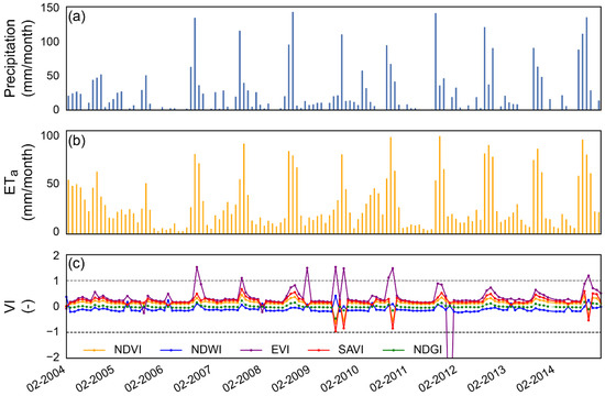
Figure 5.
Temporal evolution of monthly precipitation (a), monthly ETa (b), and monthly VIs (c) in US-Wkg.
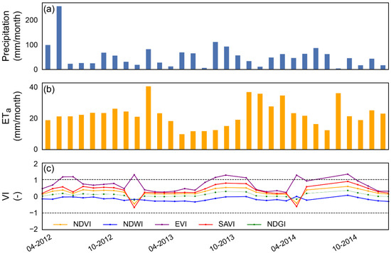
Figure 6.
Temporal evolution of monthly precipitation (a), monthly ETa (b), and monthly VIs (c) in AU-Ync.
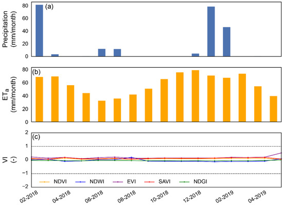
Figure 7.
Temporal evolution of monthly precipitation (a), monthly ETa (b), and monthly VIs (c) in CH-AT1.
3.2. ETa Estimation Formulae
The global and the site-specific ETa estimation formulae are presented in Table 5. The daily global equation developed with the seven sites of the training data reached an R2 of 0.60 and an RMSE of 0.64 mm/day (Figure 8a). On monthly timescales and only considering meteorological information, the global equation developed with the training sites reaches an R2 of 0.70 and an RMSE of 0.47 mm/day (Figure 8b). The monthly global equation that does include VIs reached an R2 of 0.67 and an RMSE of 0.49 mm/day (Figure 8c). In all cases, monthly estimations were more accurate than daily estimations, especially because monthly averages can mask outliers. In general, the monthly global equation that only considers meteorological information performed better than the equation that includes VIs. However, in general, the site-specific equations that include VIs resulted in better outcomes (Table 5).
Table 5.
Global and site-specific ETa estimate formulae obtained with the training data set, and their respective coefficient of determination. ETa is expressed in mm/day in all cases.
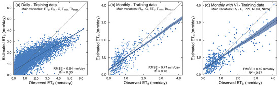
Figure 8.
Regression formulae for the training data set (including the data from the seven training sites). (a) Daily estimates; (b) monthly estimates only taking into account meteorological data; (c) monthly estimates considering meteorological data and VIs. Each panel includes the main variable selected for the construction of each formula, the RMSE, and the R2. The blue band corresponds to the 95% confidence interval.
As shown in Figure 9, in the validation sites, the best results were obtained at US-Wkg, whereas the results at CH-AT1 and AU-Ync were not satisfactory. As most of the training data came from a site located near US-Wkg, these results imply that accurate ETa estimations are obtained when the training and validation sites have similar characteristics. Figure 9 shows the R2 and RMSE values for the three validation sites. Daily estimations were usually less accurate than monthly estimates, excluding that for the AU-Ync site. Moreover, estimations that included a VI performed better than those that only considered meteorological information. The case with the best performance corresponds to the monthly estimate that includes a VI in US-Wkg (R2 of 0.82 and RMSE of 0.42 mm/day).
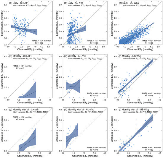
Figure 9.
Performance of the global formulae in the validation sites. CH-AT1, AU-Ync, and US-Wkg are shown from left to right. Daily, monthly, and VI monthly formulae are shown from the top to the bottom. Each panel includes the main variable selected for the construction of each formula, the RMSE, and R2. The blue band corresponds to the 95% confidence interval.
In the validation sites, only acceptable results were obtained for the US-Wkg cases, most likely because a large amount of the training data came from a site located near US-Wkg. Figure 9 shows the R2 and RMSE values for the three validation sites. Daily estimations were usually less accurate than monthly estimates, excluding that for the AU-Ync site. Additionally, estimations that include a VI performed better than those that only considered meteorological information. The case with the best performance corresponds to the monthly estimate that includes a VI in US-Wkg (R2 of 0.82 and RMSE of 0.42 mm/day).
3.3. Variables Controlling ETa
For both the daily and monthly global equations, the main variables that influence ETa, obtained as a result of applying the EFS algorithm, are Rn − G, ETo, Tmin, and Tsmax (Table 5). In both cases Rn − G is the variable that has the highest regression coefficients and, hence, is the variable that can represent better temporal evolution of ETa. Note that although ETo is among the variables that are typically used to determine ETa [10], and that it includes Rn − G, RH, VPD, and WS, it is not always among the best ranked main variables. This is most likely due to limited water availability in many of the selected study sites; hence, other variables, such as volumetric water content, could be controlling ETa. In the case where remote sensing information is used, the main variables are Rn − G, PPT, the NDGI, and the NDWI. The variable with the greatest contribution to this equation is the NDGI and that with the lowest was the Rn − G.
Table 6 shows the occurrence of the main variables found for all the sites for the site-specific equations. For the daily estimates, the most important variables are Rn − G, VWC, and ETo, which show that daily ETa depends on both energy and water availability. In the case of the monthly estimations, the main variables are Rn − G, T, and Ts. The monthly estimates that include VIs have VPD and the NDWI as the principal variables. When only meteorological information is considered, the available energy is the principal variable that explains ETa in both daily and monthly scales. In the case when remote sensing information is incorporated the main variable is NDWI, however, the available energy is still equally important as other variables that represent the availability of water, such as PPT and VPD.
Table 6.
Number of times that every variable is selected in a site-specific equation for daily, monthly, and monthly with VI estimates.
4. Discussion
A comparison of ETa estimation formulae between studies is difficult due to the many differences between them: (1) calibration and validation procedures; (2) data selection and processing; (3) temporal scale of estimates; (4) number and characteristic of the variables used; and (5) number and location of field sites considered [20]. However, in this section, the results obtained in other studies that have used regression formulae or machine learning algorithms to estimate ETa are discussed and compared to our results. Carter and Liang [4] evaluated seven regression algorithms for daily ETa estimations with meteorological and/or remote sensing data of different cover types, reaching R2 between 0.43 to 0.52 for all sites. The performance obtained by Carter and Liang [4] in the sites with climate different than arid cold desert is slightly lower than that obtained in this study for daily estimations considering the training data (R2 = 0.6). The algorithms evaluated by Carter and Liang [4] correspond to simple linear equations, such as the Yebra et al. [20] formula, and to more complex equations, such as that developed in [68] Granata [28] fitted three daily ETa estimations models that include different meteorological data with four different machine learning algorithms in a subtropical humid site located in Florida. All of them reached R2 values of over 0.92, because only one site was considered and the availability of water is not limited, as opposed to what occur in arid cold regions. However, better results were obtained in the model with a greater number of variables.
Studies in natural arid zones landscapes are scarce compared to studies performed in agricultural lands located in mesic environments. Investigations performed in the western of the U.S. have provided the basis for improved estimation of ETa in arid and semi-arid environments [2,3,27,60,69]. Bunting et al. [3] evaluated three regression equations that estimates ETa in a period of 16 days in riparian and upland sites in California. One of the equations is a multiple linear regression that includes the MODIS EVI and precipitation data (R2 = 0.74). Nagler et al. [2,27] developed two different regression equations that require meteorological and MODIS EVI information to estimate ETa in riparian environments of the Colorado, Rio Grande, and San Pedro rivers in Colorado, U.S. Both equations are based on the relationship between the leaf area index (LAI) and light absorption by the canopy, and the linear relationship between the EVI and LAI. Both equations have good predictive capability (R2 = 0.73 and 0.74, respectively). Performances of the best results obtained in this research are comparable to the studies reviewed.
In our work, different arid cold climate sites were used to generate linear regression formulae to estimate ETa. Although other works show better results in sites that only have the same vegetation cover [20], we obtained very different performances in daily, monthly, and monthly with VIs estimations in the validation sites with similar vegetation cover, such as in the case of AU-Ync and US-Wkg (R2 = 0.03, 0.00, 0.16 and R2 = 0.69, 0.78, 0.82, respectively). In regard to this, note that the linear formulation of the regression formulae should not be an important source of error, as Carter and Liang [4] demonstrated that different regression formulae, with different theoretical bases and the same input data, have similar performance.
According to Allen et al. [7], the main meteorological variables affecting ETa are radiation, air temperature, air humidity, and wind speed. Several investigations have studied the relative importance of these variables in ETa processes in arid regions. However, these studies generally focus on the behavior of ETo instead of ETa, so they do not consider the effects of water stress. For example, Adnan et al. [70] and Eslamian et al. [71] studied the influence of meteorological variables on ETo estimations in semi-arid, arid, and hyper-arid climates (Pakistan and Iran) using the Penman–Monteith formulation. Both studies concluded that air temperature and humidity are the most important meteorological variables affecting ETo. One of the few studies that analyze the sensitivity of ETa estimations to variations in meteorological and remote sensing data in a semi-arid region is that conducted by Mokhtari et al. [72]. They analyzed the sensitivity of METRIC (mapping evapotranspiration at high resolution with internalized calibration) and concluded that it is highly sensitive to surface temperature, net radiation, and air temperature, and it is less sensitive to the LAI, SAVI, and WS (except for WS at low level of vegetation cover). Our results indicate that available energy is the main variable that controls ETa, which agrees with previous studies that investigated ETa components in as many climate and vegetation cover types as possible [4,73,74,75]. For example, Wang et al. [73] correlated ETa measurements with radiation, air, and land surface temperature, the EVI and NDVI, and soil moisture. They concluded that correlation coefficients between Rn and ETa are the highest, followed by Ts and VIs.
In this research, of the four most important meteorological variables, only wind speed was not decisive in estimating ETa in all of the cases studied. This fact agrees with the findings of Granata [28], who proved that it is possible to generate accurate and precise estimates of daily ETa through machine learning algorithms only with mean temperature, net solar radiation, and relative humidity data, pointing out that the incorporation of wind speed does not improve the ETa estimations compared to the case when it is not accounted for. However, he analyzed ETa in a subtropical humid climate, where the number of sunshine hours is considered to be the more dominant variable as opposed to arid climates, where wind speed is an important variable [46]. Irmak et al. [76] compared 11 ETa models in a crop field in Nebraska, USA, to study their complexity on hourly, daily, and seasonal scales. They concluded that wind speed, and other meteorological variables such as temperature, gained importance in daily and hourly calculations, while on seasonal scales, radiation was the dominant variable. As shown in these studies, it was expected that wind speed would be an important variable in daily ETa estimations. However, the method and the number of variables chosen in this research could mask its effects: EFS selects the most important meteorological variable or variables that explain ETa, in this case Rn − G and the NDWI, accompanied by variables whose unique objective is to make the equation work numerically; furthermore, the WS influence could be well represented in ETo, so Rn − G, VWC, and Ts are variables that provide more information about ETa variability than WS itself. In arid regions, WS plays an important role when advection of dry air enhances evaporation and affects the energy balance by horizontal transport of latent heat [46,77].
Our findings support that regardless of the climate type, atmospheric demand and available energy determine ETa when water supply is sufficient, whereas soil moisture becomes an important factor controlling ETa when soil water supply is deficient [75]. Bunting et al. [3] proved that ETa estimations in semi-arid upland sites using multiple linear regression improve with the incorporation of a moisture input. However, variables such as precipitation and soil moisture are not usually used as the moisture input for several reasons: (1) surface precipitation and soil moisture measurements are point measurements, limiting the possibilities for upscaling; (2) a lag effect must be considered with precipitation; and (3) soil moisture remote sensing products are difficult to process, and their resolution is of several kilometers [4]. In this context, we expected that few of the ETa estimation formulae presented in Table 5 would incorporate PPT and VWC in the four most important variables found by the EFS algorithm. However, a novel and non-expected result that we found when remote sensing information was added, is the appearance of the NDWI as the main variable that explains the moisture input (see ETa estimation formulae shown in Table 5). Moreover, in studies performed in climates different than arid cold deserts, NDVI and EVI are the remote sensing VIs that are typically used to determine ETa because they represent the vegetation activity [4,26,75,78]. Unlike other VIs, NDWI is capable of indicating trends in soil and vegetation wetness [25,79], so it is a valid water availability input that does not have the same disadvantages of PPT and VWC, as mentioned above. Hence, NDWI is a VI that improves the estimation of ETa in arid cold regions, and that has not received too much attention in studies conducted in other climates.
The use of remote sensing information is fundamental in estimating ETa for regional-scale and heterogeneous landscapes [12]. This research proved that the incorporation of VIs helps to extrapolate global equations to each one of the sites. However, it has been proven that VIs are not sufficient to accurately estimate ETa [20]. Carter and Liang [4] noted that, at minimum, ETa estimates with Vis require the inclusion of radiation data. However, it is recommended to increase the number of input variables. Our results demonstrate that acceptable results were achieved with four variables.
Although the contribution of the VIs to the improvement in ETa estimations at the regional level is indisputable, there are several sources of error that must be addressed. One of the most important is the influence of bare soil on the reflectance response, especially in high-resolution satellites, such as Landsat. Jarchow et al. [69,80] compared Landsat 5 and Landsat 8 EVI values to the MODIS EVI in a riparian zone of the Colorado River, Mexico, finding low correlations over bare soil and sparsely vegetated areas. Additionally, they suggest being cautious when high-resolution Landsat EVI data are analyzed over heterogeneous areas with low vegetation densities, such as those commonly encountered in cold arid and semi-arid environments, because soil presence contributes to increased variability in the response of the NIR and red bands.
The poor correlations obtained in this study between VIs and ETa could be explained by several factors. Firstly, as mentioned before, the presence of bare soil can perturb the calculation of VIs [80]. Secondly, in this research, only ETa outliers were extracted, whereas other studies selected data that accomplished some characteristics. For example, Yebra et al. [20] selected data of days where only transpiration was expected to be dominant, and Scott et al. [81] excluded data from precipitation events and outliers of meteorological variables. In the presence of important rainfall events, most of the VIs considered in this study, except for the NDWI and EVI, have negative values. The values of the VIs indicate that there should be a lower ETa rate when it rains, since they actually increase. VI values obtained in this research are different to those reported in previous studies [82,83,84]. However, they are different from each other, highlighting the importance of satellite selection.
5. Conclusions
In this study, we generated linear regression formulae to estimate daily and monthly ETa in arid cold sites. Different performances were obtained for every site, and the following trends were identified: (1) better results were obtained for monthly than for daily estimates; (2) incorporation of remote sensing information allows one to extrapolate formulae to other sites in order to obtain better results than estimations with only meteorological data; (3) the available energy is the most important meteorological variable in ETa estimations for the sites evaluated in this research; and (4) in arid regions, it is important to incorporate estimations of water availability. As precipitation and soil moisture are point measurements that do not allow one to extrapolate estimations in wide areas, the NDWI could be incorporated as a proxy for water availability in the heterogeneous landscapes located in arid cold regions. Furthermore, more studies that analyze variables controlling ETa in arid natural landscapes are needed, because ETa in drylands is exposed to different factors than in more humid environments, such as water stress, advection, and vegetation with adaptations to drought. Global ETo investigations cannot study the complexity of ETa in arid cold regions in depth.
Author Contributions
Conceptualization, J.M. and F.S.; validation and formal analysis, J.M.; both authors contributed to the methodology and writing of the manuscript; project administration, F.S.; funding acquisition, F.S. Both authors have read and agreed to the published version of the manuscript.
Funding
This research and the APC were funded by the Agencia Nacional de Investigación y Desarrollo (ANID), by grants FONDECYT/1170850, FONDECYT/1210221 and FONDEQUIP/EQM170024.
Institutional Review Board Statement
Not applicable.
Informed Consent Statement
Not applicable.
Data Availability Statement
Original hourly data from the study sites are available at http://dx.doi.org/10.17632/vkkzxkwwjk.2 [51]. The data from the Australian and United States sites are available in the FLUXNET 2015 dataset [5,39,40,41,42,43,44,45].
Acknowledgments
The authors thank the Centro de Desarrollo Urbano Sustentable (CEDEUS—ANID/FONDAP/15110020) and the Centro de Excelencia en Geotermia de los Andes (CEGA—ANID/FONDAP/15090013) for supporting this investigation.
Conflicts of Interest
The authors declare no conflict of interest and declare that the funders had no role in the design of the study; in the collection, analyses, or interpretation of data; in the writing of the manuscript, or in the decision to publish the results.
Appendix A. Sites Description
Appendix A.1. CH-AT1
This site corresponds to a riparian wetland located in the Chilean Andean plateau (22.02° S, 68.05° W, elevation: 4182 m ASL). The annual precipitation is concentrated in summer months due to the effect of the South American monsoon and is ~78 mm (2007–2016 time period), whereas the annual mean temperature is ~5.8 °C (1969–1987 time period) [85]. The area is dominated by the presence of the reed Oxychloe andina and the grass Deyeuxia sp. The Parastrephia sp. shrub and some hydrophytes, such as Lilaeopsis macloviana and Myriophyllum quitense, are also present.
Appendix A.2. CH-AT2
This site is located 1500 m north of CH-AT1 (22.01° S, 68.05° W, elevation: 4330 m ASL). Unlike the riparian wetland (CH-AT1), only grass and some shrubs are present at this site, where the dominant species is the grass Festuca genera. Because CH-AT1 and CH-AT2 are near to each other, the climate characterization of CH-AT2 is the same as in the riparian wetland.
Appendix A.3. CH-AT3
This site is in the Putana wetland, which is located in the Altiplano of the Antofagasta Region, Chile (22.52° S, 68.02° W, elevation: 4255 m ASL). The annual precipitation is ~106 mm (2008–2017 time period), also concentrated in the summer months, and the mean annual temperature is ~1.7 °C (2013–2016 time period) [85]. The presence of water in the wetland is due to contributions of the Putana River and groundwater upwelling. The vegetation in the study site is classified as perennial grassland dominated by Oxychloe andina and some grass of the Festuca and Deyeuxia genera. There are also some hydrophytes, such as Ranunculus uniflorus and Azolla filiculoides.
Appendix A.4. AU-Cpr
This study site is located 25 km north of Renmark in South Australia at Calperum Station (34.00° S, 140.59° E, elevation: ~166 m ASL). The mean annual precipitation is approximately 250 mm. More rainfall is generally expected in the cooler winter and spring periods, but occasional summer rainfall events occur. The mean annual temperature is 18 °C, ranging between −3 and 45 °C. The vegetation is dominated by several species of Eucalyptus, but also it is possible to find mid-story species belonging to Eremophila, Hakea, Olearia, Senna, and Melaleuca genera [41,83].
Appendix A.5. AU-Ync
This site is located in the Yanco study area (34.99° S, 146.29° E, elevation: ~125 m ASL), which is situated within the western plains of the Murrumbidgee River catchment, in New South Wales, Australia. Precipitation is distributed evenly across all months, reaching 419 mm per year. Daily mean temperatures vary significantly from 34 °C in January to 14.2 °C in July. The site consists of a homogeneous flat grassland that is used for the grazing of livestock. The grassland is dominated by perennial tussock grasses, such as kangaroo and wallaby grasses [86].
Appendix A.6. US-Cop
This site, named Corral Pocket, is a semiarid grassland located in southeast Utah, USA (38.09° N, 109.39° W, elevation: 1520 m ASL). Mean annual precipitation and temperature are 216 mm and 12 °C, respectively. About 33% of the precipitation occurs during summer. The vegetation is dominated by the perennial Hilaria jamesii and Stipa hymenoides bunchgrasses and the Coleogyne ramosissima shrub, with other grasses and annuals making up a small percentage of total plant cover [40].
Appendix A.7. US-SRG
This site corresponds to Santa Rita Grassland, which is located in the Santa Rita Experimental Range, 45 km south of Tucson, Arizona, USA (31.79° N, 110.83° W, elevation: 1290 m ASL). Mean annual precipitation is 377 mm. Because of the North American monsoon, about 50% of rainfall occurs during summer. The mean air temperature is 19 °C, with winter freezes in November and daytime maxima that exceed 35° in June [42,81]. This site is dominated by the South African warm season bunchgrass, Lehmann Lovegrass (Eragrostis lehmanniana), and it has a 11% cover of mesquite (Prosopis velutina) [42].
Appendix A.8. US-SRM
This site corresponds to the Santa Rita mesquite savanna site, which is also located in the Santa Rita Experimental Range, USA, 5 km from the Santa Rita Mesquite site (31.82° N, 110.87° W, elevation: 1116 m ASL). The site vegetation consists of the leguminous tree Prosopis velutina (35% of the vegetation cover) growing in a matrix of native and nonnative perennial grasses, subshrubs, and scattered succulents [81].
Appendix A.9. UC-Whs
This site corresponds to the Lucky Hills Shrubland, in the U.S. Department of Agriculture Agricultural Research Service (USDA-ARS) Walnut Gulch Experimental Watershed. It is located 80 km east of Santa Rita sites (31.74° N, 110.05° W, elevation: 1370 m ASL). Annual precipitation is lower than that in the Santa Rita sites, reaching 285 mm. The mean air temperature is also quite lower, reaching 17.6 °C. This site has a large diversity of shrubs that are typically found throughout the Sonoran and Chihuahuan Deserts, such as Parthenium incanum, Acacia constricta, Larrea tridentata, and Flourensia cernua [44].
Appendix A.10. US-Wkg
This site corresponds to the Walnut Gulch Kendall Grasslands, which is located 10 km apart of US-Whs, also in the USDA-ARS Walnut Gulch Experimental Watershed (31.74° N, 109.94° W, elevation: 1530 m ASL). In the period of 2005–2014 a mean annual temperature of 17.3 °C and an annual precipitation of 294 mm have been reported. The dominant species are Eragrostis lehmanniana, Bouteloua eripoda, and Aristida spp., all of them belonging to the Poaceae family. It is also possible to see woody species as Ephedra viridis and Artemisia filifolia [45].
References
- Gaur, M.K.; Squires, V.R. Geographic Extent and Characteristics of the World’s Arid Zones and Their Peoples. In Climate Variability Impacts on Land Use and Livelihoods in Drylands; Gaur, M.K., Squires, V.R., Eds.; Springer International Publishing: Cham, Switzerland, 2018; pp. 3–20. ISBN 978-3-319-56681-8. [Google Scholar]
- Nagler, P.L.; Scott, R.L.; Westenburg, C.; Cleverly, J.R.; Glenn, E.P.; Huete, A.R. Evapotranspiration on Western U.S. Rivers Estimated Using the Enhanced Vegetation Index from MODIS and Data from Eddy Covariance and Bowen Ratio Flux Towers. Remote Sens. Environ. 2005, 97, 337–351. [Google Scholar] [CrossRef]
- Bunting, D.P.; Kurc, S.A.; Glenn, E.P.; Nagler, P.L.; Scott, R.L. Insights for Empirically Modeling Evapotranspiration Influenced by Riparian and Upland Vegetation in Semiarid Regions. J. Arid Environ. 2014, 111, 42–52. [Google Scholar] [CrossRef]
- Carter, C.; Liang, S. Comprehensive Evaluation of Empirical Algorithms for Estimating Land Surface Evapotranspiration. Agric. For. Meteorol. 2018, 256–257, 334–345. [Google Scholar] [CrossRef]
- Pastorello, G.; Trotta, C.; Canfora, E.; Chu, H.; Christianson, D.; Cheah, Y.-W.; Poindexter, C.; Chen, J.; Elbashandy, A.; Humphrey, M.; et al. The FLUXNET2015 Dataset and the ONEFlux Processing Pipeline for Eddy Covariance Data. Sci. Data 2020, 7, 225. [Google Scholar] [CrossRef]
- FLUXNET2015 Dataset. Available online: https://fluxnet.org/data/fluxnet2015-dataset/ (accessed on 2 March 2021).
- Allen, R.G.; Pereira, L.S.; Raes, D.; Smith, M. Crop Evapotranspiration—Guidelines for Computing Crop Water Requirements—FAO Irrigation and Drainage Paper 56; Food and Agriculture Organization of the United Nations: Rome, Italy, 1998. [Google Scholar]
- Allen, R.G.; Pereira, L.S.; Howell, T.A.; Jensen, M.E. Evapotranspiration Information Reporting: I. Factors Governing Measurement Accuracy. Agric. Water Manag. 2011, 98, 899–920. [Google Scholar] [CrossRef]
- Mata-González, R.; McLendon, T.; Martin, D.W. The Inappropriate Use of Crop Transpiration Coefficients (Kc) to Estimate Evapotranspiration in Arid Ecosystems: A Review. Arid Land Res. Manag. 2005, 19, 285–295. [Google Scholar] [CrossRef]
- Elbeltagi, A.; Deng, J.; Wang, K.; Malik, A.; Maroufpoor, S. Modeling Long-Term Dynamics of Crop Evapotranspiration Using Deep Learning in a Semi-Arid Environment. Agric. Water Manag. 2020, 241, 106334. [Google Scholar] [CrossRef]
- Mulovhedzi, N.E.; Araya, N.A.; Mengistu, M.G.; Fessehazion, M.K.; du Plooy, C.P.; Araya, H.T.; van der Laan, M. Estimating Evapotranspiration and Determining Crop Coefficients of Irrigated Sweet Potato (Ipomoea Batatas) Grown in a Semi-Arid Climate. Agric. Water Manag. 2020, 233, 106099. [Google Scholar] [CrossRef]
- Glenn, E.P.; Nagler, P.L.; Huete, A.R. Vegetation Index Methods for Estimating Evapotranspiration by Remote Sensing. Surv. Geophys. 2010, 31, 531–555. [Google Scholar] [CrossRef]
- El Masri, B.; Rahman, A.F.; Dragoni, D. Evaluating a New Algorithm for Satellite-Based Evapotranspiration for North American Ecosystems: Model Development and Validation. Agric. For. Meteorol. 2019, 268, 234–248. [Google Scholar] [CrossRef]
- Srivastava, A.; Sahoo, B.; Raghuwanshi, N.S.; Singh, R. Evaluation of Variable-Infiltration Capacity Model and MODIS-Terra Satellite-Derived Grid-Scale Evapotranspiration Estimates in a River Basin with Tropical Monsoon-Type Climatology. J. Irrig. Drain. Eng. 2017, 143, 04017028. [Google Scholar] [CrossRef]
- Billah, M.M.; Goodall, J.L.; Narayan, U.; Reager, J.T.; Lakshmi, V.; Famiglietti, J.S. A Methodology for Evaluating Evapotranspiration Estimates at the Watershed-Scale Using GRACE. J. Hydrol. 2015, 523, 574–586. [Google Scholar] [CrossRef]
- Hu, G.; Jia, L.; Menenti, M. Comparison of MOD16 and LSA-SAF MSG Evapotranspiration Products over Europe for 2011. Remote Sens. Environ. 2015, 156, 510–526. [Google Scholar] [CrossRef]
- Guzinski, R.; Nieto, H. Evaluating the Feasibility of 1016Using Sentinel-2 and Sentinel-3 Satellites for High-Resolution Evapotranspiration Estimations. Remote Sens. Environ. 2019, 221, 157–172. [Google Scholar] [CrossRef]
- DHI-GRAS. User Manual for SEN-ET SNAP Plugin; DHI GRAS: Horsholm, Dnemark, 2020; Available online: https://www.esa-sen4et.org/static/media/sen-et-user-manual-v1.1.0.5d1ac526.pdf (accessed on 22 March 2021).
- Semmens, K.A.; Anderson, M.C.; Kustas, W.P.; Gao, F.; Alfieri, J.G.; McKee, L.; Prueger, J.H.; Hain, C.R.; Cammalleri, C.; Yang, Y.; et al. Monitoring Daily Evapotranspiration over Two California Vineyards Using Landsat 8 in a Multi-Sensor Data Fusion Approach. Remote Sens. Environ. 2016, 185, 155–170. [Google Scholar] [CrossRef]
- Yebra, M.; Van Dijk, A.; Leuning, R.; Huete, A.; Guerschman, J.P. Evaluation of Optical Remote Sensing to Estimate Actual Evapotranspiration and Canopy Conductance. Remote Sens. Environ. 2013, 129, 250–261. [Google Scholar] [CrossRef]
- Huete, A.R. Vegetation Indices, Remote Sensing and Forest Monitoring. Geogr. Compass 2012, 6, 513–532. [Google Scholar] [CrossRef]
- Glenn, E.P.; Neale, C.M.U.; Hunsaker, D.J.; Nagler, P.L. Vegetation Index-Based Crop Coefficients to Estimate Evapotranspiration by Remote Sensing in Agricultural and Natural Ecosystems. Hydrol. Process. 2011, 25, 4050–4062. [Google Scholar] [CrossRef]
- Ji, L.; Zhang, L.; Wylie, B.K.; Rover, J. On the Terminology of the Spectral Vegetation Index (NIR − SWIR)/(NIR + SWIR). Int. J. Remote Sens. 2011, 32, 6901–6909. [Google Scholar] [CrossRef]
- Wang, L.; Qu, J.J.; Hao, X.; Zhu, Q. Sensitivity Studies of the Moisture Effects on MODIS SWIR Reflectance and Vegetation Water Indices. Int. J. Remote Sens. 2008, 29, 7065–7075. [Google Scholar] [CrossRef]
- Sriwongsitanon, N.; Gao, H.; Savenije, H.H.G.; Maekan, E.; Saengsawang, S.; Thianpopirug, S. Comparing the Normalized Difference Infrared Index (NDII) with Root Zone Storage in a Lumped Conceptual Model. Hydrol. Earth Syst. Sci. 2016, 20, 3361–3377. [Google Scholar] [CrossRef]
- Groeneveld, D.P.; Baugh, W.M.; Sanderson, J.S.; Cooper, D.J. Annual Groundwater Evapotranspiration Mapped from Single Satellite Scenes. J. Hydrol. 2007, 344, 146–156. [Google Scholar] [CrossRef]
- Nagler, P.L.; Glenn, E.P.; Nguyen, U.; Scott, R.L.; Doody, T. Estimating Riparian and Agricultural Actual Evapotranspiration by Reference Evapotranspiration and MODIS Enhanced Vegetation Index. Remote Sens. 2013, 5, 3849–3871. [Google Scholar] [CrossRef]
- Granata, F. Evapotranspiration Evaluation Models Based on Machine Learning Algorithms—A Comparative Study. Agric. Water Manag. 2019, 217, 303–315. [Google Scholar] [CrossRef]
- Torres, A.F.; Walker, W.R.; McKee, M. Forecasting Daily Potential Evapotranspiration Using Machine Learning and Limited Climatic Data. Agric. Water Manag. 2011, 98, 553–562. [Google Scholar] [CrossRef]
- Zhao, W.L.; Gentine, P.; Reichstein, M.; Zhang, Y.; Zhou, S.; Wen, Y.; Lin, C.; Li, X.; Qiu, G.Y. Physics-Constrained Machine Learning of Evapotranspiration. Geophys. Res. Lett. 2019, 46, 14496–14507. [Google Scholar] [CrossRef]
- Alemohammad, S.H.; Fang, B.; Konings, A.G.; Aires, F.; Green, J.K.; Kolassa, J.; Miralles, D.; Prigent, C.; Gentine, P. Water, Energy, and Carbon with Artificial Neural Networks (WECANN): A Statistically Based Estimate of Global Surface Turbulent Fluxes and Gross Primary Productivity Using Solar-Induced Fluorescence. Biogeosciences 2017, 14, 4101–4124. [Google Scholar] [CrossRef]
- Chaney, N.W.; Herman, J.D.; Ek, M.B.; Wood, E.F. Deriving Global Parameter Estimates for the Noah Land Surface Model Using FLUXNET and Machine Learning. J. Geophys. Res. Atmos. 2016, 121, 13218–13235. [Google Scholar] [CrossRef]
- Jung, M.; Reichstein, M.; Bondeau, A. Towards Global Empirical Upscaling of FLUXNET Eddy Covariance Observations: Validation of a Model Tree Ensemble Approach Using a Biosphere Model. Biogeosciences 2009, 6, 2001–2013. [Google Scholar] [CrossRef]
- Ke, Y.; Im, J.; Park, S.; Gong, H. Downscaling of MODIS One Kilometer Evapotranspiration Using Landsat-8 Data and Machine Learning Approaches. Remote Sens. 2016, 8, 215. [Google Scholar] [CrossRef]
- Tramontana, G.; Jung, M.; Schwalm, C.R.; Ichii, K.; Camps-Valls, G.; Ráduly, B.; Reichstein, M.; Arain, M.A.; Cescatti, A.; Kiely, G.; et al. Predicting Carbon Dioxide and Energy Fluxes across Global FLUXNET Sites with Regression Algorithms. Biogeosciences 2016, 13, 4291–4313. [Google Scholar] [CrossRef]
- Yang, F.; White, M.A.; Michaelis, A.R.; Ichii, K.; Hashimoto, H.; Votava, P.; Zhu, A.; Nemani, R.R. Prediction of Continental-Scale Evapotranspiration by Combining MODIS and AmeriFlux Data Through Support Vector Machine. IEEE Trans. Geosci. Remote Sens. 2006, 44, 3452–3461. [Google Scholar] [CrossRef]
- Elbeltagi, A.; Kumari, N.; Dharpure, J.K.; Mokhtar, A.; Alsafadi, K.; Kumar, M.; Mehdinejadiani, B.; Ramezani Etedali, H.; Brouziyne, Y.; Towfiqul Islam, A.R.M.; et al. Prediction of Combined Terrestrial Evapotranspiration Index (CTEI) over Large River Basin Based on Machine Learning Approaches. Water 2021, 13, 547. [Google Scholar] [CrossRef]
- Kottek, M.; Grieser, J.; Beck, C.; Rudolf, B.; Rubel, F. World Map of the Köppen-Geiger Climate Classification Updated. Meteorol. Z. 2006, 259–263. [Google Scholar] [CrossRef]
- Beringer, J.; Walker, J. FLUXNET2015 AU-Ync Jaxa. Available online: https://fluxnet.org/doi/FLUXNET2015/AU-Ync (accessed on 11 February 2021).
- Bowling, D. FLUXNET2015 US-Cop Corral Pocket. Available online: https://fluxnet.org/doi/FLUXNET2015/US-Cop (accessed on 11 February 2021).
- Meyer, W.; Cale, P.; Koerber, G.; Ewenz, C.; Sun, Q. FLUXNET2015 AU-Cpr Calperum. Available online: https://fluxnet.org/doi/FLUXNET2015/AU-Cpr (accessed on 11 February 2021).
- Scott, R. FLUXNET2015 US-SRG Santa Rita Grassland. Available online: https://fluxnet.org/doi/FLUXNET2015/US-SRG (accessed on 11 February 2021).
- Scott, R. FLUXNET2015 US-SRM Santa Rita Mesquite. Available online: https://fluxnet.org/doi/FLUXNET2015/US-SRM (accessed on 11 February 2021).
- Scott, R. FLUXNET2015 US-Whs Walnut Gulch Lucky Hills Shrub. Available online: https://fluxnet.org/doi/FLUXNET2015/US-Whs (accessed on 11 February 2021).
- Scott, R. FLUXNET2015 US-Wkg Walnut Gulch Kendall Grasslands. Available online: https://fluxnet.org/doi/FLUXNET2015/US-Wkg (accessed on 11 February 2021).
- Suárez, F.; Lobos, F.; de la Fuente, A.; Vilà-Guerau de Arellano, J.; Prieto, A.; Meruane, C.; Hartogensis, O. E-DATA: A Comprehensive Field Campaign to Investigate Evaporation Enhanced by Advection in the Hyper-Arid Altiplano. Water 2020, 12, 745. [Google Scholar] [CrossRef]
- Scott, R.L.; Biederman, J.A.; Hamerlynck, E.P.; Barron-Gafford, G.A. The Carbon Balance Pivot Point of Southwestern U.S. Semiarid Ecosystems: Insights from the 21st Century Drought. J. Geophys. Res. Biogeosci. 2015, 120, 2612–2624. [Google Scholar] [CrossRef]
- TERN Monitoring Sites—Calperum. Available online: http://www.ozflux.org.au/monitoringsites/calperum/calperum_pictures.html (accessed on 11 February 2021).
- TERN Monitoring Sites—Yanco. Available online: http://www.ozflux.org.au/monitoringsites/yanco/yanco_pictures.html (accessed on 11 February 2021).
- Zhou, S.; Yu, B.; Zhang, Y.; Huang, Y.; Wang, G. Partitioning Evapotranspiration Based on the Concept of Underlying Water Use Efficiency. Water Resour. Res. 2016, 52, 1160–1175. [Google Scholar] [CrossRef]
- Mosre, J.; Suarez, F. Dataset of Actual Evapotranspiration Estimates in Arid Cold Regions Using Machine Learning Algorithms with In-Situ and Remote Sensing Data. 2021. Available online: https://repositorio.uc.cl/xmlui/bitstream/handle/11534/29294/Thesis_Josefina%20Mosre_Final.pdf (accessed on 11 February 2021).
- Scott, R. US-SRG Site. Available online: https://ameriflux.lbl.gov/sites/siteinfo/US-SRG (accessed on 11 February 2021).
- Scott, R. US-SRM Site. Available online: https://ameriflux.lbl.gov/sites/siteinfo/US-SRM#image-gallery (accessed on 11 February 2021).
- Scott, R. US-Whs: Walnut Gulch Lucky Hills Shrub. Available online: https://ameriflux.lbl.gov/sites/siteinfo/US-Whs#image-gallery (accessed on 11 February 2021).
- Schuepp, P.H.; Leclerc, M.Y.; MacPherson, J.I.; Desjardins, R.L. Footprint Prediction of Scalar Fluxes from Analytical Solutions of the Diffusion Equation. Bound. Layer Meteorol. 1990, 50, 355–373. [Google Scholar] [CrossRef]
- Leclerc, M.Y.; Foken, T. Footprints in Micrometeorology and Ecology; Springer: Berlin/Heidelberg, Germany, 2014; ISBN 978-3-642-54544-3. [Google Scholar]
- Kljun, N.; Calanca, P.; Rotach, M.W.; Schmid, H.P. A Simple Two-Dimensional Parameterisation for Flux Footprint Prediction (FFP). Geosci. Model Dev. 2015, 8, 3695–3713. [Google Scholar] [CrossRef]
- Riad, P.; Graefe, S.; Hussein, H.; Buerkert, A. Landscape Transformation Processes in Two Large and Two Small Cities in Egypt and Jordan over the Last Five Decades Using Remote Sensing Data. Landsc. Urban Plan. 2020, 197, 103766. [Google Scholar] [CrossRef]
- Gorelick, N.; Hancher, M.; Dixon, M.; Ilyushchenko, S.; Thau, D.; Moore, R. Google Earth Engine: Planetary-Scale Geospatial Analysis for Everyone. Remote Sens. Environ. 2017, 202, 18–27. [Google Scholar] [CrossRef]
- Nagler, P.L.; Morino, K.; Murray, R.S.; Osterberg, J.; Glenn, E.P. An Empirical Algorithm for Estimating Agricultural and Riparian Evapotranspiration Using MODIS Enhanced Vegetation Index and Ground Measurements of ET. I. Description of Method. Remote Sens. 2009, 1, 1273–1297. [Google Scholar] [CrossRef]
- Kumari, N.; Saco, P.M.; Rodriguez, J.F.; Johnstone, S.A.; Srivastava, A.; Chun, K.P.; Yetemen, O. The Grass Is Not Always Greener on the Other Side: Seasonal Reversal of Vegetation Greenness in Aspect-Driven Semiarid Ecosystems. Geophys. Res. Lett. 2020, 47, e2020GL088918. [Google Scholar] [CrossRef]
- Odi-Lara, M.; Campos, I.; Neale, C.M.U.; Ortega-Farías, S.; Poblete-Echeverría, C.; Balbontín, C.; Calera, A. Estimating Evapotranspiration of an Apple Orchard Using a Remote Sensing-Based Soil Water Balance. Remote Sens. 2016, 8, 253. [Google Scholar] [CrossRef]
- Jovanovic, N.; Garcia, C.L.; Bugan, R.D.H.; Teich, I.; Rodriguez, C.M.G. Validation of Remotely-Sensed Evapotranspiration and NDWI Using Ground Measurements at Riverlands, South Africa. Water 2014, 40, 211–220. [Google Scholar] [CrossRef]
- Yang, W.; Kobayashi, H.; Wang, C.; Shen, M.; Chen, J.; Matsushita, B.; Tang, Y.; Kim, Y.; Bret-Harte, M.S.; Zona, D.; et al. A Semi-Analytical Snow-Free Vegetation Index for Improving Estimation of Plant Phenology in Tundra and Grassland Ecosystems. Remote Sens. Environ. 2019, 228, 31–44. [Google Scholar] [CrossRef]
- Yıldırım, A.A.; Özdoğan, C.; Watson, D.; Yıldırım, A.A.; Özdoğan, C.; Watson, D. Parallel Data Reduction Techniques for Big Datasets. Available online: https://www.igi-global.com/gateway/chapter/85450 (accessed on 11 February 2021).
- Wang, L.; Wang, Y.; Chang, Q. Feature Selection Methods for Big Data Bioinformatics: A Survey from the Search Perspective. Methods 2016, 111, 21–31. [Google Scholar] [CrossRef] [PubMed]
- Stoyan, G.; Baran, A. Elementary Numerical Mathematics for Programmers and Engineers; Springer International Publishing: Basel, Switzerland, 2016; ISBN 978-3-319-44659-2. [Google Scholar]
- Wang, K.; Dickinson, R.E.; Wild, M.; Liang, S. Evidence for Decadal Variation in Global Terrestrial Evapotranspiration between 1982 and 2002: 1. Model Development. J. Geophys. Res. Atmos. 2010, 115. [Google Scholar] [CrossRef]
- Jarchow, C.J.; Nagler, P.L.; Glenn, E.P.; Ramírez-Hernández, J.; Rodríguez-Burgueño, J.E. Evapotranspiration by Remote Sensing: An Analysis of the Colorado River Delta before and after the Minute 319 Pulse Flow to Mexico. Ecol. Eng. 2017, 106, 725–732. [Google Scholar] [CrossRef]
- Adnan, S.; Ullah, K.; Khan, A.H.; Gao, S. Meteorological Impacts on Evapotranspiration in Different Climatic Zones of Pakistan. J. Arid Land 2017, 9, 938–952. [Google Scholar] [CrossRef]
- Eslamian, S.; Khordadi, M.J.; Abedi-Koupai, J. Effects of Variations in Climatic Parameters on Evapotranspiration in the Arid and Semi-Arid Regions. Glob. Planet. Chang. 2011, 78, 188–194. [Google Scholar] [CrossRef]
- Mokhtari, M.H.; Ahmad, B.; Hoveidi, H.; Busu, I. Sensitivity Analysis of METRIC–Based Evapotranspiration Algorithm. Int. J. Environ. Res. 2013, 7, 407–422. [Google Scholar] [CrossRef]
- Wang, K.; Wang, P.; Li, Z.; Cribb, M.; Sparrow, M. A Simple Method to Estimate Actual Evapotranspiration from a Combination of Net Radiation, Vegetation Index, and Temperature. J. Geophys. Res. Atmos. 2007, 112. [Google Scholar] [CrossRef]
- Badgley, G.; Fisher, J.B.; Jiménez, C.; Tu, K.P.; Vinukollu, R. On Uncertainty in Global Terrestrial Evapotranspiration Estimates from Choice of Input Forcing Datasets. J. Hydrometeorol. 2015, 16, 1449–1455. [Google Scholar] [CrossRef]
- Wang, K.; Liang, S. An Improved Method for Estimating Global Evapotranspiration Based on Satellite Determination of Surface Net Radiation, Vegetation Index, Temperature, and Soil Moisture. J. Hydrometeorol. 2008, 9, 712–727. [Google Scholar] [CrossRef]
- Irmak, S.; Istanbulluoglu, E.; Irmak, A. An Evaluation of Evapotranspiration Model Complexity against Performance in Comparison with Bowen Ratio Energy Balance Measurements. Trans. ASABE 2008, 51, 1295–1310. [Google Scholar] [CrossRef]
- Lobos-Roco, F.; Hartogensis, O.; Vilà-Guerau de Arellano, J.; de la Fuente, A.; Muñoz, R.; Rutllant, J.; Suárez, F. Local Evaporation Controlled by Regional Atmospheric Circulation in the Altiplano of the Atacama Desert. Atmos. Chem. Phys. Discuss. 2021, 1–38. [Google Scholar] [CrossRef]
- Seevers, P.M.; Ottmann, R.W. Evapotranspiration Estimation Using a Normalized Difference Vegetation Index Transformation of Satellite Data. Hydrol. Sci. J. 1994, 39, 333–345. [Google Scholar] [CrossRef]
- Gao, B.-C. NDWI—A Normalized Difference Water Index for Remote Sensing of Vegetation Liquid Water from Space. Remote Sens. Environ. 1996, 58, 257–266. [Google Scholar] [CrossRef]
- Jarchow, C.J.; Didan, K.; Barreto-Muñoz, A.; Nagler, P.L.; Glenn, E.P. Application and Comparison of the MODIS-Derived Enhanced Vegetation Index to VIIRS, Landsat 5 TM and Landsat 8 OLI Platforms: A Case Study in the Arid Colorado River Delta, Mexico. Sensors 2018, 18, 1546. [Google Scholar] [CrossRef]
- Scott, R.L.; Jenerette, G.D.; Potts, D.L.; Huxman, T.E. Effects of Seasonal Drought on Net Carbon Dioxide Exchange from a Woody-Plant-Encroached Semiarid Grassland. J. Geophys. Res. Biogeosci. 2009, 114. [Google Scholar] [CrossRef]
- Scott, R.L.; Hamerlynck, E.P.; Jenerette, G.D.; Moran, M.S.; Barron-Gafford, G.A. Carbon Dioxide Exchange in a Semidesert Grassland through Drought-Induced Vegetation Change. J. Geophys. Res. Biogeosci. 2010, 115. [Google Scholar] [CrossRef]
- Meyer, W.S.; Kondrlovà, E.; Koerber, G.R. Evaporation of Perennial Semi-Arid Woodland in Southeastern Australia Is Adapted for Irregular but Common Dry Periods. Hydrol. Processes 2015, 29, 3714–3726. [Google Scholar] [CrossRef]
- Restrepo-Coupe, N.; Huete, A.; Davies, K.; Cleverly, J.; Beringer, J.; Eamus, D.; van Gorsel, E.; Hutley, L.B.; Meyer, W.S. MODIS Vegetation Products as Proxies of Photosynthetic Potential along a Gradient of Meteorologically and Biologically Driven Ecosystem Productivity. Biogeosciences 2016, 13, 5587–5608. [Google Scholar] [CrossRef]
- Centro de Ciencias del Clima y la Resiliencia Explorador Climático. Available online: http://explorador.cr2.cl/ (accessed on 11 February 2021).
- Yee, M.S.; Pauwels, V.R.N.; Daly, E.; Beringer, J.; Rüdiger, C.; McCabe, M.F.; Walker, J.P. A Comparison of Optical and Microwave Scintillometers with Eddy Covariance Derived Surface Heat Fluxes. Agric. For. Meteorol. 2015, 213, 226–239. [Google Scholar] [CrossRef]
Publisher’s Note: MDPI stays neutral with regard to jurisdictional claims in published maps and institutional affiliations. |
© 2021 by the authors. Licensee MDPI, Basel, Switzerland. This article is an open access article distributed under the terms and conditions of the Creative Commons Attribution (CC BY) license (http://creativecommons.org/licenses/by/4.0/).