Evaluation of Water Social Service and Comprehensive Water Management Linked with Integrated River Evaluation

Abstract

Various factors like climate change and population increase have limited water management evaluation. In South Korea particularly, although the management of water quality and water quantity has recently been integrated, a comprehensive policy has not yet been identified. This study, therefore, aims to propose a methodology for evaluating water social service for 18 basins near major water resources in South Korea. It aims to promote advanced water resource management, secure water equity, and improve inadequate policy implementation. In addition, it proposes a methodology for comprehensive water management evaluation linked with integrated river evaluation with respect to water quality and water quantity. Accordingly, contrary to the common assumption that the entire population has easy access to the supplied water, the status of water service was assessed objectively. The status of water management per sector was also visually represented, through which the vulnerabilities of water management could be intuitively diagnosed. Based on the possibility of utilizing the study results to determine the basic direction for water management, the methodology of this study has been proposed as a tool for establishing an efficient water management policy.

1. Introduction

Climate change is influencing physical and biological changes on Earth [1], where a portion of the global population still lacks access to sufficient water. Approximately only 2.5% of the total volume of water on Earth can be used by humans, and accordingly, the concern for water scarcity is continuously rising as 2.1 billion people around the globe do not have access to safe drinking water [2]. Further, water supply insufficiency is expected to reach 40% by 2030 [3]. Therefore, the emphasis is being placed on managing water, which is an essential element for sustaining life on Earth and has been recognized as a critical resource [4]. Hence, many countries around the world have adopted water management policies and established relevant policy measures. For effectively managing vulnerable water resources, the sustainability of appropriate water quality, water quantity, water availability, and water supply must be secured. Thus, the concept of Integrated Water Resource Management (IWRM) was first introduced in the 1970s [5] and has been utilized as a decision-making tool for water-related policies [6]. In particular, after the IWRM guidelines were publicly announced during the fifth World Water Forum held in 2009 [7], countries around the world are establishing and promoting IWRM related policies.

Along with management of the quality and quantity of water resources, a balance between water usage and population growth as well as the preservation and protection of water resources for maintaining their functionality and characteristics are required [8]. This is a concept of water social service, which is in line with the concept of water welfare. Here, water social service refers to all the citizens living in a healthy, safe, and pleasant environment regardless of their social position or residential area. It is similar to the concepts of the human right to water [9,10], environmental equity [11], environmental fairness [12], and environmental justice [13,14,15]. In other words, it guarantees a better quality of life with respect to water resources, ensures equal distribution of environmental resources and services benefits, protection from environmental pollution, equal opportunities to participate in policy-making, and a fair distribution of policy outcomes.

Previous studies have proposed water stress index [16,17], water scarcity index [18], and water poverty index developed for sustainable water usage [19]. Furthermore, United States Environmental Protection Agency (EPA) [20] has proposed an evaluation method for social equity in terms of water environment service and water infrastructure; Hoffjan et al. TRansitions to the Urban water Services of Tomorrow (TRUST) [21] also proposed a method for evaluating the financial sustainability related to water supply and wastewater treatment using the Financial Sustainability Rating Tool. In a study on improving environmental convenience and equity, Comber et al. [22] reported a difference in the quality of service received according to the social status based on a network analysis of the accessibility to public goods services by groups with the same ethnicity and religion. The Organisation for Economic Co-operation and Development (OECD) [23] proposed using a principal component analysis method to objectively calculate the weights of comprehensive indicators, and Gómez-Limón and Sánchez-Fernandez [24] used a principal components analysis and analytic hierarchy process (AHP) to assess the sustainability of agriculture. Nguefack-Tsague et al. [25] used principal component analysis to analyze the importance of detailed indices that constitute the human development index (HDI). In South Korea, the management of water quantity and water quality, which was differentiated, has been integrated since 2019, and the “Basic Water Management Plan” is being established based on the IWRM. However, the basic water management plan at the national level still remains only a declaratory concept, and ambiguous water management standards have resulted in confusion in adopting water management policy measures. In addition, no evaluation system can simultaneously diagnose water quality and water quantity before implementing a water management system. In a related study, Hwang et al. [26] developed an integrated river evaluation method in terms of water quality and water quantity for the Paldang watershed encompassing the seven cities and guns surrounding the Paldang Lake located near Seoul (South Korea), thus proposing a methodology for simultaneously evaluating the water quantity and water quality of each watershed. However, most of the aforementioned previous studies evaluated water management conditions based on only one field, and also these studies have a difficulty which could not lead the result of the comprehensive evaluation with water-related components or sector-specific review contents. In other words, the comprehensive evaluation of water usage could result in the continuity of a stable human life. However, either the water management evaluation is biased, or the methodology of evaluating only certain fields could hinder the current situation diagnosis and future water usage planning.

This study, therefore, proposes a methodology and relevant results that could simultaneously consider multiple water management fields to determine comprehensive water management status, providing current water management information, intuitive problem recognition, future water management objectives, and planning to policy decision-maker and local residents. To this end, this paper aimed to evaluate the water social services while implementing a comprehensive evaluation of water management linked with water social service and considering the integrated river evaluation ratings proposed by Hwang et al. [26]. In addition, this paper proposes a methodology to devise a water management application plan applicable to regions having geographies similar to South Korea.

2. Materials

2.1. Study Area

The Paldang watershed, which is a major water resource in South Korea, was set as the study area, as shown in Figure 1. This water resource is used by 50% of South Korean population, which makes it a rare case. Hence, the central government of South Korea is enforcing very strict site regulations to ensure the security and stability of Paldang Lake.

The inflow rivers that affect the water quantity and water quality of the Paldang Lake include the Bukhan River, Namhan River, and Gyeongan River, which are managed by the central government owing to the significance of the Paldang Lake. Moreover, the five cities and two counties of the Paldang watershed surrounding the Paldang Lake are under strict site regulations, including the water source conservation area, buffer zone, and special water preservation area. Thus, the majority of these consist of forest areas or typical rural areas. Therefore, this study examined 18 basins of the 3 inflow rivers within the special water preservation area and considers their significance (

Table 1. Summary of study watersheds.

No.	Watershed Name	Watershed Area (km2)	Abbreviation
1	JoJong	260.3	JJ
2	GuUn	88.0	GU
3	MukHyeon	37.1	MuH
4	ByeokGye	78.0	BG
5	MoonHo	49.6	MoH
6	GaJung	18.6	GJ
7	SaTan	45.3	ST
8	HeukCheon	314.0	HC
9	GokSu	51.5	GS
10	SungDuk	17.3	SD
11	YongDam	47.9	YD
12	KumSa	23.8	KS
13	BokHa	309.1	BH
14	YangHwa	181.7	YH
15	OSan	34.8	OS
16	MokHyeon	20.4	MHy
17	GonJiAm	158.7	GJA
18	MuGap	10.5	MG

).

2.2. Data Collection

It is more efficient to conduct research only on the items with the highest relevance because of the vast data available on water social service. Previously, water social service has been defined as a concept of welfare, such as the human right to water, environmental equity, and environmental fairness. All the individuals are guaranteed access to water resources, environmental resources, and services benefits are equally shared, and they are fairly protected from environmental pollution. In a related study, Sullivan et al. [27] proposed the water poverty index for assessing the degree of water shortage by comprehensively examining human socioeconomic activities, environmental factors, and the physical availability of water. This was based on five components: the number of water resources, accessibility to water resources, water resource management capability, the efficiency of water usage, water quality, and ecological environment. Furthermore, the United States Department of Agriculture (USDA) has defined the concept of water management as controlling and moving water resources for minimizing the damage to human life and property and maximizing the efficiency and benefit of water usage. It further mentioned that water resource management occasionally involves changing common practices such as assigning water resources for different purposes or underground water recovery [28]. In the International Decade for Action “Water for Life” (2005–2015), proclaimed by the United Nation (UN), an integrated water resource management accepted worldwide was proposed to cope with the demands conflicting with the efficient, fair, and sustainable development and management of limited water resources [29].

Based on previous studies, the following 11 items were chosen as the research data in this study for selecting the indicators of water social service: the daily water consumption per person for the entire population, elderly population, beneficiaries of national basic livelihood, water supply amount, water usage amount, regional water treatment plant capacity, planned distribution of multi-regional water supply, water supply, and sewer service ratio, reclaimed water usage amount, cost recovery rate of water supply and sewage service, water and sewage price, and construction cost and maintenance cost of a water supply and sewage system in the 18 basins. The relevant data were collected from the National Water Management Information System (WAMIS) website [30]. The aforementioned data provided by WAMIS is collected by the local and central government. The South Korean government has determined the population aged 65 or older as an elderly population and classified the beneficiaries of national basic livelihood according to income standards. The South Korean government has been managing the elderly population and beneficiaries of national basic livelihood through the database in order to implement a reduction policy of sewage rent in terms of welfare policy. Naturally, the South Korean government has been collecting the water usage information of them, and the related data has been provided online for national operation and research purposes. The research period was set for eight years, from February 2009 to December 2016. For the data on integrated river evaluation rating with respect to water quantity and water quality for implementing a comprehensive evaluation of water management, the results of the study by Hwang et al. [26] were used.

3. Methodology

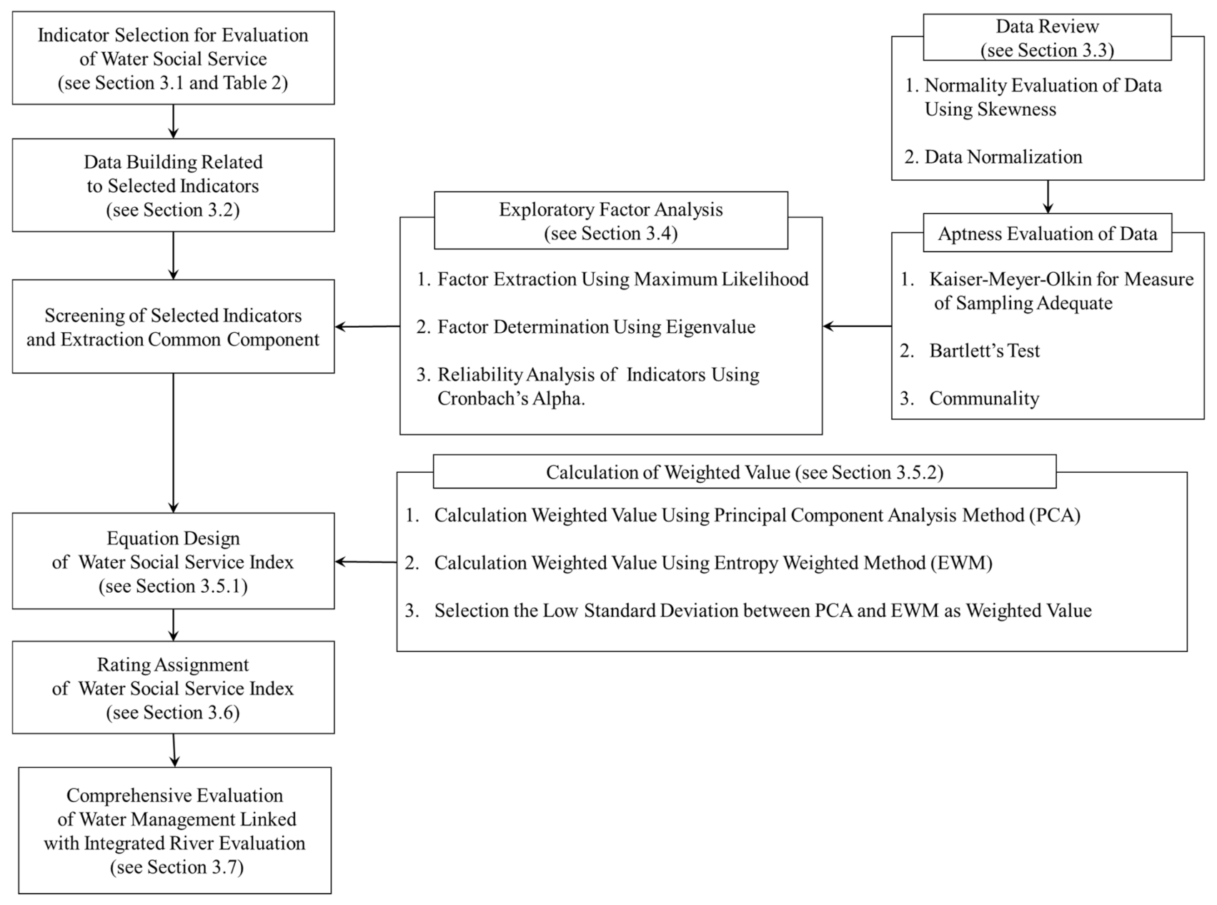
The research methodology is explained in Figure 2. First, the water social service index (WSSI) was selected to evaluate the water social service; relevant indicators were then calculated. The final indicators were selected after examining the adequacy of each indicator, and the equation for calculating the WSSI was developed. Here, to avoid the indicator factors influence each other, a weighted value was calculated and reflected in the WSSI equation. Subsequently, the ratings of water social services were divided into five categories using the indices deduced previously. Finally, the comprehensive evaluation of water management was performed by linking integrated river evaluation ratings and WSSI ratings. The detailed research procedures are further described in Section 3.1, Section 3.2, Section 3.3, Section 3.4, Section 3.5, Section 3.6 and Section 3.7; all the statistical analyses were performed using IBM SPSS Statistics 22 (New York, NY, USA).

3.1. Indicator Selection for Water Social Service Evaluation

In this study, the 15 indicators for four water social service categories shown in

Table 2. Reasons for selection of water social service indicators.

Category	Indicators	Reason for Selection	Abbreviation
Water Supply Capacity	Revenue water ratio	Ratio of revenue water to total water quantity; it represents the transfer efficiency of water delivery/distribution or the actual supply ratio of water	RWR
	Water supply amount	Amount of water supplied for each purpose or the total amount of supplied water; represented as the sum of industrial water and domestic water	WSA
	Water supply and demand ratio	Ratio of supply to demand of water, which identifies the regions having limitations in using water; it compares the usage amount to the available amount of supply	WSDR
Water Usage	Daily water usage per person	Domestic water usage with respect to the population in the watershed; a high indicator value implies the overconsumption of domestic water	DWUP
	Amount of replacement water	Represents the amount of potential water resources, which can replace rivers through recirculation of sewage and reclaimed water	ARW
	Supply ratio of water system	Ratio of the population supplied with water to the entire population; a high indicator value implies that water usage is adequate	SUWS
	Supply ratio of sewer treatment system	Ratio of the population receiving sewage service to the entire population; a high indicator value implies that the water usage is adequate	SRST
Water Service Management	Cost recovery rate of water supply	Rate of water charge to the unit cost of water supply production;a high indicator value implies that the water service management is adequate	CRWS
	Cost recovery rate of sewage service	Rate of sewage service charge to the cost of sewage treatment; a high indicator value implies that the water service management is adequate	CRSS
	Self-reliance ratio of water supply	Ratio of annual revenue to annual expenditure (construction + maintenance costs)/water charge; it represents the self-reliance of water supply service	SRWS
	Self-reliance ratio of sewage service	Ratio of annual revenue to annual expenditure (construction + maintenance costs)/water charge; it represents the self-reliance of sewage service	SRSS
Water Service Equity	Water supply and demand ratio of the elderly population	Water supply and demand ratio per elder; it determines the vulnerability of water supply and demand in the elderly population	WREP
	Water usage amount of the elderly population	Daily water usage amount per elder; it determines the vulnerability of water usage in the elderly population	WUEP
	Water supply and demand ratio of the beneficiaries of national basic livelihood	Water supply and demand ratio of the beneficiaries of national basic livelihood; it determines the vulnerability of water supply and demand of the socioeconomically disadvantaged population	WSDB
	Water usage amount of the beneficiaries of national basic livelihood	Daily water usage amount per beneficiary of national basic livelihood; it determines the vulnerability of water usage of socioeconomically disadvantaged population	WUSB

were selected for evaluating the water social service. The water supply capacity category includes the three indicators as revenue water ratio, water supply amount, and water supply and demand ratio, which indicates the efficiency of the water supply capacity from the perspective of the water supplier. Where, “supply” means the distribution from water supply facilities to consumers. Further, “demand” means the required water quantity from predicted data of the national water supply plan. The water usage category consists of four indicators including the daily water usage per person, amount of replacement water, supply ratio of water system, and supply ratio of sewer treatment system. Where “usage” means actual use from the water consumer. These indicators imply the quantity and a variety of water usage being used from the user’s perspective. The water service management category consists of the cost recovery rate of water supply and sewage as well as the self-reliance ratio of water supply and sewage as detailed indicators, which imply the management level of water services. Lastly, the water service equity category consists of the water supply and demand ratio and water usage amount of the elderly population as well as the beneficiaries of the national basic livelihood, through which the difference in the usage of water service according to socioeconomic characteristics is examined from the perspective of water justice.

3.2. Building Indicator’s Data

The 15 indicators in the four categories for evaluating water social service can be calculated as follows.

(1) Calculating the indicators of water supply capacity category

As earlier mentioned, water supply capacity category includes RWR (%), WSA (ton/year), and WSDR (%). The data for WSA were taken from WAMIS [30], whereas the RWR and WSDR were calculated using Equations (1) and (2).

Here, water demand amount (WDA, ton/year) is the product of population and water supply amount per person (WSAP, ton/year), whereas the WSA (ton/year) is the sum of regional water treatment plant capacity (ton/year) and planned distribution of multi-regional water supply (ton/year).

RWR (%) = DWUP/DWAP

(1)

WSDR (%) = WDA/(WSAP × RWR)

(2)

(2) Calculating the indicators of water usage category

Water usage category includes DWUP (ton/year), ARW (ton/year), SUWS (%), and SRST (%). Raw data were used for DWUP, SEWS, and SRST; however, ARW was calculated using Equation (3). Here, the data of amount of sewage reused (ASR) and reclaimed water usage amount (RWSA) were taken from WAMIS [30].

ARW (ton/year) = ASR (ton/year) + RWAS (ton/year)

(3)

(3) Calculating the indicators of water service management category

Water service management category includes CRWS (%), CRSS (%), SRWS, and SRSS. The data from WAMIS [28] were used for CRWS and CRSS, whereas the SRWS and SRSS, which signify the independence of each service, were calculated using Equations (4) and (5), respectively.

SRWS (non-dimension) = (construction costs + maintenance costs)/water charge

(4)

SRSS (non-dimension) = (construction costs + maintenance costs)/sewage charge

(5)

(4) Calculating the indicators of water service equity category

Water service equity category includes WREP (%), WUEP (ton/year), WSDB (%), and WUSB (ton/year) in which each index was calculated using Equations (6)–(9). In Equations (6)–(9), water demand of the elderly population (WDEP ton/year) and water demand of the beneficiaries of national basic livelihood (WDBP, ton/year) is the product of the relevant population and the water supply amount per person. The amount of water supply to the elderly population (AWEP) and the amount of water supply to the beneficiaries of national basic livelihood (AWBP) was calculated as a ratio of the relevant population to the sum of regional water treatment plant capacity and planned distribution of multi-regional water supply, respectively. Furthermore, the data of daily water usage per elder (DWUE), daily water supply amount per elder (DWAE), daily water usage per beneficiary of national basic livelihood (DWUB), and water supply amount per beneficiary of national basic livelihood (DWAB) were taken from WAMIS [30].

WREP (%) = DWUE/DWAE

(6)

WUEP (%) = WDEP/(AWEP × WREP)

(7)

WSDB (%) = DWUB/DWAB

(8)

WUSB (%) = WDBP/(AWBP × WSDB)

(9)

Here, WDEP and WDBP is the product of the relevant population and the WSA per person. The AWEP and AWBP were calculated as a ratio of the relevant population to the sum of regional water treatment plant capacity and planned distribution of multi-regional water supply, respectively. Here, the regional water treatment plant capacity means the water supply ability of water supply facilities built by a local government. The planned distribution of multi-regional water supply means the data of water supply project planned by a metropolitan government. This data has been offered on the internet.

3.3. Normality and Standardization of Each Indicator’s Data

The raw data are assumed to have a normal distribution for statistical analyses; thus, the range of data has to be matched, or the data distribution needs to be modified to be similar for performing statistical analyses of the collected data. In addition, data must be standardized because different dimensions, scales, or units of the data collected for comparing the results of statistical analyses can generate errors when interpreting the results.

In this study, skewness was used to examine the normality and bias of the indices collected or calculated for each detailed indicator in Section 3.2. In this study, if the skewness of each detailed indicator was between −1 and 1, it was considered that there was no bias. If the skewness was below −1 or greater than 1, the normality was secured by converting with the common log and the natural log, respectively. Then, the standardization was performed to match the scale of the data.

For the standardization of data, a difference from the baseline, scale readjustment, Z-Score, categorical scale, percentage of annual difference over consecutive years, or cycle index can be used [31]. Considering the characteristics of this study, all index values must have the same directionality; however, inverse property of certain data can lead to errors in data interpretation. Thus, the methods mentioned above are not appropriate for standardization in this study. As an alternative, the minimum-to-maximum standardization method that can match the directionality is proposed in which the interpretation error, because of an inverse attribute of the data, can be prevented. Accordingly, the minimum-to-maximum standardization method was adopted in this study, as shown in Figure 3, to standardize the index of each detailed indicator.

3.4. Indicator Selection and Reliability Review

The validity of a measurement tool must be verified because a valid and reliable measurement tool is an essential component of any study, and the interpretation of the findings depends on the validity of the measurement tool [32]. This study tried to use the previous study results to review the construct validity of whether 15 indicators are suitable as tools for evaluating water social services. However, few studies have been conducted in Korea to evaluate water social services, and no basic structure of data has been established for water social service evaluation. Therefore, this study was intended to determine the construct validity by conducting a factor analysis and remove indicators that cannot be interpreted or have low reliability. In general, factor analysis is divided into two categories: Exploratory Factor Analysis (EFA) and Confirmatory Factor Analysis (CFA), depending on the purpose. EFA is used by researchers when there is no definite information about any factors and number of factors, or when the underlying structure of the data is unknown, and CFA is used to hypothesize existing relationships between variables and demonstrate their relationship through factor analysis.

As mentioned earlier, this study judged that EFA is an appropriate method to review the construct validity for selected indicators, as it is difficult to find studies of water social service evaluation in South Korea. Principal Component Analysis (PCA) and Maximum Likelihood (ML) could be suggested as the EFA’s factoring method. PCA and ML are both methods of summarizing or dimension reducing for multiple variables; however, factoring using PCA could lead to false results of larger factor loadings [33]. ML is introduced as a reasonable method to extract common factors under the assumption of the multivariate normal distribution as a method used when the normality of the variables is mostly satisfied [34]. For this reason, this study performed ML used as the factoring method of the EFA to review the construct validity of indicators.

Before conducting the EFA, the data’s adequacy has to be measured. To this end, this study had reviewed the Kaiser–Meyer–Olkin (KMO) and Bartlett’s test, and communality. In general, it is considered appropriate to conduct EFA when the KMO value is greater than 0.5, Bartlett’s test has p (probability) less than 0.1, and communality is 0.5 or greater [35,36,37,38]. Further, the number of components was determined by extracting only the components with an eigenvalue greater than one by Keiser–Guttman method [39,40].

Factor rotation methods for factoring can be suggested with orthogonal rotation and oblique rotation, which ML typically was used the direct Oblimin method, one of the oblique rotation methods. In this study, the direct Oblimin method was used as a factor rotation method. Thus, this paper has reviewed the reliability of extracted indicators using Cronbach’s alpha. Cronbach’s alpha was used to review the internal consistency of indicators. Generally, confidence for application research is obtained when Cronbach’s alpha is more significant than 0.8 [41].

3.5. Index Equation Design and Weighted Value Calculation for Evaluating Water Social Service

3.5.1. Index Equation Design for Evaluating Water Social Service

This study proposed an additive function with the simplest form to calculate the WSSI using the indicator mentioned above’s value. The result of using an additive function has the risk of overestimating when the value of each item is summed. To resolve this issue, an appropriate weighted value could be applied to each indicator; the additive function applied with a weighted value can be represented as shown in Equation (10), in which the sum of weights is one.

$$\mathrm{I} = {\displaystyle \sum }_{\mathrm{i}=1}^{\mathrm{n}}{\mathrm{W}}_{\mathrm{i}}·{\mathrm{I}}_{\mathrm{i}}$$

(10)

Here, W_i denotes the weighted value of each indicator, and I_i presents a standardized indicator value of each category.

3.5.2. Calculating the Weighted Value

Both, the ML and entropy weighted method (EWM), were performed for each indicator in this study to ensure that the weighted value does not allow the indicator factors to influence each other. It should be noted that there could be a compensatory issue owing to the cancellation effect of a low indicator value being diluted by a high indicator value. To prevent such an issue, this study was used a geometric mean to accumulate the indices. The weighted value with the smallest standard deviation was selected among all the values derived through the ML and EWM for calculating the WSSI and ensure that all indicators have an even influence on the outcomes.

Calculation of Weighted Value Using Principal Component Analysis Method

Factor analysis could be described as a technique for defining potential factor structures that describe the correlation structure between variables. The primary purpose of a factor analysis is to explore and identify the latent variables underlying the relationship between variables, i.e., the structure of the factors. This study had intended to calculate the weighted value using the characteristics of factor analysis. To this end, this study adopted the principal components analysis (PCA) method, which was reported by Hotelling [42]. This method, along with Factor analysis, is widely used to analyze qualitative indicators in the social and economic field [43,44,45].

The method of calculating weighted value using PCA method requires component matrix and eigenvalue, which in this study used the structure matrix and eigenvalues derived by ML for them. This study judged that the “structure matrix” is suitable for weighted value calculation because this matrix has elements which are a correlation coefficient that refers to the relationship between factors and variables.

The calculating weighted value using PCA method can be described as follows. When a matrix of k explanatory variables and n observed value is X, the linear combination Z can be expressed as follows: where A is an arbitrary symmetric matrix.

$${\mathrm{Z}}_{\mathrm{ij}} ={ \mathrm{X}}_{\mathrm{ij}}{\mathrm{A}}_{\mathrm{ij}} (\mathrm{i}=1,2, \dots ,\mathrm{k}, \mathrm{j}=1,2,\dots ,\mathrm{n})$$

(11)

Considering the first linear combination, it can be expressed as follows:

$${\mathrm{Z}}_{1\left(\mathrm{n}\times 1\right)} ={ \mathrm{X}}_{1\left(\mathrm{n}\times \mathrm{k}\right)}{\mathrm{A}}_{1\left(\mathrm{k}\times 1\right)}$$

(12)

$${{\mathrm{Z}}^{\prime }}_1{\mathrm{Z}}_1 ={\mathrm{A}{}^{\prime }}_1{\mathrm{X}{}^{\prime } \mathrm{X} \mathrm{A}}_1$$

(13)

Here, when Lagrangian is applied to obtain the largest eigenvalue, it is shown below.

$${\mathrm{Z}{}^{\prime }}_1{ \mathrm{Z}}_1={\mathsf{\lambda }}_1{ \mathrm{A}{}^{\prime }}_1{ \mathrm{A}}_1={\mathsf{\lambda }}_1$$

(14)

If the first eigenvalue is ${\mathsf{\lambda }}_1$, ${\mathsf{\lambda }}_1$ will have the largest eigenvalue of $\left(\mathrm{X}{}^{\prime } \mathrm{X}\right)$. The weighted value can be expressed as follows:

$$\mathrm{Z}{}^{\prime } \mathrm{Z} = \mathrm{A}{}^{\prime } \mathrm{X}{}^{\prime } \mathrm{X} \mathrm{A} = \mathsf{\Lambda } =\left[\begin{array}{ccc}{\mathsf{\lambda }}_1& \cdots & 0\\ ⋮& \ddots & ⋮\\ 0& \cdots & {\mathsf{\lambda }}_{\mathrm{k}}\end{array}\right]\left({ \mathrm{Z}{}^{\prime }}_{\mathrm{i}}{\mathrm{Z}}_{\mathrm{i}}={\mathsf{\lambda }}_{\mathrm{i}} , \mathrm{i}=1,2, \dots \mathrm{k} \right)$$

(15)

Therefore, when ${\mathsf{\lambda }}_1$ is identified, the weighted value can be calculated. Meanwhile, the size of ${\mathrm{X}}_{\mathrm{ij}}$ is determined by $\frac{{\mathsf{\lambda }}_1}{\sum {\mathsf{\lambda }}_{\mathrm{i}}} , \frac{{\mathsf{\lambda }}_2}{\sum {\mathsf{\lambda }}_{\mathrm{i}}} , \dots , \frac{{\mathsf{\lambda }}_{\mathrm{k}}}{\sum {\mathsf{\lambda }}_{\mathrm{i}}}$.

Calculation of Weighted Value Using Entropy Weighted Methods

The entropy weighted methods (EWM) [38] is a method for determining the weighted value of each attribute. The method involves applying simple information theories to decision-making problems having a great number of attributes and alternatives. This particular method can be used for selecting the weighted value based on the attribute information of the evaluation items and for applying the weighted value in a vulnerability assessment. For calculating the weighted value, the attribute information of each evaluation item is extracted and normalized to calculate the entropy of each attribute information and the weighted value of each evaluation item.

The EWM has the advantage of being objective because the weighted value is calculated by considering the distribution of the secured data. Four basic methods used to measure information based on entropy include maximum entropy, joint entropy, conditional entropy, and trans-information. Maximum entropy is derived from statistical physics research and it is a technique that excludes assumptions about unknown facts and sees only known partial facts as a source of knowledge acquisition. This technique can function as a probability model with a uniform distribution for other values if the predefined constraints are met. Maximum entropy is defined as the entropy amount of the probability $p(x_n)$ distribution of the discrete random variable $\mathrm{X}=\left\{{\mathrm{x}}_{\mathrm{n}}\right\}$. Maximum entropy $\mathrm{H}\left(\mathrm{X}\right)$ refers to the uncertainty or information capacity of $\mathrm{X}$, and limit entropy for hydrological random discrete variables is defined as Equation (11).

$$\mathrm{H}\left(\mathrm{X}\right)= -{\displaystyle \sum }_{\mathrm{n}=1}^{\mathrm{N}}\mathrm{p}\left(\mathrm{x}\right)·\mathrm{lnp}\left(\mathrm{x}\right)$$

(16)

Generally, there is the maximum entropy, if the discrete probability variable $\mathrm{X}$ follows a uniform distribution. Further, having a uniform distribution of the maximum entropy model for unknown facts means that the model has maximum entropy for unknown contents. This is considered to be the same probability for two events when there is no information to clearly distinguish a given event; this means that uncertainty is maximized, resulting in maximum entropy.

For example, if ${\mathrm{y}}_{\mathrm{m}}=\left(\mathrm{m}=1,2,\cdots ,\mathrm{N}\right)$ is related to random ${\mathrm{x}}_{\mathrm{n}}$, $\mathrm{H}\left(\mathrm{X}|\mathrm{Y}\right)$ represents the amount of $\mathrm{X}$ information that cannot be represented by the information in $\mathrm{Y}$ and it is expressed as Equation (12).

$$\mathrm{H}\left(\mathrm{X}|\mathrm{Y}\right)= -{\displaystyle \sum }_{\mathrm{n}=1}^{\mathrm{N}}{\displaystyle \sum }_{\mathrm{m}=1}^{\mathrm{N}}\mathrm{p}\left({\mathrm{x}}_{\mathrm{n}},{\mathrm{y}}_{\mathrm{m}}\right)\mathrm{lnp}({\mathrm{x}}_{\mathrm{n}}|{\mathrm{y}}_{\mathrm{m}})$$

(17)

where the probability of combining $\mathrm{p}\left(\mathrm{x},\mathrm{y}\right):\mathrm{X}=\left\{{\mathrm{x}}_{\mathrm{n}}\right\}$ and $\mathrm{Y}=\left\{{\mathrm{y}}_{\mathrm{m}}\right\}$ is $\mathrm{p}({\mathrm{x}}_{\mathrm{n}}|{\mathrm{y}}_{\mathrm{m}})$, and the conditional probability $\mathrm{H}\left(\mathrm{X}|\mathrm{Y}\right)$ of a given and is the conditional entropy of a given $\mathrm{Y}$ and $\mathrm{X}$, which can be interpreted as a loss of information during the process of information transfer between $\mathrm{X}$ and $\mathrm{Y}$ [46].

The brief calculation process of the weighted value by EMW can be summarized as follows:

Step 1: Constructing the attribute matrix using the data of indicators of each watershed.

$$\mathrm{D}= \left(\begin{array}{ccc}{\mathrm{x}}_{11}& \cdots & {\mathrm{x}}_{1\mathrm{n}}\\ ⋮& \ddots & ⋮\\ {\mathrm{x}}_{\mathrm{m}1}& \cdots & {\mathrm{x}}_{\mathrm{mn}}\end{array}\right)$$

(18)

Step 2: Normalizing the data of indicator.

$${\mathrm{p}}_{\mathrm{ij}}= \frac{{\mathrm{x}}_{\mathrm{ij}}}{{{\displaystyle \sum }}_{\mathrm{i}=1}^{\mathrm{m}}{{\displaystyle \sum }}_{\mathrm{j}=1}^{\mathrm{n}}{\mathrm{x}}_{\mathrm{ij}}} \left(\mathrm{i}= 1, 2, \dots , \mathrm{m}; \mathrm{j}= 1, 2, \dots , \mathrm{n}\right)$$

(19)

Step 3: Calculating the Entropy for each data of indicator.

$${\mathrm{E}}_{\mathrm{j}}= -\mathrm{k}{\displaystyle \sum }_{\mathrm{i}=1}^{\mathrm{m}}{\mathrm{p}}_{\mathrm{ij}}{ \log \mathrm{p}}_{\mathrm{ij}} \left(\mathrm{k}= \frac{1}{\log \mathrm{m}}; \mathrm{j}= 1, 2, \dots , \mathrm{n}\right)$$

(20)

Step4: Calculating weighted value for each indicator.

$${\mathrm{w}}_{\mathrm{j}}= \frac{{\mathrm{d}}_{\mathrm{j}}}{{{\displaystyle \sum }}_{\mathrm{j}=1}^{\mathrm{n}}{\mathrm{d}}_{\mathrm{j}}} \left({\mathrm{d}}_{\mathrm{j}}= 1-{ \mathrm{E}}_{\mathrm{j}} ; \mathrm{j}= 1, 2, \dots , \mathrm{n}\right)$$

(21)

3.6. Assigning Ratings to Water Social Service Index

The rating of WSSI was divided into five sections. The calculated index values were assumed to have a Gaussian distribution in this study, and the ratings were given based on the standard deviation. The rating classification based on the standard deviation was determined as proposed in the study by Hwang et al. [26] in which 1 standard deviation (1 σ) was defined as the highest and the lowest ratings. Further, 16% on both left and right ends were defined as the highest rating of 1 and the lowest rating of 5, respectively. The section corresponding to the remaining 68% was divided as 0.5 standard deviation (0.5 σ), 67.5–84.0% was classified as rating 2, 32.5–67.5% was classified as rating 4, and 16.0–32.5% was classified as rating 5 (

Table 3. Rating section for water social service evaluation.

Rating Section		Rating	Key Processing Function
μ + 1.0 σ	100.0–84.0%	1	Very Good (High)
μ + 0.5 σ	84.0–67.5%	2	Good (Medium High)
-	67.5–32.5%	3	Acceptable (Medium)
μ − 0.5 σ	32.5–16.0%	4	Poor (Medium Low)
μ − 1.0 σ	16.0–0.0%	5	Very Poor (Low)

).

3.7. Comprehensive Evaluation of Water Management Based on Matrix Analysis

Another objective of this study is to perform a comprehensive evaluation of water management linked with evaluation results of water quantity and water quality in addition to evaluating water social service. Accordingly, the matrix method was used for the analysis in which the data are visualized by cross-linking two lists consisting of rows and columns. This method examines the correlation of data using a matrix consisting of two or more dimensions [47].

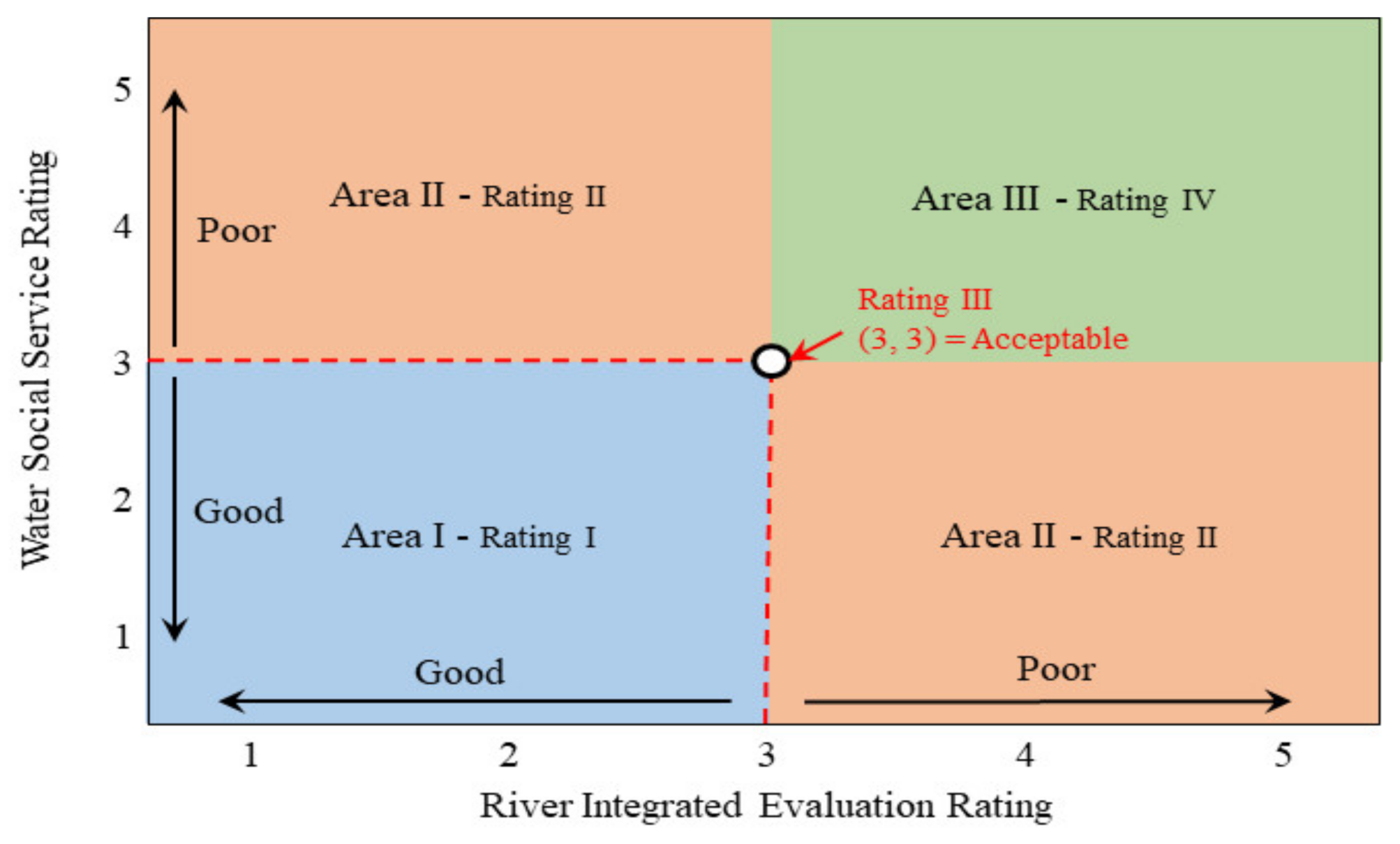
In this study, a comprehensive evaluation of water management was performed using the matrix shown in Figure 4. The x-axis represents the rating of integrated river evaluation, whereas the y-axis represents the rating of water social service. Number 3 on both the x- and y-axis indicates Acceptable or rating 3 of the evaluation items and as the values increase along the x-axis and the y-axis, the rating becomes Poor; and as they decrease, the rating becomes Good. As shown in Figure 4, this matrix is a 2 × 2 matrix that can be divided into 4 sections; however, the matrix is divided into Area I, Area II, and Area III in this study. Area 1 indicates that both integrated river evaluation and water social service evaluations have good ratings where the result of a comprehensive evaluation of water management has a rating I. Two Area IIs indicate that either the integrated river evaluation or the water social service evaluation has a poor rating where the result of a comprehensive evaluation of water management has a rating II. Area III indicates that both integrated river evaluation and water social service evaluations have poor ratings where the result of a comprehensive evaluation of water management has a rating IV. Rating III is either not represented as an area in the matrix, and it is used when the value of both x- and y-axis is 3; it is also the point of intersection in the center in Figure 4. This rating indicates that both integrated river evaluation and water social service evaluations have acceptable ratings where the result of a comprehensive evaluation of water management has a rating III. Thus, the comprehensive evaluation of water management has four ratings where smaller the rating number, better is the rating.

4. Result and Discussion

4.1. Suitability of Collected Data

As the calculation results of 15 indicators’ data by Figure 3 during the study period cannot be fully presented due to the limited space, only the normalization and data conversion results of each detailed indicator’ data are shown in

Table 4. Results of the indicators’ skewness.

Indicator	(a) Skewness before Conversion	(b) Skewness after Conversion
Revenue water ratio (RWR) (%)	1.708	0.226
Water supply amount (WSA) (ton/year)	1.985	−0.008
Water supply and demand ratio (WSDR) (%)	1.161	0.292
Daily water usage per person (DWUP) (ton/year)	1.566	0.483
Amount of replacement water (ARW) (ton/year)	3.586	−0.063
Supply ratio of water system (SUWS) (%)	1.768	0.204
Supply ratio of sewer treatment system (SRST) (%)	1.504	0.313
Cost recovery rate of water supply (CRWS) (%)	1.911	0.137
Cost recovery rate of sewage service (CRSS) (%)	2.536	−0.302
Self-reliance ratio of water supply (SRWS)	2.670	0.278
Self-reliance ratio of sewage service (SRSS)	3.001	0.243
Water supply and demand ratio of the elderly population (WREP) (%)	1.821	0.262
Water usage amount of the elderly population (WUEP) (ton/year)	1.165	0.300
Water supply and demand ratio of the beneficiaries of national basic livelihood (WSDB)	2.016	0.236
Water usage amount of the beneficiaries of national basic livelihood (WUSB)	1.163	0.302

. As mentioned in Section 3.3, skewness was analyzed to review the normality of each detailed indicator’ data, and the results are shown in Table 4 ((a) Skewness before Conversion). The skewness of all detailed indicators’ data is greater than 1 in Table 4 ((a) Skewness before Conversion), thus implying that the data is biased. To resolve this issue, the skewness of each detailed indicators’ data was converted using a natural log to produce the results presented in Table 4 ((b) Skewness after Conversion). The results show that the skewness after conversion of all detailed indicators’ data is between −1 and 1, which implies that the bias has been removed and the normality of indicators’ data secured.

4.2. The Result of KMO, Bartlett’s Unit Matrix Test, and Communality

The adequacy of data must be reviewed before EFA performing for extracting common factors. To this end, the KMO, Bartlett’s test and communality for adequacy review of data were conducted, and the results are shown in

Table 5. Results of Kaiser–Meyer–Olkin (KMO), Bartlett’s test and communality values of the indicators.

Contents			Value
KMO Measure			0.879
Bartlett’s test of sphericity		Approx. Chi-squared	7258.480
		p (significance probability)	<0.001
Communality
No.	Indicators (abbreviation)			Extraction	Remark
1	Revenue water ratio (RWR)			0.996	-
2	Water supply amount (WSA)			0.964	-
3	Water supply and demand ratio (WSDR)			0.997	-
4	Daily water usage per person (DWUP)			0.990	-
5	Amount of replacement water (ARW)			0.844	-
6	Supply ratio of water system (SUWS)			0.999	-
7	Supply ratio of sewer treatment system (SRST)			0.994	-
8	Cost recovery rate of water supply (CRWS)			0.996	-
9	Cost recovery rate of sewage service (CRSS)			0.911	-
10	Self-reliance ratio of water supply (SRWS)			0.973	-
11	Self-reliance ratio of sewage service (SRSS)			0.946	-
12	Water supply and demand ratio of the elderly population (WREP)			0.992	-
13	Water usage amount of the elderly population (WUEP)			1.000	Heywood case (Removed)
14	Water supply and demand ratio of the beneficiaries of national basic livelihood (WSDB)			0.986	-
15	Water usage amount of the beneficiaries of national basic livelihood (WUSB)			1.000	Heywood case (Removed)

. The KMO measured the adequacy to be 0.879, and the Bartlett’s test resulted in a p-value less than 0.001. The data are appropriate for EFA when KMO is above 0.5 [48], Bartlett’s test’s probability value is below 0.1. The KMO adequacy measure and Bartlett’s significance probability satisfied the criteria.

The communality ranged between 0.844 and 1.000, however, the communalities of WUEP and WUSB were presented greater than 1.0.

If the communality is greater than 1.0 which is called the Haywood case [49]. When the Heywood case has occurred, the analysis results should not be accepted because the communality results are not good with the number of factors is not appropriate, the number of variables per factor is small, or the common factor model is not appropriate [50,51,52,53]. In this work, the indicators were removed and the suitability of the data was reviewed again.

4.3. Result of Explatory Factor Analysis

Two indicators with Haywood case were removed from the 15 indicators of Table 5, and a factor analysis was conducted again. KMO, Bartlett’s test, and communality for 13 indicators were reviewed, KMO represent at 0.851 and Bartlett’s p-value below 0.001 (

Table 6. Results of KMO, Bartlett’s test and communality values of the indicators except two Heywood case.

Contents			Value
KMO Measure			0.851
Bartlett’s test of sphericity		Approx. Chi-squared	533.132
		p (significance probability)	<0.001
Communality
No.	Indicators (abbreviation)			Extraction
1	Cost recovery rate of water supply (CRWS)			0.993
2	Supply ratio of water system (SUWS)			0.933
3	Revenue water ratio (RWR)			0.990
4	Water supply amount (WSA)			0.951
5	Supply ratio of sewer treatment system (SRST)			0.574
6	Cost recovery rate of sewage service (CRSS)			0.998
7	Amount of replacement water (ARW)			0.985
8	Water supply and demand ratio of the elderly population (WREP)			0.987
9	Water supply and demand ratio of the beneficiaries of national basic livelihood (WSDB)			0.764
10	Self-reliance ratio of water supply (SRWS)			0.871
11	Daily water usage per person (DWUP)			0.736
12	Water supply and demand ratio (WSDR)			0.990
13	Self-reliance ratio of sewage service (SRSS)			0.977

). Further, the communality of all indicators ranged 0.736–0.998. Therefore, this study determined 13 indicators are suitable for factor analysis.

The EFA of this study was employed the maximum likelihood as factoring method and adapted only the factor with an eigenvalue greater than 1.0 by the Kaiser–Guttman method. As the factoring result, the two factors were extracted that eigenvalue of factor 1 and factor 2 presented 10.500 and 1.606, respectively (

Table 7. Result of eigenvalues and total explained variance.

Factor	Initial Eigenvalues			Extraction Sums of Squared Loadings			Rotation Sums of Squared Loadings
	Total	% of Variance	Cumulative %	Total	% of Variance	Cumulative %	Total
1	10.500	80.770	80.770	10.334	79.494	79.494	9.026
2	1.606	12.351	93.121	1.416	10.892	90.386	8.309
3	0.377	2.899	96.020	-	-	-	-
4	0.215	1.655	97.674	-	-	-	-
5	0.172	1.320	98.995	-	-	-	-
6	0.038	0.295	99.290	-	-	-	-
7	0.033	0.256	99.546	-	-	-	-
8	0.027	0.205	99.752	-	-	-	-
9	0.014	0.110	99.861	-		-	-
10	0.008	0.064	99.925	-	-	-	-
11	0.005	0.036	99.962	-	-	-	-
12	0.004	0.032	99.993	-	-	-	-
13	0.001	0.007	100.000	-	-	-	-

). The criterion for explained variance ratio and cumulative variance ratio of each factor must be specified at least what contribution should be to have practical significance. In this regard, Hair et al. [54] suggested that the social science field’s cumulative explanatory variance should usually be 50–60%. The extraction sum of squared loading of two factors was shown to be 90.386% in Table 7; therefore, this study determined these factors have high explanatory power.

The pattern matrix, structure matrix, Cronbach’s alpha and Goodness of fit test for 13 indicators according to the factor analysis were shown in

Table 8. Result of factor analysis.

No.	Indicators (Abbreviation)		Pattern Matrix		Structure Matrix		Cronbach’s Alpha if Item Delete	Cronbach’s Alpha
			Factor 1	Factor 2	Factor 1	Factor 2
1	Cost recovery rate of water supply (CRWS)		0.985	−0.032	0.991	0.671	0.969	0.978
2	Supply ratio of water system (SUWS)		0.936	0.089	0.978	0.767	0.970
3	Revenue water ratio (RWR)		0.862	−0.192	0.968	0.788	0.970
4	Water supply amount (WSA)		0.837	0.058	0.965	0.581	0.972
5	Supply ratio of sewer treatment system (SRST)		0.816	0.260	0.941	0.832	0.972
6	Cost recovery rate of sewage service (CRSS)		0.779	0.303	0.873	0.578	0.977
7	Amount of replacement water (ARW)		0.691	0.403	0.743	0.344	0.978
8	Water supply and demand ratio of the elderly population (WREP)		−0.008	0.993	0.636	0.995	0.969	0.979
9	Water supply and demand ratio of the beneficiaries of national basic livelihood (WSDB)		0.028	0.978	0.610	0.989	0.969
10	Self-reliance ratio of water supply (SRWS)		−0.088	0.910	0.710	0.916	0.970
11	Daily water usage per person (DWUP)		0.230	0.773	0.842	0.909	0.970
12	Water supply and demand ratio (WSDR)		0.450	0.630	0.796	0.896	0.974
13	Self-reliance ratio of sewage service (SRSS)		0.552	0.653	0.478	0.855	0.979
Goodness of fit test		Chi-squared	765.973
		p	<0.001
Total Cronbach’s alpha			0.980

. Pattern matrix and structure matrix can be used for interpreting of factor analysis result [55]. Some previous studies emphasize structural matrix [56,57,58], or others insist that pattern matrix is essential for interpreting factor analysis result. The matrix selection criteria of factor analysis are unclear; however, this study had adopted a pattern matrix used in many prior studies. Furthermore, the indicators selected only elements representing values greater than 0.4 and utilized them for factor analysis. [59,60].

In Table 8, the indicators of the pattern matrix were represented in order of magnitude. WREP, WSDB, SRWS, and DWUP among the pattern matrix’s Factor 1, CRWS, SUWS, RWR, WSA, SRST, and CRSS among the indicators of the pattern matrix’s Factor 2 were shown to be less than 0.4. Furthermore, Chi-squared and p-value of Goodness of fit test were denoted at 765.973 and less than 0.001, respectively. Consequently, this study judged that factor analysis was conducted appropriately.

By comparing Factor 1 and Factor 2, the indicator was classified into two Factors: Factor 1 included seven indicators (CRWS, SUWS, RWR, WSA, SRST, CRSS, and ARW), and Factor 2 included six indicators (WREP, WSDB, SRWS, DWUP, and SRS). Thus, this study had denominated Factor 1 as “Water Infrastructure” and Factor 2 as “Water Safe” based on the characteristics of each Factor.

The Cronbach’s alpha for each indicator was represented to determine the reliability of Factor in Table 8. The Cronbach’s alpha of Factor 1 and Factor 2 appeared at 0.978 and 0.979, respectively. In general, confidence for application research is obtained when Cronbach’s alpha is more significant than 0.8 [41]. As shown in Table 8, all indicators and the overall Cronbach’s alpha appeared higher than 0.8, ensuring reliability without indicators that undermine reliability and maintaining internal consistency.

4.4. Calculation Results of the Weighted Value of Each Indicator

PCA method and EWM method were performed to calculate the weighted value of each indicator; the results were represented in

Table 9. Results of the weighted value for the detailed indicators.

No.	Factors	Indicators	Symbol of Weighted Value	Weighted Value
				Principal Component Analysis Methods	Entropy Weighted Method
1	Water Infrastructure	Cost recovery rate of water supply (CRWS)	W1	0.0879	0.0807
2		Supply ratio of water system (SRWS SUWS)	W2	0.0856	0.0881
3		Revenue water ratio (RWR)	W3	0.0839	0.0859
4		Water supply amount (WSA)	W4	0.0833	0.0908
5		Supply ratio of sewer treatment system (SRST)	W5	0.0792	0.0857
6		Cost recovery rate of sewage service (CRSS)	W6	0.0682	0.0764
7		Amount of replacement water (ARW)	W7	0.0494	0.0701
8	Water Welfare	Water supply and demand ratio of the elderly population (WREP)	W8	0.0886	0.0668
9		Water supply and demand ratio of the beneficiaries of national basic livelihood (WSDB)	W9	0.0875	0.0630
10		Self-reliance ratio of water supply (SRWS)	W10	0.0751	0.0475
11		Daily water usage per person (DWUP)	W11	0.0739	0.0946
12		Water supply and demand ratio (WSDR)	W12	0.0718	0.0922
13		Self-reliance ratio of sewage service (SRSS)	W13	0.0654	0.0564
Sum				1.0000	1.0000
Standard Deviation				0.0113	0.0150

. The weighted value and rank of PCA method showed that the weighted value for WREP was the highest at 0.0886, followed by the CRWS and WSDB at 0.0879 and 0.0875, respectively. Lastly, the indicator with the lowest weighted value, 0.0494, was the ARW. The weighted value and rank of EMW appeared differently from PCA method. DWUP’s weighted value of EMW method was the highest at 0.0922, SRWS’s weighted value was the lowest at 0.0475.

As mentioned in Section 3.5.2, the weighted value with the smaller standard deviation between the PCA method and EWM method was adopted as the weighted value for WSSI estimation. Table 9 shows that the standard deviation of PCA method is 0.0113, whereas that of EWM method is 0.0150; consequently, the weighted value by PCA method was employed as the weighted value for WSSI estimation.

4.5. Water Social Service Index and Water Social Service Evaluation Results per Watershed

4.5.1. Water Social Service Index

Using the method explained in Section 3.5, an additive function was used to calculate WSSI as shown in Equation (12).

$$\mathrm{WSSI} = \mathrm{WI} + \mathrm{WW}$$

(22)

$$\mathrm{WI} \left(\mathrm{Water} \mathrm{Infrastructure}\right) ={\mathrm{W}}_1{\mathrm{I}}_1+{\mathrm{W}}_2{\mathrm{I}}_2+{\mathrm{W}}_3{\mathrm{I}}_3+{\mathrm{W}}_4{\mathrm{I}}_4+{\mathrm{W}}_5{\mathrm{I}}_5+{ \mathrm{W}}_6{\mathrm{I}}_6 +{ \mathrm{W}}_7{\mathrm{I}}_7$$

(23)

$$\mathrm{WW} \left(\mathrm{Water} \mathrm{Welfare}\right) ={ \mathrm{W}}_8{\mathrm{I}}_8+{\mathrm{W}}_9{\mathrm{I}}_9+{ \mathrm{W}}_{10}{\mathrm{I}}_{10} +{ \mathrm{W}}_{11}{\mathrm{I}}_{11}+{\mathrm{W}}_{12}{\mathrm{I}}_{12}+{\mathrm{W}}_{13}{\mathrm{I}}_{13}$$

(24)

Here, WI refers to the water infrastructure (factor 1), WW refers to the water welfare (factor 2). Furthermore, W₁–W₁₃ represent the weighted values of each indicator in Table 9, whereas I₁–I₁₃ represent the standardized indicators of each watershed. The WSSIs were calculated every year for each watershed using these values, and the WSSI ratings were given.

4.5.2. Water Social Service Index per Watershed

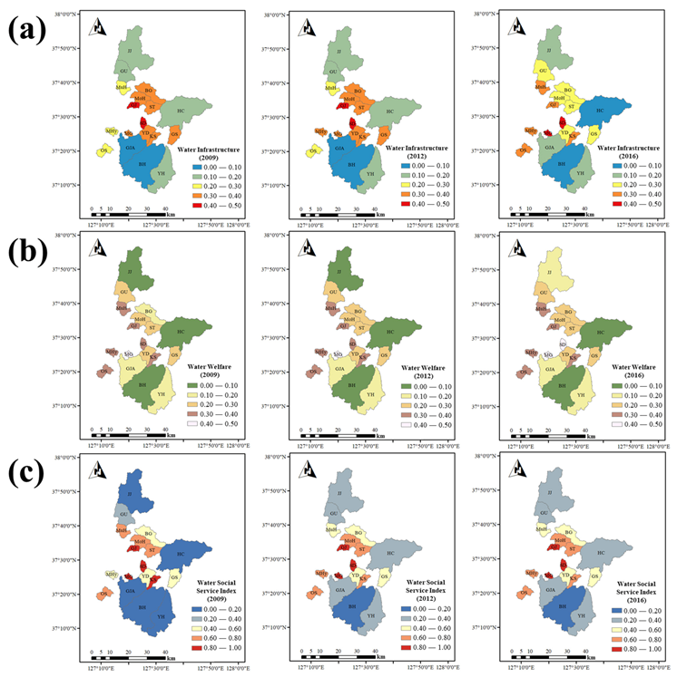
The mean WSSI during the study period is shown in

Table 10. Mean water social service index during the study period.

Study Watershed	Water Infrastructure (WI)		Water Welfare (WW)		Water Social Service Index (WSSI)
	Value	Rank	Value	Rank	Value	Rank
JJ	0.1609	13	0.0922	17	0.2531	14
GU	0.1393	15	0.2375	12	0.3768	13
MuH	0.2374	12	0.3333	7	0.5707	11
BG	0.3078	10	0.2195	13	0.5273	12
MoH	0.3724	6	0.2728	9	0.6452	7
GJ	0.4856	2	0.3790	3	0.8646	2
ST	0.3822	4	0.2821	8	0.6643	6
HC	0.1572	14	0.0713	17	0.2285	16
GS	0.3118	8	0.2592	11	0.5710	10
SD	0.4944	1	0.3872	2	0.8816	1
YD	0.3092	9	0.2653	10	0.5745	9
KS	0.3749	5	0.3391	6	0.7160	4
BH	0.0266	18	0.1761	14	0.1027	18
YH	0.1155	16	0.1223	16	0.2378	15
OS	0.2574	11	0.3556	5	0.6130	8
MHy	0.3142	7	0.3569	4	0.6711	5
GJA	0.0852	17	0.1385	15	0.2237	17
MG	0.4008	3	0.4341	1	0.8349	3
Average	0.2740	–	0.2623	–	0.5309	–
Median	0.3085	–	0.2691	–	0.5728	–

. The average of mean water infrastructure, water welfare and WSSI for all study areas appeared at 0.2740, 0.2623, and 0.5309, respectively. The median of mean water infrastructure, water welfare, and WSSI for all study areas appeared at 0.3085, 0.2691, and 0.5728, respectively. For the water infrastructure indicator, SD (0.4944), GJ (0.4856), and MG (0.4008) had the highest index values in that order; for the water welfare indicator, MG (0.4341), SD (0.3872), and GJ (0.3790) had the highest index values in that order. For WSSI, SD (0.8816), GJ (0.8646), and MG (0.8349) had the highest index values in that order.

Figure 5 shows that the two indicators of water social service are higher when the area of the watershed is smaller, which could be attributed to the high efficiency of water-related infrastructure. In contrast, the index values are lower when the area of the watershed is larger, which indicates the low efficiency of water-related infrastructure.

The study area where Paldang Lake is located is the tough sanction area. Although the study area is the metropolitan area of Korea, the Korean central government has applied very strong regulations to the study area because the Lake Paldang is a very important water resource. For this reason, the population density of study area is very low compared to other metropolitan areas, and local residents live in a large area with the low population density. Due to these characteristics of the study area, the Korean government has been also installing water-related infrastructure, however, in large areas, infrastructure efficiency is inevitably lower than in narrow areas. Although no direct numerical evidence is suggested in this study, the results of this study are relevant considering infrastructure efficiency, which is one of the general characteristics, because the efficiency of infrastructure might be low in regions with strict regulations and slow development, such as a case of this study area.

4.6. Evaluation Results of Water Social Service Index Rating

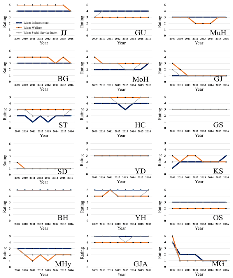
The ratings of water infrastructure, water welfare, and WSSI are presented during the study period in

Table 11. Mean ratings of the water social service during the study period.

Study Watershed	Rating
	Water Infrastructure	Water Welfare	Water Social Service Index
JJ	4	5	4
GU	4	3	4
MuH	3	3	3
BG	3	4	3
MoH	2	3	3
GJ	1	1	1
ST	2	3	2
HC	4	5	5
GS	3	3	3
SD	1	1	1
YD	3	3	3
KS	2	2	2
BH	5	5	5
YH	5	4	5
OS	3	2	3
MHy	3	2	2
GJA	5	4	5
MG	2	2	1

and Figure 6. GJ and SD watersheds had a rating of 1 for water infrastructure and water welfare, which is considered very good, whereas BH, YH, and GJA had a rating of 5 for water infrastructure, and JJ, HC, and BH had a rating of 5, which is considered very poor.

As shown in Table 11, the mean ratings of all the indicators for each watershed are similar without being biased. For example, all the mean ratings of GJ and SD, which were given rating of 1 for WSSI, are either 1, whereas all the mean ratings of HC, BH, YH, and GJA, which were given rating of five for WSSI, are either four or five. Specifically, it indicates that there is a substantial gap in the WSSI between the different watersheds. As the mean ratings are similar for all the WSSI, the watersheds with poor WSSI need improvements in all the sectors rather than in a specific sector.

Figure 6 shows the changes in the annual rating of water infrastructure, water welfare, and WSSI. Most of the WSSI did not vary significantly except MG watershed. These results may correspond to the efficiency of water-related infrastructure mentioned previously in Section 4.5.2. However, the lack of change in WSSI over a long period also signifies a lack of awareness of water social service in each watershed. In particular, we have attributed this result to the indifference to the underprivileged of local government who are responsible for the installation and operation of water-related infrastructure. Another reason for the lack of change in the WSSI is low community awareness among the local residents. From the perspective of human right on water or water justice, a prolonged low WSSI signifies that the elderly population or the beneficiaries of national basic livelihood have been experiencing discrimination or limitations of water usage for the duration study period or longer. Particularly, the WSSI of JJ, GJA, and HC watersheds have remained at 4 or 5, which indicates that the residents in these respective regions have not been receiving universal welfare benefits in terms of water-related services for an extended period.

Accordingly, the water management evaluation based on the WSSI from the perspective of human right to water and water justice enables the status of universal water welfare to be assessed objectively, contrary to the vague expectations that all the users have access to the supplied water without any difficulty. Therefore, the results can be utilized as the basic materials for setting the future direction of advanced water management. Moreover, plans can be established for each sector depending on the results of water social service indicators, and thus a more efficient water management can be gradually designed.

4.7. Result of Comprehensive Evaluation of Water Management Based on Matrix Analysis

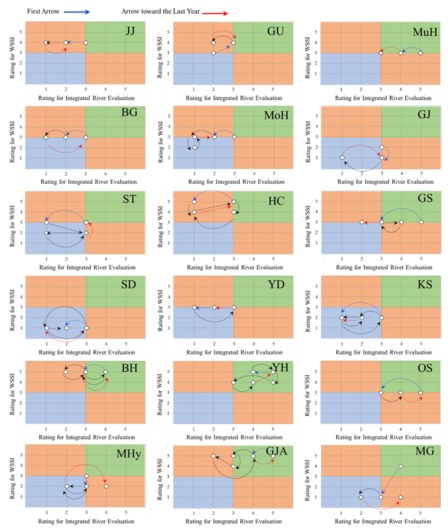
Figure 7 shows the results of a comprehensive evaluation of water management of the study area based on a matrix analysis. The x-axis represents the rating of the integrated river evaluation, whereas the y-axis represents the rating of water social service. As previously mentioned in Section 2.2, the findings of the study by Hwang et al. [26] were used as the data for representing the x-axis.

The results of comprehensive evaluation of water management are depicted as blue, black, and red arrows to represent the changes over time. The blue arrow represents the first movement, black arrow represents the following movement, and red arrow represents the last movement. As shown in Figure 7, results of the comprehensive evaluation of water management move horizontally with the flow of time. It can be inferred that most WSSI ratings are constant over time, such as Figure 6, and the horizontal movement is because of the changes in the ratings of integrated river evaluation. When the changes in the ratings of a comprehensive evaluation of water management are examined, there is no abrupt change in the comprehensive evaluation of water management of each watershed. In particular, the rating moved to an adjacent area of the 2 × 2 matrix or stayed within the area where the first comprehensive evaluation of water management result was given. Especially, in the 11 watersheds including GU, BG, ST, HC, YD, BH, YH, OS, MHy, GJA, and MG among the total 18 watersheds in this study, the water management level did not improve over time and reverted to the original rating.

Furthermore, the WSSI of MG was one; however, their final integrated river evaluation rating was 3 or 4, which resulted in the comprehensive evaluation rating of water management to be rating II. The three watersheds BH, YH, and GJA have a poor rating for both the integrated river evaluation and the water social service thus having the comprehensive evaluation rating of water management placed in Rating IV. Hence, even if a watershed has a good water social service rating, the comprehensive evaluation of water management may be low owing to the poor rating of the integrated river evaluation. The watershed with a poor water social service rating also has a poor integrated river evaluation rating, thus having a low comprehensive evaluation rating of water management.

The comprehensive evaluation of water management using a matrix enables comprehensive monitoring of water management status of each watershed, and thus is an evaluation tool or a minimum indicator for water management of watersheds. The comprehensive evaluation of water management by matrix analysis enables the vulnerabilities in water management to be identified intuitively, unlike the other evaluation systems that are biased or concentrated on one side, thus allowing the policy makers or administrators of water-related matters to recognize the changes in water management status over a period. Moreover, the direction of complex water management can be set by visually representing the susceptible aspects of water management. The regular inspection results can be easily presented in a matrix, thus facilitating an immediate decision-making process.

However, the comprehensive evaluation of water management by matrix analysis only uses two axes; therefore, it has a limitation of using two criteria for evaluating the status of complex water management.

5. Conclusions

This study proposes a method to evaluate water social service. The water social service of each watershed in the study area was evaluated, and the vulnerable aspects in terms of the human right to water and water justice were identified. Moreover, the status of water social service over a period could be examined to address the low awareness of water welfare among the local governments and residents. In addition, a method of comprehensive evaluation of water management using a matrix analysis was proposed through which comprehensive monitoring of water management is possible. However, if some country has no source data or difficulty of using data, it might be challenging to produce results such as this study. This case could be explained as the limitations of this study though it is not only the fields considered in this study intended to judge water management comprehensively. Nevertheless, if the methodology proposed in this study is used using data that could be used depending on the circumstances or conditions, this paper believes that comprehensive water management evaluation of the watershed (or countries) will be possible.

The methodology proposed in this study has certain limitations, such as employing only two axes in matrix analysis; however, it can be expected to prevent discriminations in water usage against the disadvantaged group by evaluating the water social service to promote a society in which universal water welfare is secured. The comprehensive evaluation of water management using a matrix can help decision makers or administrators to recognize the changes in water management status over a period, and thus lead to efficient water management. Furthermore, the proposed methodology can promote the establishment of a systematic and comprehensive water management system at a national level, while being utilized as an alternative for water management in regions having a similar topology as South Korea.

References

1. Sullivan, C.A.; Huntingford, C. Water Resources, Climate Change and Human Vulnerability. In Proceedings of the 18th World IMACS/MODSIM Congress, Cairns, Australia, 13–17 July 2009; Available online: www.mssanz.org.au/modsim09 (accessed on 20 September 2020).
2. World Health Organization; Unicef. Progress on Drinking Water, Sanitation and Hygiene: 2017 Update and SDG Baselines; World Health Organization: Geneva, Switzerland, 2017; p. 24. Available online: apps.who.int/iris/bitstream/handle/10665/258617/9789241512893-eng.pdf (accessed on 21 October 2020).
3. Birol, F. World Energy Outlook; International Energy Agency: Paris, France, 2008; Volume 23, p. 329. Available online: vnk.fi/documents/10616/339615/TN-esitykset_14-04-07.pdf/392ed88f-04ed-41d6-a904-58e1eb044f9b/TN-esitykset_14-04-07.pdf (accessed on 10 October 2020).
4. Tularam, G.A.; Krishna, M. Sequences of groundwater pumping in Australia: A review of impacts around the globe. J. ASES 2009, 4, 151–166. [Google Scholar]
5. Biswas, A.K. Integrated Water Resources Management: A Reassessment; Water International: London, UK, 2004; Volume 29, pp. 248–256. Available online: eclass.duth.gr/modules/document/file.php/TMC338/Integrated%20Water%20Resources%20Management%20A%20Reassessment.pdf (accessed on 18 August 2020).
6. Molle, F. River-basin planning and management: The social life of a concept. Geoforum 2009, 40, 484–494. [Google Scholar] [CrossRef]
7. Programme Hydrologique International. IWRM Guidelines at River Basin Level; UNESCO: Paris, France, 2009. [Google Scholar]
8. Amalia, M.S.; Soedjono, E.S. Ensuring water availability in surabaya through integrated water resources. J. Teknik ITS 2019, 8, 102–108. [Google Scholar] [CrossRef]
9. Ellis, K.; Feris, L. The Right to Sanitation: Time to Delink from the Right to Water. Hum. Rights Q. 2014, 36, 607–629. [Google Scholar] [CrossRef]
10. McCaffrey, S.C. A human right to water: Domestic and international implications. Georget. Environ. Law Rev. 1992, 5, 1. [Google Scholar]
11. Anderton, D.L.; Anderson, A.B.; Oakes, J.M.; Fraser, M.R. Environmental equity: The demographics of dumping. Demography 1994, 31, 229–248. [Google Scholar] [CrossRef]
12. Yu, S.; He, L.; Lu, H. An environmental fairness-based optimization model for the decision-support of joint control over the water quantity and quality of a river basin. J. Hydrol. 2016, 535, 366–376. [Google Scholar] [CrossRef]
13. Mohai, P.; Pellow, D.; Timmons Roberts, J. Environmental Justice. Annu. Rev. Environ. Resour. 2009, 34, 405–430. [Google Scholar] [CrossRef]
14. Mohai, P.; Bryant, B. Environmental injustice: Weighing race and class as factors in the distribution of environmental hazards. Univ. Colo. Law Rev. 1992, 63, 921. [Google Scholar]
15. Goff, M.; Crow, B. What is water equity? The unfortunate consequences of a global focus on in the distribute. Water Int. 2014, 39, 159–171. [Google Scholar] [CrossRef]
16. Falkenmark, M.; Lundqvist, J.; Widstrand, C. Macro-scale water scarcity requires micro-scale approaches. Nat. Resour. Forum 1989, 13, 258–267. [Google Scholar] [CrossRef] [PubMed]
17. Engelman, R.; LeRoy, P. Sustaining Water: Population and the Future of Renewable Water Supplies; Population and Environment Program: Washington, DC, USA, 1993. [Google Scholar]
18. Gleick, P.H. Basic water requirements for human activities: Meeting basic needs. Water Int. 1996, 21, 83–92. [Google Scholar] [CrossRef]
19. Sullivan, C. Calculating a water poverty index. World Dev. 2002, 30, 1195–1210. [Google Scholar] [CrossRef]
20. Environmental Protection Agency. Planning for Sustainability: A Handbook for Water and Wastewater Utilities; EPA: Washington, DC, USA, 2012. Available online: www.epa.gov/sites/production/files/2016-01/documents/planning-for-sustainability-a-handbook-for-water-and-wastewater-utilities.pdf (accessed on 11 May 2020).
21. Hoffjan, A.; Federico, V.D.; Liserra, T.; Müller, N.A. Financial Sustainability Rating Tool for Urban Water Systems; TRUST, European Union. 2014. Available online: http://riunet.upv.es/bitstream/handle/10251/35739/D221_final.pdf?sequence=1 (accessed on 29 May 2020).
22. Comber, A.; Brunsdon, C.; Green, E. Using a gis-based network analysis to determine urban greenspace accessibility for different ethnic and religious groups. Landsc. Urban Plan. 2008, 86, 103–114. [Google Scholar] [CrossRef] [Green Version]
23. The Organization for Economic Co-Operation and Development (OECD). Handbook on Constructing Composite Indicators: Methodology and User Guide; OECD Publishing: Paris, France, 2008; Available online: https://www.oecd.org/std/42495745.pdf (accessed on 17 October 2017).
24. Gómez-Limón, J.A.; Sanchez-Fernandez, G. Empirical evaluation of agricultural sustainability using composite indicators. Ecol. Econ. 2010, 69, 1062–1075. [Google Scholar] [CrossRef]
25. Nguefack-Tsague, G.; Klasen, S.; Zucchini, W. On weighting the components of the human development index: A statistical justification. J. Hum. Dev. Capab. 2011, 12, 183–202. [Google Scholar] [CrossRef]
26. Hwang, J.H.; Park, S.H.; Song, C.M. A Study on an Integrated Water Quantity and Water Quality Evaluation Method for the Implementation of Integrated Water Resource Management Policies in the Republic of Korea. Water 2020, 12, 2346. [Google Scholar] [CrossRef]
27. Sullivan, C.A.; Meigh, J.R.; Giacomello, A.M. The Water Poverty Index: Development and Application at the Community Scale. In Natural Resources Forum; Blackwell Publishing Ltd.: Oxford, UK, 2003; Volume 27, pp. 189–199. [Google Scholar]
28. USDA. United States Department of Agriculture, Washington, DC, USA. Available online: www.usda.gov (accessed on 13 June 2011).
29. World Health Organization. International Decade for Action Water for Life, 2005–2015; WHO: Geneva, Switzerland, 2005; Volume 80, pp. 195–200. Available online: apps.who.int/iris/bitstream/handle/10665/232807/WER8022_195-200.PDF (accessed on 21 June 2019).
30. WAMIS: Water Management Information System, National Institute of Environmental Research. Available online: www.water.nier.go.kr (accessed on 1 March 2020).
31. Nardo, M.; Saisana, M.; Saltelli, A.; Tarantila, S.; Hoffman, A.; Giovannini, E. Handbook on Constructing Composite Indicators: Methodology and User Guide; OECD Statistics Working Papers 2005/3; OECD Publishing: Paris, France, 2005. [Google Scholar]
32. Zagheri Tafreshi, M.; Yaghmaei, F. Factor analysis of construct validity: A review of nursing articles. J. Med. Ed. 2006, 10, 19–26. [Google Scholar]
33. Snook, S.C.; Gorsuch, R.L. Component analysis versus common factor analysis: A Monte Carlo study. Psychol. Bull. 1989, 106, 148–154. [Google Scholar] [CrossRef]
34. Worthington, R.L.; Whittaker, T.A. Scale development research: A content analysis and recommendations for best practices. Couns. Psychol. 2006, 34, 806–838. [Google Scholar] [CrossRef]
35. Li, M.; Yang, J.; Li, Y. An Empirical Study on the Effect of Information-Based Teaching of Ideological and Political Courses in Higher Vocational Colleges Based on Moso Teach. In International Conference on E-Learning, E-Education, and Online Training; Springer: Cham, Switzerland, 2019; pp. 417–428. [Google Scholar] [CrossRef]
36. Kaiser, H.F. An index of factorial simplicity. Psychometrika 1974, 39, 31–36. [Google Scholar] [CrossRef]
37. Hutcheson, G.D.; Sofroniou, N. The Multivariate Social Scientist: Introductory Statistics Using Generalized Linear Models; Sage: Thousand Oaks, CA, USA, 1999. [Google Scholar]
38. Shannon, C.E.; Weaver, W. The Mathematical Theory of Communication; The University of Illinois Press: Urbana, IL, USA, 1949. [Google Scholar]
39. Guttman, L. Some necessary conditions for common-factor analysis. Psychometrika 1954, 19, 149–161. [Google Scholar] [CrossRef]
40. Kaiser, H.F. The application of electronic computers to factor analysis. Ed. Psychol. Meas. 1960, 20, 141–151. [Google Scholar] [CrossRef]
41. Nunnally, J.C.; Bernstein, I.H. Psychometric Theory, 3rd ed.; McGraw-Hill.: New York, NY, USA, 1994. [Google Scholar]
42. Hotelling, H. Analysis of a complex of statistical variables into principal components. J. Ed. Psychol. 1936, 24, 417–441. [Google Scholar] [CrossRef]
43. Johnston, J. Econometric Methods, 3rd ed.; McGraw-Hill: New York, NY, USA, 1985. [Google Scholar]
44. Theil, H. Principles of Econometrics; John Wiley & Sons, Inc.: New York, NY, USA, 1971. [Google Scholar]
45. Maddala, G.S. Introduction to Econometrics, 3rd ed.; Wiley & Sons, Inc.: New York, NY, USA, 2001. [Google Scholar]
46. Yang, Y.; Burn, D.H. An entropy approach to data collection network design. J. Hydrol. 1994, 157, 307–324. [Google Scholar] [CrossRef]
47. Miles, M.B.; Huberman, A.M. Qualitative Data Analysis: An Expanded Sourcebook; Sage Publication: London, UK, 1994; pp. 232–239. [Google Scholar]
48. Cerny, C.A.; Kaiser, H.F. A study of measure of sampling adequacy for factor-analytic correlation matrices. Multivar. Behav. Res. 1997, 12, 43–47. [Google Scholar] [CrossRef] [PubMed]
49. Kolenikov, S.; Bollen, K.A. Testing negative error variances: Is a heywood case a symptom of misspecification? Sociol. Methods Res. 2012, 41, 124–167. [Google Scholar] [CrossRef]
50. Fabrigar, L.R.; Wegener, D.T.; MacCallum, R.C.; Strahan, E.J. Evaluating the use of exploratory factor analysis in psychological research. Psychol. Methods 1999, 4, 272–299. [Google Scholar] [CrossRef]
51. Kline, R.B. Principles and Practice of Structural Equation Modeling, 3rd ed.; Guilford Press: New York, NY, USA, 2011. [Google Scholar]
52. Loehlin, J.C. Latent Variable Models, 4th ed.; Lawrence Erlbaum: Mahwah, NJ, USA, 2004. [Google Scholar]
53. McDonald, R.P. Factor Analysis and Related Methods; Lawrence Erlbaum: Hillsdale, NJ, USA, 1985. [Google Scholar]
54. Hair, J.F., Jr.; Anderson, R.E.; Tatham, R.L.; Black, W.C. Multivariate Data Analysis, 4th ed.; Prentice Hall: Upper Saddle River, NJ, USA, 1995. [Google Scholar]
55. Gorsuch, R.L. Factor Analysis, 2nd ed.; Lawrence Erlbaum: Hillsdale, NJ, USA, 1983. [Google Scholar]
56. Harman, H.H. Modern Factor Analysis, 3rd ed.; Chicago University Press: Chicago, IL, USA, 1976. [Google Scholar]
57. Lattin, J.; Carroll, J.D.; Green, P.E. Analyzing Multivariate Data; Cengage Learning: New York, NY, USA, 2002. [Google Scholar]
58. Tabachnick, B.G.; Fidell, L.S. Using Multivariate Statistics, 5th ed.; Allyn & Bacon: Boston, MA, USA, 2007. [Google Scholar]
59. Merenda, P.F. A guide to the proper use of factor analysis in the conduct and reporting of research: Pitfalls to avoid. Meas. Eval. Couns. Dev. 1997, 30, 156–164. [Google Scholar] [CrossRef]
60. Hair, J.F.; Tatham, R.L.; Anderson, R.E.; Black, W. Multivariate Data Analysis, 5th ed.; Prentice Hall Inc.: Upper Saddle River, NJ, USA, 1998. [Google Scholar]
Figure 1. Scheme of study watersheds.
Water 13 00706 g001
Figure 2. Study process of water social service evaluation and water management comprehensive evaluation.
Water 13 00706 g002
Figure 3. Minimum-to-maximum standardization method.
Water 13 00706 g003
Figure 4. Matrix for water management comprehensive evaluation.
Water 13 00706 g004
Figure 5. Spatial variation of the detailed indicators during the study period: (a) Water Infrastructure; (b) Water Welfare; (c) Water Social Service Index.
Water 13 00706 g005
Figure 6. Annual rating variation in the index detailed indicators and WSSI (orange line) during the study period.
Water 13 00706 g006
Figure 7. Results of the water management comprehensive evaluation using matrix analysis during the study period.
Water 13 00706 g007