
Saturated Hydraulic Conductivity Estimation Using Artificial Neural Networks

 ,
,  ,
,  , ,
, ,  and
and
Abstract
:1. Introduction
2. Materials and Methods
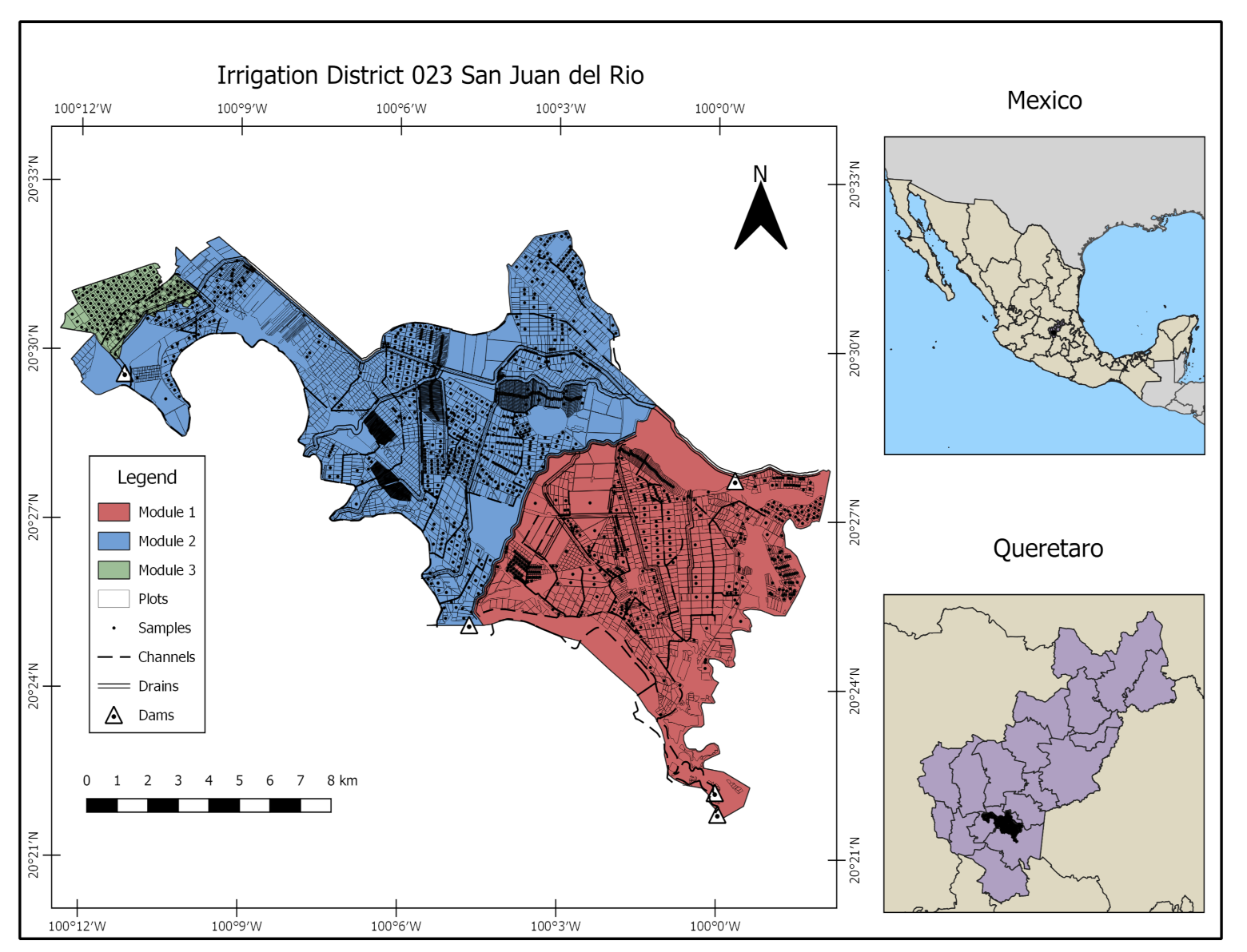
2.1. Study Area
2.2. Soil Database
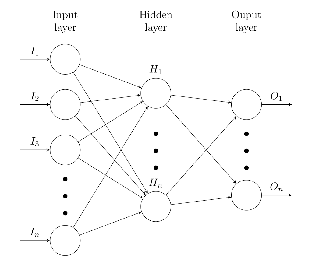
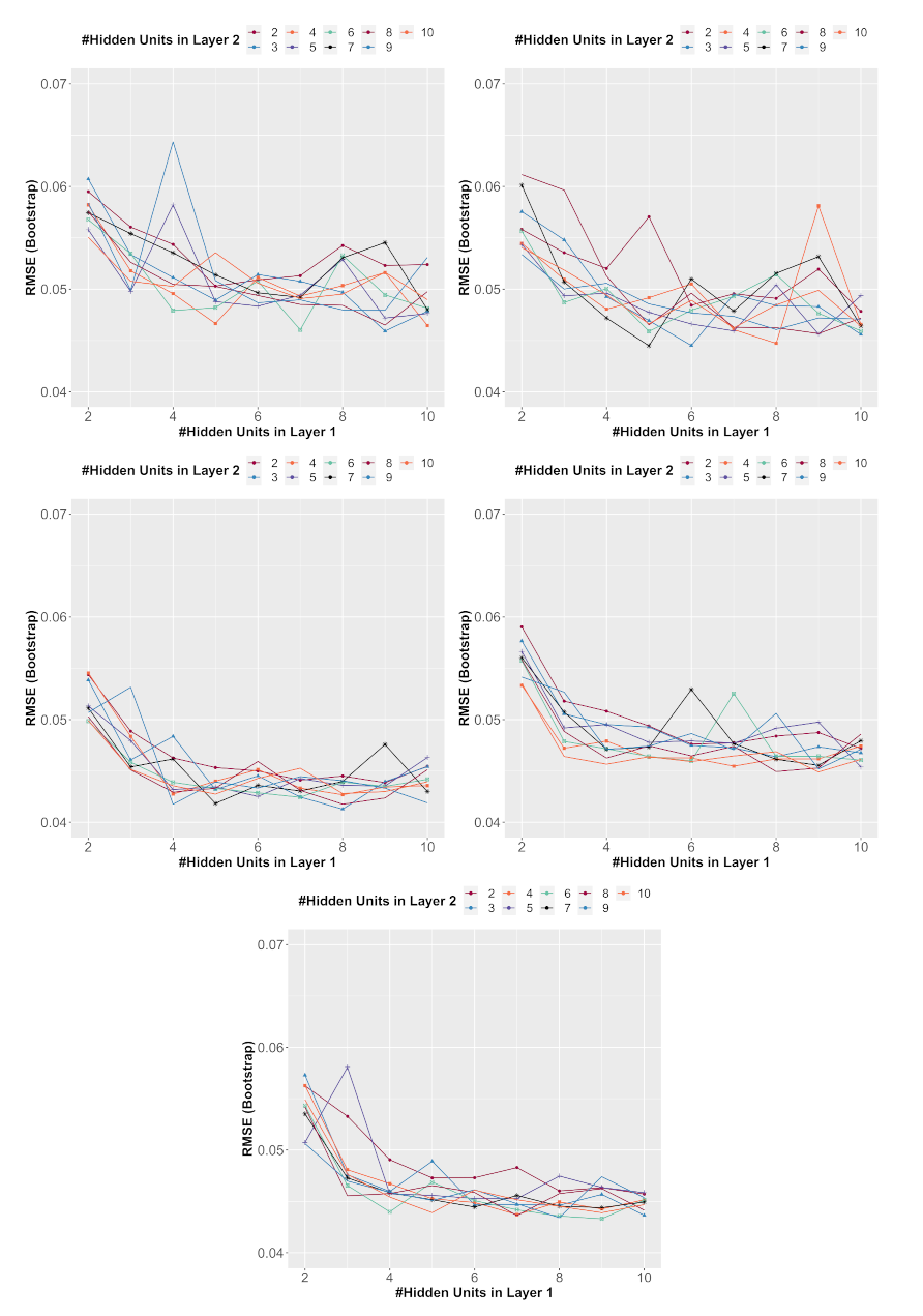
2.3. The ANNs’ Setup
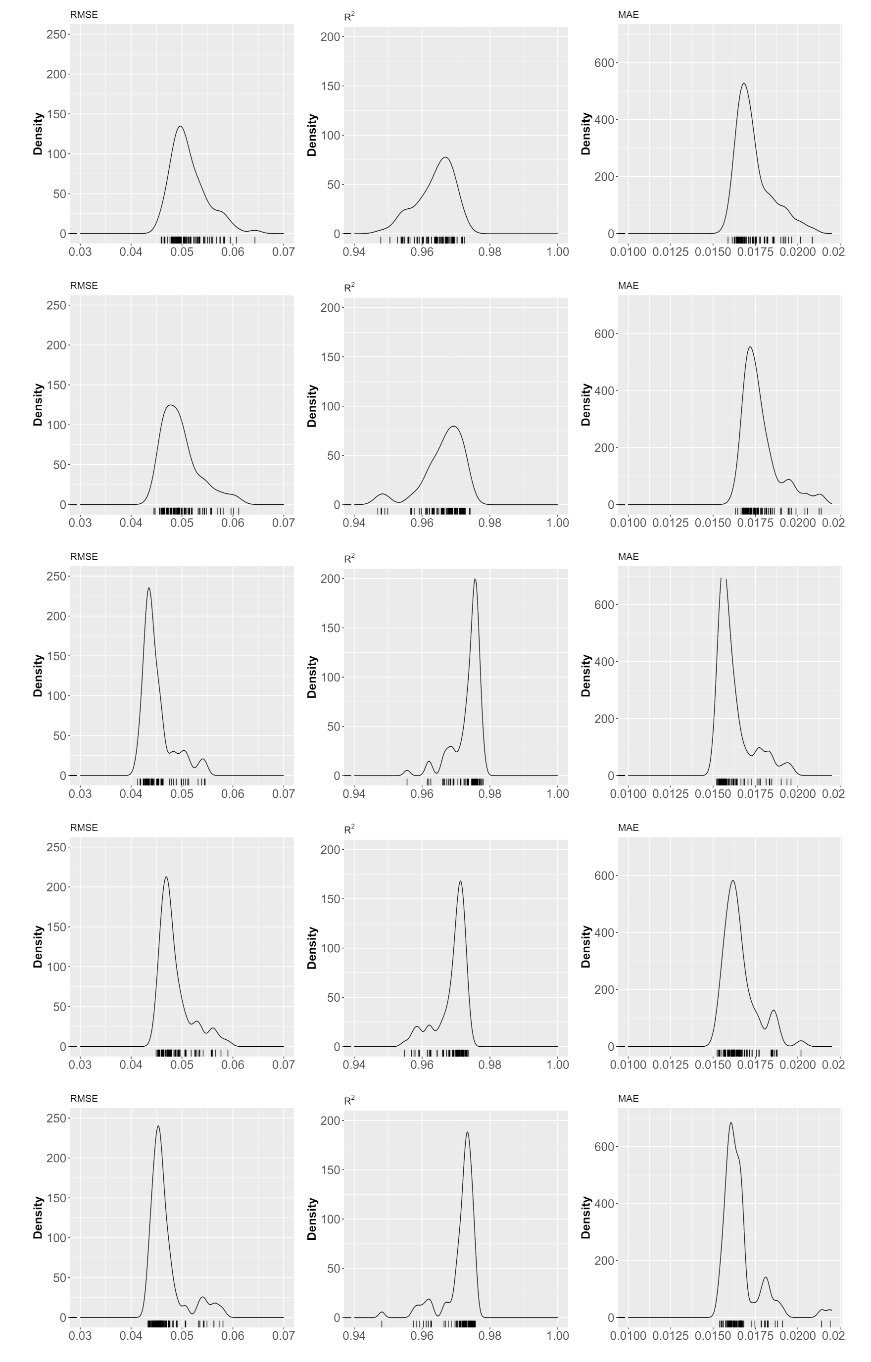
2.4. Cross-Validation
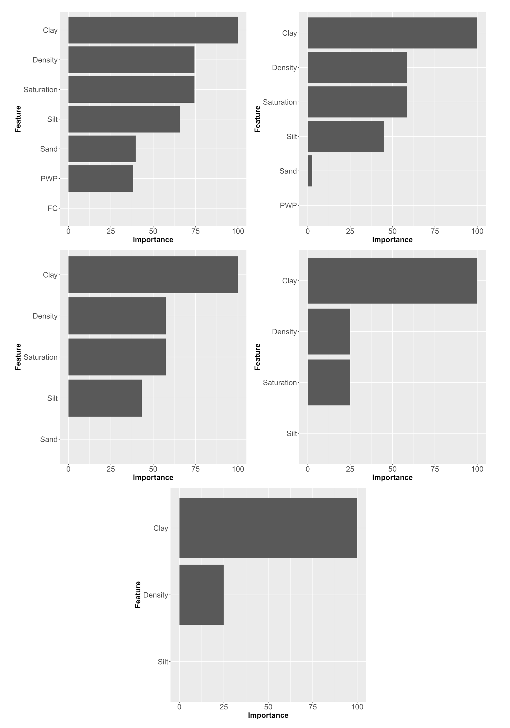
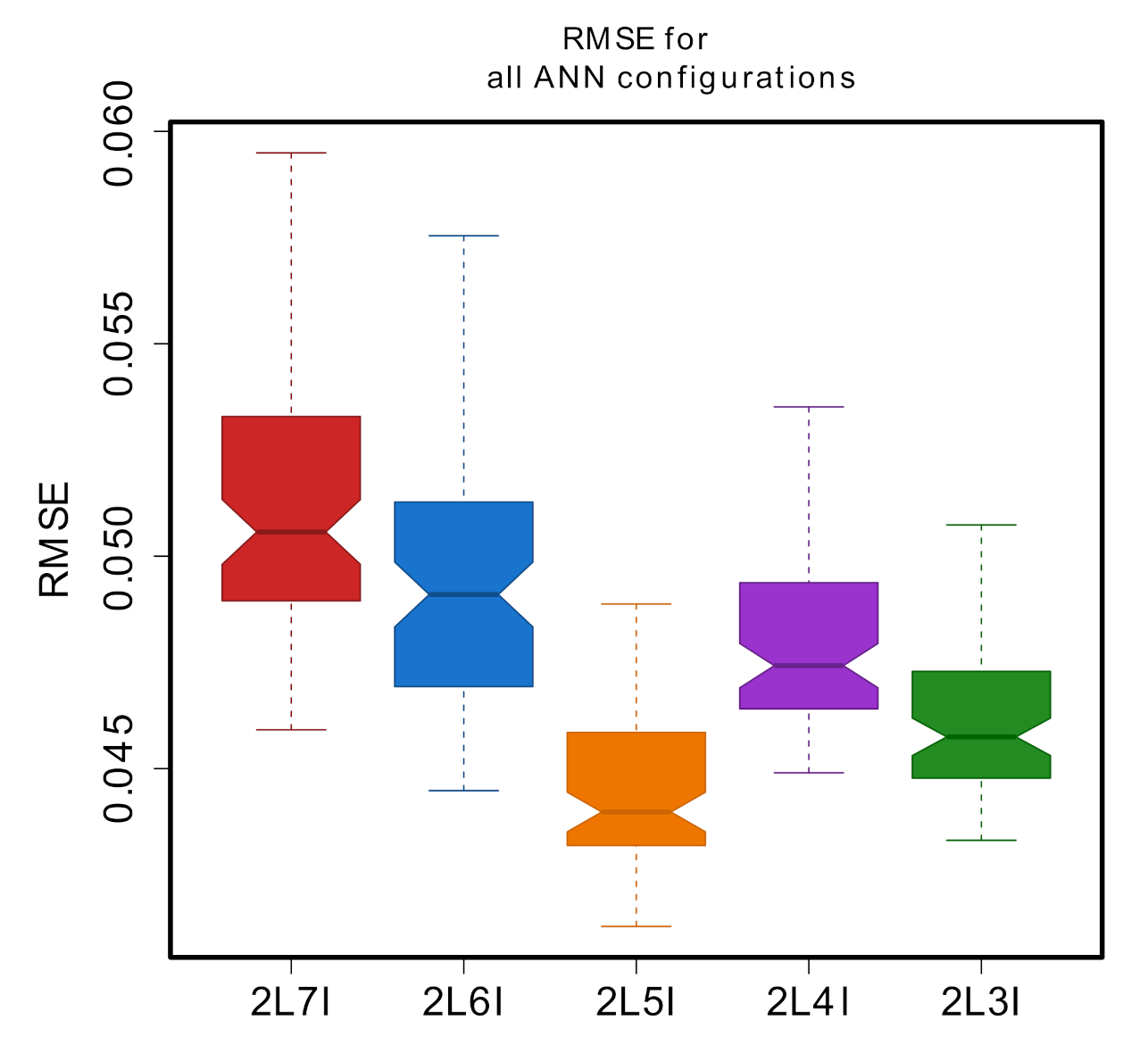
3. Results and Discussion
4. Conclusions
Author Contributions
Funding
Conflicts of Interest
References
- Fuentes, S.; Trejo-Alonso, J.; Quevedo, A.; Fuentes, C.; Chávez, C. Modeling Soil Water Redistribution under Gravity Irrigation with the Richards Equation. Mathematics 2020, 8, 1581. [Google Scholar] [CrossRef]
- Chávez, C.; Fuentes, C. Design and evaluation of surface irrigation systems applying an analytical formula in the irrigation district 085, La Begoña, Mexico. Agric. Water Manag. 2019, 221, 279–285. [Google Scholar] [CrossRef]
- Di, W.; Xue, J.; Bo, X.; Meng, W.; Wu, Y.; Du, T. Simulation of irrigation uniformity and optimization of irrigation technical parameters based on the SIRMOD model under alternate furrow irrigation. Irrig. Drain 2017, 66, 478–491. [Google Scholar]
- Gillies, M.H.; Smith, R.J. SISCO: Surface irrigation simulation, calibration and optimization. Irrig. Sci. 2015, 33, 339–355. [Google Scholar] [CrossRef]
- Saucedo, H.; Zavala, M.; Fuentes, C. Complete hydrodynamic model for border irrigation. Water Technol. Sci. 2011, 2, 23–38. [Google Scholar]
- Weibo, N.; Ma, X.; Fei, L. Evaluation of infiltration models and variability of soil infiltration properties at multiple scales. Irrig. Drain 2017, 66, 589–599. [Google Scholar]
- Zhang, Y.; Schaap, M.G. Estimation of saturated hydraulic conductivity with pedotransfer functions: A review. J. Hydrol. 2019, 575, 1011–1030. [Google Scholar] [CrossRef]
- Abdelbaki, A.M. Evaluation of pedotransfer functions for predicting soil bulk density for U.S. soils. Ain Shams Eng. J. 2018, 9, 1611–1619. [Google Scholar] [CrossRef]
- Brakensiek, D.; Rawls, W.J.; Stephenson, G.R. Modifying SCS Hydrologic Soil Groups and Curve Numbers for Rangeland Soils; Paper No. PNR-84203; ASAE: St. Joseph, MN, USA, 1984. [Google Scholar]
- Rasoulzadeh, A. Estimating Hydraulic Conductivity Using Pedotransfer Functions. In Hydraulic Conductivity-Issues, Determination and Applications; Elango, L., Ed.; InTech: Rijeka, Croatia, 2011; pp. 145–164. [Google Scholar]
- Moreira, L.; Righetto, A.M.; Medeiros, V.M. Soil hydraulics properties estimation by using pedotransfer functions in a northeastern semiarid zone catchment, Brazil. International Environmental Modelling and Software Society, 2004, Osnabrueck. Complexity and Integrated Resources Management. In Transactions of the 2nd Biennial Meeting of the International Environmental Modelling and Software Society, iEMSs 2004; International Environmental Modelling and Software Society: Manno, Switzerland, 2004; Volume 2, pp. 990–995. [Google Scholar]
- Erzin, Y.; Gumaste, S.D.; Gupta, A.K.; Singh, D.N. Artificial neural network (ANN) models for determining hydraulic conductivity of compacted fine-grained soils. Can. Geotech. J. 2009, 46, 955–968. [Google Scholar] [CrossRef]
- Agyare, W.A.; Park, S.J.; Vlek, P.L.G. Artificial Neural Network Estimation of Saturated Hydraulic Conductivity. VZJAAB 2007, 6, 423–431. [Google Scholar] [CrossRef]
- Sonmez, H.; Gokceoglu, C.; Nefeslioglu, H.A.; Kayabasi, A. Estimation of rock modulus: For intact rocks with an artificial neural network and for rock masses with a new empirical equation. Int. J. Rock Mech. Min. Sci. Geomech. Abstr. 2006, 43, 224–235. [Google Scholar] [CrossRef]
- Grima, M.A.; Babuska, R. Fuzzy model for the prediction of unconfined compressive strength of rock samples. Int. J. Rock Mech. Min. Sci. Geomech. Abstr. 1999, 36, 339–349. [Google Scholar] [CrossRef]
- Haque, M.E.; Sudhakar, K.V. ANN back-propagation prediction model for fracture toughness in microalloy steel. Int. J. Fatigue 2002, 24, 1003–1010. [Google Scholar] [CrossRef]
- Singh, T.N.; Gupta, A.R.; Sain, R. A comparative analysis of cognitive systems for the prediction of drillability of rocks and wear factor. Geotech. Geol. Eng. 2006, 24, 299–312. [Google Scholar] [CrossRef]
- Erzin, Y.; Rao, B.H.; Singh, D.N. Artificial neural network models for predicting soil thermal resistivity. Int. J. Therm. Sci. 2008, 47, 1347–1358. [Google Scholar] [CrossRef]
- Rumelhart, D.H.; Hinton, G.E.; Williams, R.J. Learning internal representation by error propagation. In Parallel Distributed Processing; Rumelhart, D.E., McClelland, J.L., Eds.; MIT Press: Cambridge, MA, USA, 1986; Volume 1, Chapter 8. [Google Scholar]
- Goh, A.T.C. Back-propagation neural networks for modelling complex systems. Artif. Intel. Eng. 1995, 9, 143–151. [Google Scholar] [CrossRef]
- Comisión Nacional del Agua (CONAGUA). Estadísticas del Agua en México; CONAGUA: Coyoacán, México, 2018; p. 306. [Google Scholar]
- Chávez, C.; Limón-Jiménez, I.; Espinoza-Alcántara, B.; López-Hernández, J.A.; Bárcenas-Ferruzca, E.; Trejo-Alonso, J. Water-Use Efficiency and Productivity Improvements in Surface Irrigation Systems. Agronomy 2020, 10, 1759. [Google Scholar] [CrossRef]
- Trejo-Alonso, J.; Quevedo, A.; Fuentes, C.; Chávez, C. Evaluation and Development of Pedotransfer Functions for Predicting Saturated Hydraulic Conductivity for Mexican Soils. Agronomy 2020, 10, 1516. [Google Scholar] [CrossRef]
- Fritsch, S.; Guenther, F; Wright, M.N. Neuralnet: Training of Neural Networks. R Package Version 1.44.2. Available online: https://CRAN.R-project.org/package=neuralnet (accessed on 19 October 2020).
- Kuhn, M. Caret: Classification and Regression Training. R Package Version 6.0-86. 2020. Available online: https://CRAN.R-project.org/package=caret (accessed on 22 January 2021).
- R Core Team. R: A Language and Environment for Statistical Computing; R Foundation for Statistical Computing: Vienna, Austria, 2020; Available online: https://www.R-project.org/ (accessed on 12 January 2021).
- Riedmiller, M. Rprop—Description and Implementation Details; Technical Report; University of Karlsruhe: Karlsruhe, Germany, 1994. [Google Scholar]
- Riedmiller, M.; Braun, H. A direct adaptive method for faster backpropagation learning: The RPROP algorithm. In Proceedings of the IEEE International Conference on Neural Networks (ICNN), San Francisco, CA, USA, 28 March–1 April 1993; pp. 586–591. [Google Scholar]
- Anastasiadis, A.; Magoulas, G.D.; Vrahatis, M.N. New globally convergent training scheme based on the resilient propagation algorithm. Neurocomputing 2005, 64, 253–270. [Google Scholar] [CrossRef]
- Intrator, O.; Intrator, N. Using Neural Nets for Interpretation of Nonlinear Models. In Proceedings of the Statistical Computing Section; American Statistical Society: San Francisco, CA, USA, 1993; pp. 244–249. [Google Scholar]
- Tamari, S.; Wösten, J.H.M.; Ruiz-Suárez, J.C. Testing an Artificial Neural Network for Predicting Soil Hydraulic Conductivity. Soil Sci. Soc. Am. J. 1996, 60, 1732–1741. [Google Scholar] [CrossRef]
- Saxton, K.; Rawls, W.J.; Romberger, J.S.; Papendick, R.I. Estimating generalized soil water characteristics from texture. Soil Sci. Soc. Am. J. 1986, 5, 1031–1036. [Google Scholar] [CrossRef]
- Parasuraman, K.; Elshorbagy, A.; Si, B. Estimating Saturated Hydraulic Conductivity In Spatially Variable Fields Using Neural Network Ensembles. Soil Sci. Soc. Am. J. 2006, 70, 1851–1859. [Google Scholar] [CrossRef] [Green Version]
- Cosby, B.; Hornberger, G.; Clapp, R.; Ginn, T. A statistical exploration of the relationship of soil moisture characteristics to the physical properties of soils. Water Resour. Res. 1984, 20, 682–690. [Google Scholar] [CrossRef] [Green Version]
- Ahuja, L.R.; Naney, J.W.; Green, R.E.; Nielsen, D.R. Macroporosity to characterize spatial variability of hydraulic conductivity and effects of land management. Soil Sci. Soc. Am. J. 1984, 48, 699–702. [Google Scholar] [CrossRef]
- Schaap, M.G.; Leij, F.J. Using neural networks to predict soil water retention and soil hydraulic conductivity. Soil Tillage Res. 1998, 47, 37–42. [Google Scholar] [CrossRef]
- Vereecken, H.; Schnepf, A.; Hopmans, J.W.; Javaux, M.; Or, D.; Roose, T.; Vanderborght, J.; Young, M.H.; Amelung, W.; Aitkenhead, M.; et al. Modeling Soil Processes: Review, Key Challenges, and New Perspectives. Vadose Zone J. 2016, 15. [Google Scholar] [CrossRef] [Green Version]
- Minasny, B.; Hopmans, J.; Harter, T.; Eching, S.; Tuli, A.; Denton, M. Neural Networks Prediction of Soil Hydraulic Functions for Alluvial Soils Using Multistep Outflow Data. Soil Sci. Soc. Am. J. 2004, 68, 417–429. [Google Scholar] [CrossRef]
- Ferrer-Julià, M.; Estrela-Monreal, T.; Sánchez-del Corral-Jiménez, A.; García-Meléndez, E. Constructing a saturated hydraulic conductivity map of spain using pedotransfer functions and spatial prediction. Geoderma 2004, 123, 275–277. [Google Scholar] [CrossRef]
- Merdun, H.; Cinar, O.; Meral, R.; Apan, M. Comparison of artificial neural network and regression pedotransfer functions for prediction of soil water retention and saturated hydraulic conductivity. Soil Tillage Res. 2006, 90, 108–116. [Google Scholar] [CrossRef]
- Richards, L.A. Capillary conduction of liquids through porous mediums. Physics 1931, 1, 318–333. [Google Scholar] [CrossRef]
- Saucedo, H.; Fuentes, C.; Zavala, M. The Saint-Venant and Richards equation system in surface irrigation: (2) Numerical coupling for the advance phase in border irrigation. Ing. Hidraul. Mexico 2005, 20, 109–119. [Google Scholar]
- Fuentes, C.; Chávez, C. Analytic Representation of the Optimal Flow for Gravity Irrigation. Water 2020, 12, 2710. [Google Scholar] [CrossRef]


| Variable | Min | Max | Median | Mean | SD | Q1 | Q3 |
|---|---|---|---|---|---|---|---|
| Sand (%) | 0.07 | 77.83 | 28.35 | 31.14 | 20.22 | 13.75 | 52.00 |
| Clay (%) | 2.12 | 59.46 | 21.74 | 21.95 | 12.06 | 13.44 | 30.00 |
| Silt (%) | 0.80 | 92.00 | 45.27 | 46.91 | 23.48 | 27.30 | 59.79 |
| (g/cm) | 1.18 | 1.70 | 1.40 | 1.41 | 0.11 | 1.32 | 1.47 |
| PWP (cm/cm) | 0.07 | 0.35 | 0.13 | 0.15 | 0.05 | 0.10 | 0.17 |
| (cm/cm) | 0.35 | 0.56 | 0.47 | 0.47 | 0.04 | 0.45 | 0.50 |
| FC (cm/cm) | 0.17 | 0.47 | 0.29 | 0.30 | 0.06 | 0.25 | 0.32 |
| K (cm/h) | 0.05 | 5.15 | 0.78 | 1.42 | 1.42 | 0.40 | 1.80 |
| # Input Data | ANN Structure | RMSE | MAE | R |
|---|---|---|---|---|
| (cm/h) | (cm/h) | |||
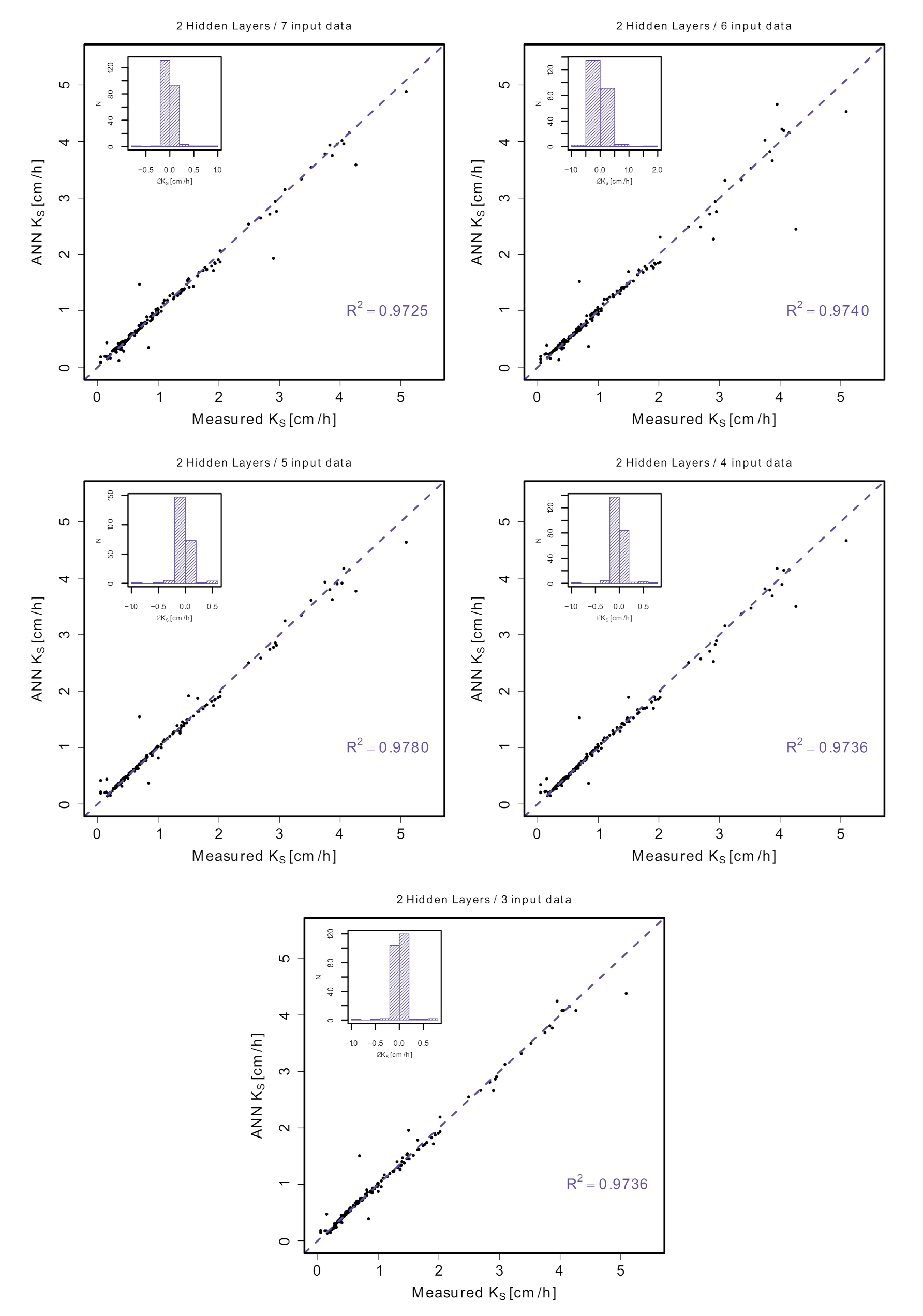
| 7-9-3-1 | 0.0459 | 0.0159 | 0.9725 | |
| 7 | 7-7-6-1 | 0.0460 | 0.0164 | 0.9720 |
| 7-10-4-1 | 0.0465 | 0.0162 | 0.9715 | |
| 6-5-7-1 | 0.0445 | 0.0171 | 0.9740 | |
| 6 | 6-6-3-1 | 0.0455 | 0.0171 | 0.9742 |
| 6-8-4-1 | 0.0447 | 0.0163 | 0.9739 | |
| 5-8-3-1 | 0.0413 | 0.0152 | 0.9780 | |
| 5 | 5-4-9-1 | 0.0417 | 0.0156 | 0.9774 |
| 5-8-8-1 | 0.0418 | 0.0152 | 0.9777 | |
| 4-9-10-1 | 0.0449 | 0.0152 | 0.9736 | |
| 4 | 4-8-8-1 | 0.0450 | 0.0156 | 0.9735 |
| 4-9-9-1 | 0.0452 | 0.0155 | 0.9734 | |
| 3-9-6-1 | 0.0433 | 0.0155 | 0.9757 | |
| 3 | 3-8-9-1 | 0.0434 | 0.0154 | 0.9757 |
| 3-8-6-1 | 0.0436 | 0.0160 | 0.9755 |
| Model | RMSE | Type | |
|---|---|---|---|
| This work | 0.0413 | 0.9780 | ANN |
| Tamari et al. [31] | 0.0707 | NA | ANN |
| Brakensiek et al. [9] | 0.1370 | 0.9953 | PTF |
| Erzin et al. [12] | 0.1700 | 0.9970 | ANN |
| Saxton et al. [32] | 0.1895 | 0.9915 | PTF |
| Parasuraman et al. [33] | 0.1900 | NA | ANN |
| Trejo-Alonso et al. [23] | 0.1983 | 0.9901 | PTF |
| Cosby et al. [34] | 0.4325 | 0.9546 | PTF |
| Ahuja et al. [35] | 0.6498 | 0.8910 | PTF |
| Schaap & Leij [36] | 0.7130 | NA | ANN |
| Vereecken et al. [37] | 0.7143 | 0.9307 | PTF |
| Minasny et al. [38] | 0.7330 | NA | ANN |
| Ferrer-Julià et al. [39] | 1.3018 | 0.4083 | PTF |
| Merdun et al. [40] | 3.5110 | 0.5240 | ANN |
Publisher’s Note: MDPI stays neutral with regard to jurisdictional claims in published maps and institutional affiliations. |
© 2021 by the authors. Licensee MDPI, Basel, Switzerland. This article is an open access article distributed under the terms and conditions of the Creative Commons Attribution (CC BY) license (http://creativecommons.org/licenses/by/4.0/).
Share and Cite
Trejo-Alonso, J.; Fuentes, C.; Chávez, C.; Quevedo, A.; Gutierrez-Lopez, A.; González-Correa, B. Saturated Hydraulic Conductivity Estimation Using Artificial Neural Networks. Water 2021, 13, 705. https://doi.org/10.3390/w13050705
Trejo-Alonso J, Fuentes C, Chávez C, Quevedo A, Gutierrez-Lopez A, González-Correa B. Saturated Hydraulic Conductivity Estimation Using Artificial Neural Networks. Water. 2021; 13(5):705. https://doi.org/10.3390/w13050705
Chicago/Turabian StyleTrejo-Alonso, Josué, Carlos Fuentes, Carlos Chávez, Antonio Quevedo, Alfonso Gutierrez-Lopez, and Brandon González-Correa. 2021. "Saturated Hydraulic Conductivity Estimation Using Artificial Neural Networks" Water 13, no. 5: 705. https://doi.org/10.3390/w13050705
APA StyleTrejo-Alonso, J., Fuentes, C., Chávez, C., Quevedo, A., Gutierrez-Lopez, A., & González-Correa, B. (2021). Saturated Hydraulic Conductivity Estimation Using Artificial Neural Networks. Water, 13(5), 705. https://doi.org/10.3390/w13050705