
Using Concentration–Discharge Relationships to Identify Influences on Surface and Subsurface Water Chemistry along a Watershed Urbanization Gradient


Abstract
1. Introduction
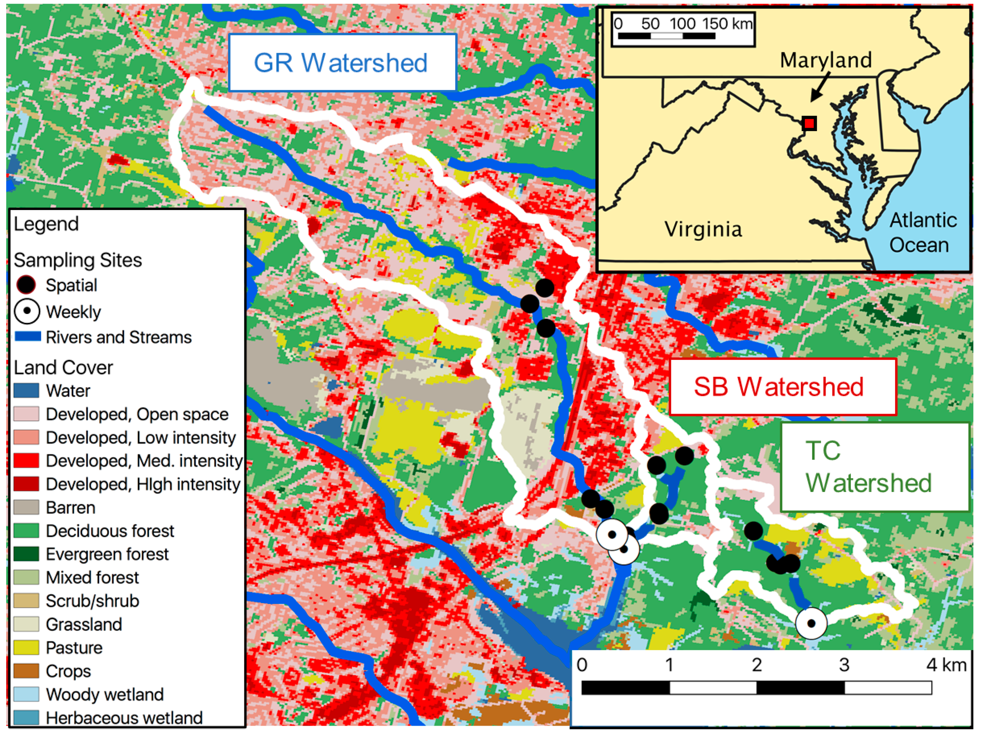
2. Methods
3. Results
3.1. Water Quality Variation among Stream Systems
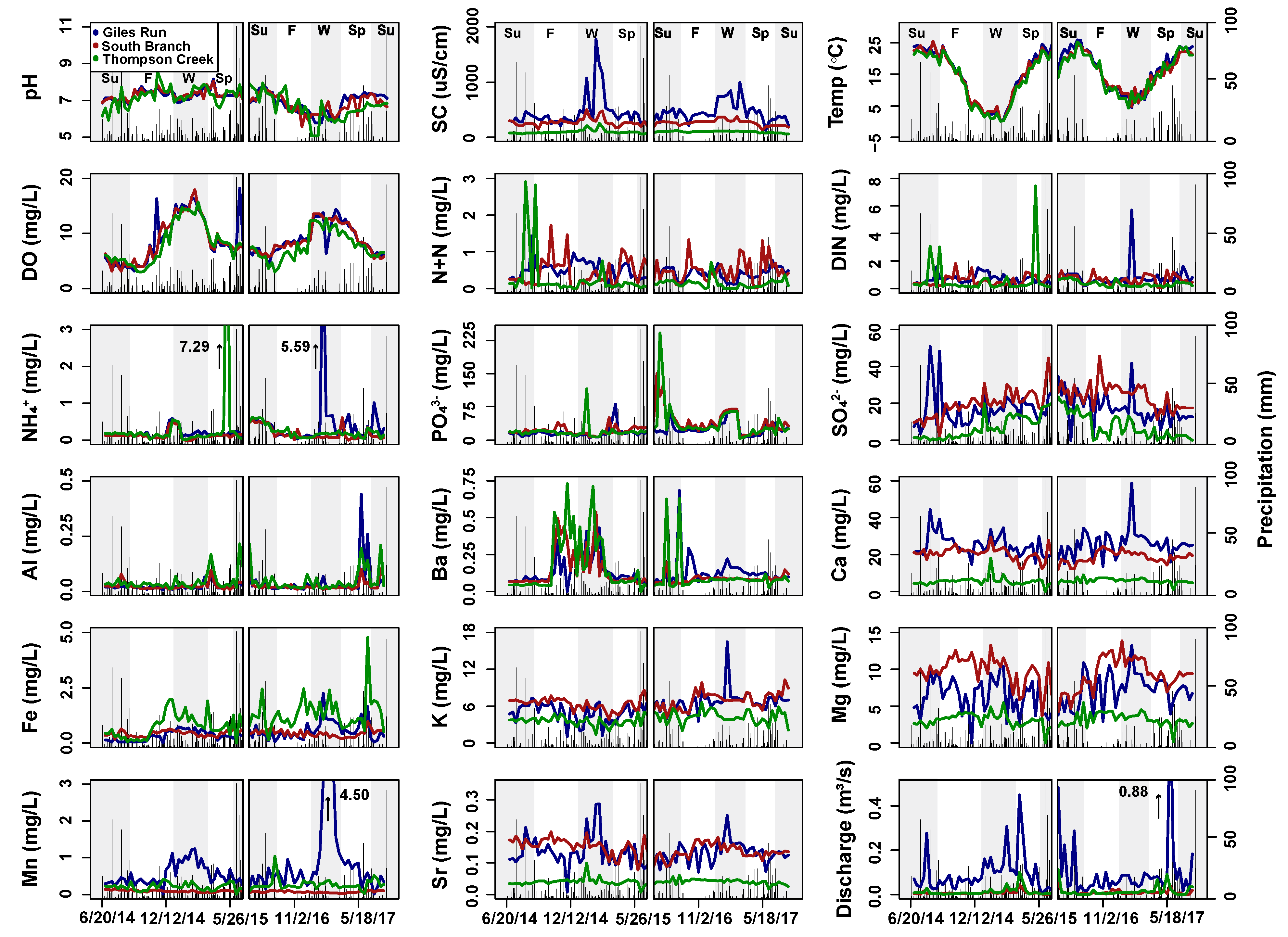
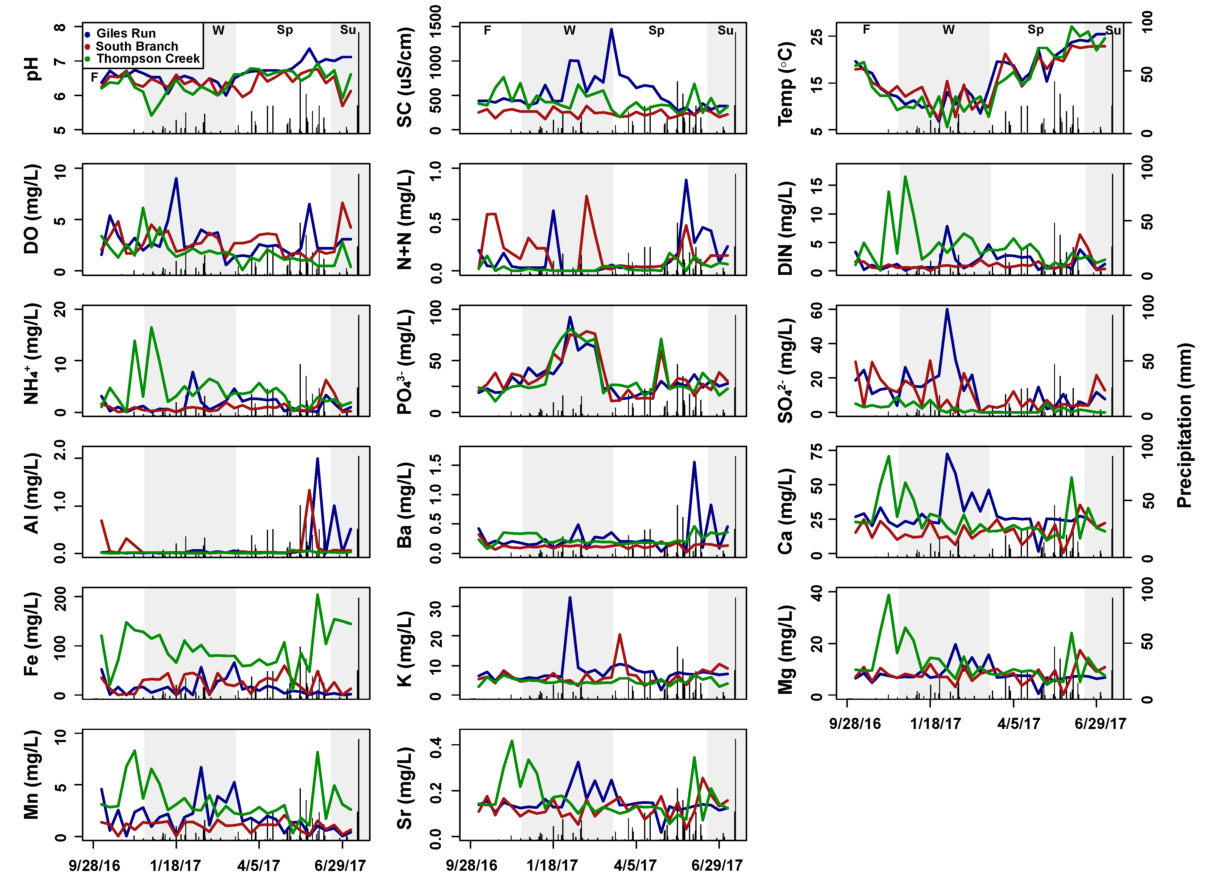
3.2. Variation in Discharge and Water Quality at Multiple Temporal Scales
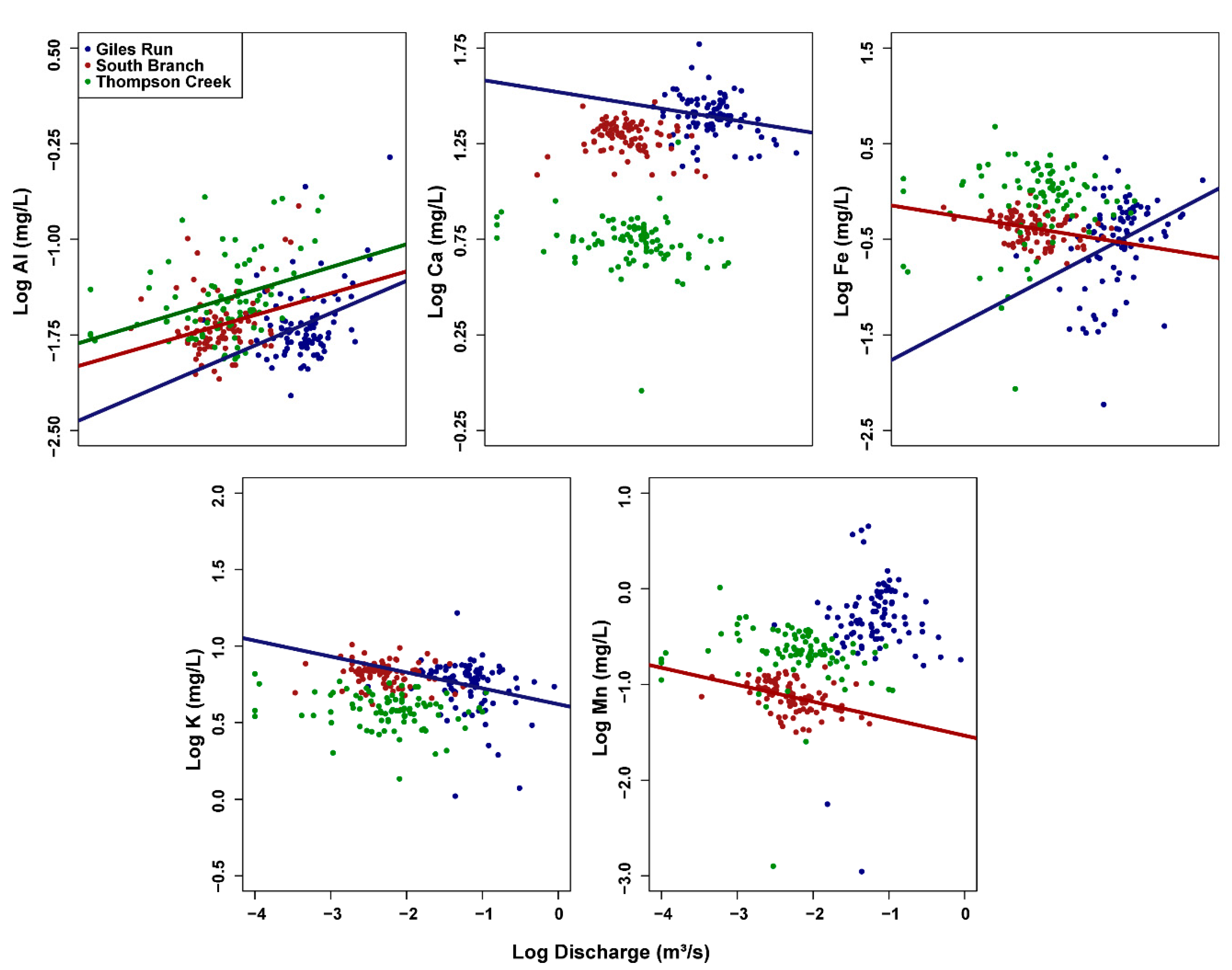
3.3. Concentration–Discharge (C–Q) Relationships
3.4. Correlations among Water Quality Variables
4. Discussion
4.1. Solute Sources and Transport across an Urbanization Gradient
4.2. Stream Health and Urban Stream Syndrome
4.3. Limitations of this Study and Future Research
4.4. Broader Relevance
Supplementary Materials
Author Contributions
Funding
Data Availability Statement
Acknowledgments
Conflicts of Interest
References
- Martinuzzi, S.; Januchowski-Hartley, S.R.; Pracheil, B.M.; McIntyre, P.B.; Platinga, A.J.; Lewis, D.J.; Radeloff, V.C. Threats and opportunities for freshwater conservation under future land use change scenarios in the United States. Glob. Chang. Biol. 2014, 20, 113–124. [Google Scholar] [CrossRef] [PubMed]
- Kaye, J.P.; Groffman, P.M.; Grimm, N.B.; Baker, L.A.; Pouyat, R.V. A distinct urban biogeochemistry? Trends Ecol. Evol. 2006, 21, 192–199. [Google Scholar] [CrossRef]
- Grimm, N.B.; Faeth, S.H.; Golubiewski, N.E.; Redman, C.L.; Wu, J.; Bai, X.; Briggs, J.M. Global change and the ecology of cities. Science 2008, 319, 756–760. [Google Scholar] [CrossRef]
- Yang, G.; Bowling, L.C.; Cherkauer, K.A.; Pijanowski, B.C.; Niyogi, D. Hydroclimatic response of watersheds to urban intensity: An observational and modeling-based analysis for the White River Basin, Indiana. J. Hydrometeorol. 2010, 11, 122–138. [Google Scholar] [CrossRef]
- Paul, M.J.; Meyer, J.L. Streams in the urban landscape. Annu. Rev. Ecol. Syst. 2001, 23, 333–365. [Google Scholar] [CrossRef]
- Walsh, C.J.; Roy, A.H.; Feminella, J.W.; Cottingham, P.D.; Groffman, P.M.; Morgan II, R.P. The urban stream syndrome: Current knowledge and the search for a cure. J. N. Am. Benthol. Soc. 2005, 24, 706–723. [Google Scholar] [CrossRef]
- Wenger, S.J.; Roy, A.H.; Rhett Jackson, C.; Bernhardt, E.S.; Carter, T.L.; Filoso, S.; Gibson, C.A.; Hession, W.C.; Kaushal, S.S.; Marti, E.; et al. Twenty-six key research questions in urban stream ecology: An assessment of the state of the science. J. N. Am. Benthol. Soc. 2009, 28, 1080–1098. [Google Scholar] [CrossRef]
- Konrad, C.P.; Booth, D.B. Hydrologic changes in urban streams and their ecological significance. Am. Fish. Soc. Symp. 2005, 47, 157–177. [Google Scholar]
- Jacobson, C.R. Identification and quantification of the hydrological impacts of imperviousness in urban catchments: A review. J. Environ. Manag. 2011, 92, 1438–1448. [Google Scholar] [CrossRef]
- Gomi, T.; Sidle, T.C.; Richarson, J.S. Understanding processes and downstream linkages of headwater systems. Bioscience 2002, 52, 905–916. [Google Scholar] [CrossRef]
- Leopold, L.B.; Huppman, R.; Miller, A. Geomorphic effects of urbanization in forty-one years of observation. Am. Philos. Soc. 2005, 149, 349–371. [Google Scholar]
- Kaushal, S.S.; Belt, K.T. The urban watershed continuum: Evolving spatial and temporal dimensions. Urban Ecosyst. 2012, 15, 409–435. [Google Scholar] [CrossRef]
- Schoonover, J.E.; Lockaby, B.G.; Pan, S. Changes in chemical and physical properties of stream water across an urban-rural gradient in western Georgia. Urban Ecosyst. 2005, 8, 107–124. [Google Scholar] [CrossRef]
- Cooper, C.A.; Mayer, P.M.; Faulkner, B.R. Effects of road salts on groundwater and surface water dynamics of sodium and chloride in an urban restored stream. Biogeochemistry 2014, 121, 149–166. [Google Scholar] [CrossRef]
- Kaushal, S.S.; Duan, S.; Doody, T.R.; Haq, S.; Smith, R.M.; Newcomer Johnson, T.A.; Newcomb, K.D.; Gorman, J.; Bowman, N.; Mayer, P.M.; et al. Human-accelerated weathering increases salinization, major ions, and alkalinization in freshwater across land use. Appl. Geochem. 2017, 83, 121–135. [Google Scholar] [CrossRef]
- Coleman II, J.C.; Miller, M.C.; Mink, F.L. Hydrologic disturbance reduces biological integrity in urban streams. Environ. Monit. Assess. 2011, 172, 663–687. [Google Scholar] [CrossRef]
- South, E.J.; Ensign, W.E. Life history of Campostoma oligolepsis (largescale stoneroller) in urban and rural streams. Southeast. Nat. 2013, 12, 781–789. [Google Scholar] [CrossRef]
- Ledford, S.H.; Lautz, L.K.; Vidon, P.; Stella, J.C. Impact of seasonal changes in stream metabolism on nitrate concentrations in an urban stream. Biogeochemistry 2017, 133, 317–331. [Google Scholar] [CrossRef]
- Roy, J.W.; Bickerton, G. Toxic groundwater contaminants: An overlooked contributor to Urban Stream Syndrome. Environ. Sci. Technol. 2012, 46, 729–736. [Google Scholar] [CrossRef]
- Hancock, P.J. Human impacts on the stream-groundwater exchange zone. Environ. Manag. 2002, 29, 763–781. [Google Scholar] [CrossRef]
- Lawrence, J.E.; Skold, M.E.; Hussain, F.A.; Silverman, D.R.; Resh, V.H.; Sedlak, D.L.; Luthy, R.G.; McCray, J.E. Hyporheic zone in urban streams: A review and opportunities for enhancing water quality and improving aquatic habitat by active management. Environ. Eng. Sci. 2013, 30, 480–500. [Google Scholar] [CrossRef]
- Merill, L.; Tonjes, D.J. A review of the hyporheic zone, stream restoration, and means to enhance denitrification. Crit. Rev. Environ. Sci. Technol. 2014, 44, 2337–2379. [Google Scholar] [CrossRef]
- Elmore, A.J.; Kaushal, S.S. Disappearing headwaters: Patterns of stream burial due to urbanization. Front. Ecol. Environ. 2008, 6, 308–312. [Google Scholar] [CrossRef]
- Groffman, P.M.; Boulware, N.J.; Zipperer, W.C.; Pouyat, R.V.; Band, L.E.; Colosimo, M.F. Soil nitrogen cycle processes in urban riparian zones. Environ. Sci. Technol. 2002, 36, 4547–4552. [Google Scholar] [CrossRef]
- Hardison, E.C.; O’Driscoll, M.A.; DeLoatch, J.P.; Howard, R.J.; Brinson, M.M. Urban land use, channel incision, and water table decline along coastal plain streams, North Carolina. J. Am. Water Resour. Assoc. 2009, 45, 1032–1046. [Google Scholar] [CrossRef]
- Price, E.L.; Peric, M.S.; Romero, G.Q.; Kratina, P. Land use alters trophic redundancy and resource flow through stream food webs. J. Anim. Ecol. 2018, 88, 677–689. [Google Scholar] [CrossRef]
- Moatar, F.; Abbott, B.W.; Minaudo, C.; Curie, F.; Pinay, G. Elemental properties, hydrology, and biology interact to shape concentration-discharge curves for carbon, nutrients, sediment, and major ions. Water Resour. Res. 2017, 53, 1270–1287. [Google Scholar] [CrossRef]
- Godsey, S.E.; Kirchner, J.W.; Clow, D.W. Concentration-discharge relationships reflect chemostatic characteristics of US catchments. Hydrol. Process. 2009, 23, 1844–1864. [Google Scholar] [CrossRef]
- Underwood, K.L.; Rizzo, D.M.; Schroth, A.W.; Dewoolkar, M.M. Evaluating spatial variability in sediment and phosphorus concentration-discharge relationships using Bayesian inference and self-organizing maps. Water Resour. Res. 2017, 53, 10293–10316. [Google Scholar] [CrossRef]
- Zhang, Q.; Harman, C.J.; Ball, W.P. An improved method for interpretation of riverine concentration-discharge relationships indicates long-term shifts in res-ervoir sediment trapping. Geophys. Res. Lett. 2016, 43, 10–215. [Google Scholar] [CrossRef]
- Hunsaker, C.T.; Johnson, D.W. Concentration-discharge relationships in headwater streams of the Sierra Nevada, California. Water Resour. Res. 2017, 53, 7869–7884. [Google Scholar] [CrossRef]
- Chorover, J.; Derry, L.A.; McDowell, W.H. Concentration-discharge relations in the critical zone: Implications for resolving critical zone structure, function, and evolution. Water Resour. Res. 2017, 53, 8654–8659. [Google Scholar] [CrossRef]
- USGS. The StreamStats Program. Available online: http://streamstats.usgs.gov (accessed on 26 February 2021).
- Gore, J.A. Discharge measurements and streamflow analysis. In Methods in Stream Ecology, 2nd ed.; Hauer, F.R., Lamberti, G.A., Eds.; Lamberti Academic Press: Cambridge, MA, USA, 2007; pp. 51–78. [Google Scholar]
- Miller, R.G.; Kopfler, F.C.; Kelty, K.C.; Stober, J.A.; Ulmer, N.S. The occurrence of aluminum in drinking water. J. Am. Water Work. Assoc. 1984, 76, 84–91. [Google Scholar] [CrossRef]
- Boulton, A.J.; Findlay, S.; Marmonier, P.; Stanley, E.H.; Valett, H.M. The functional significance of the hyporheic zone in streams and rivers. Annu. Rev. Ecol. Evol. Syst. 1998, 29, 58–81. [Google Scholar] [CrossRef]
- Howarth, R.; Swaney, D.; Billen, G.; Gardiner, J.; Hong, B.; Humborg, C.; Johnes, P.; Morth, C.-M.; Marino, R. Nitrogen fluxes from the landscape are controlled by net anthropogenic nitrogen inputs and by climate. Front. Ecol. Environ. 2012, 10, 37–43. [Google Scholar] [CrossRef]
- Jordan, T.E.; Correll, D.L.; Weller, D.E. Relating nutrient discharges from watersheds to land use and streamflow variability. Water Resour. Res. 1997, 33, 2579–2590. [Google Scholar] [CrossRef]
- David, M.B.; Drinkwater, L.E.; McIsaac, G.F. Sources of nitrate yields in the Mississippi River Basin. J. Environ. Qual. 2010, 39, 1657–1667. [Google Scholar] [CrossRef]
- Jordan, T.E.; Weller, D.E.; Correll, D.L. Sources of nutrient inputs to the Patuxent River Estuary. Estuaries 2003, 26, 226–243. [Google Scholar] [CrossRef]
- Mayer, P.M.; Groffman, P.M.; Striz, E.A.; Kaushal, S.S. Nitrogen dynamics at the groundwater-surface water interface of a degraded stream. J. Environ. Qual. 2010, 39, 810–823. [Google Scholar] [CrossRef] [PubMed]
- Donn, M.J.; Barron, O.V. Biogeochemical processes in the groundwater discharge zone of urban streams. Biogeochemistry 2013, 115, 267–286. [Google Scholar] [CrossRef]
- Horswell, J.; Prosser, J.A.; Siggins, A.; van Schaik, A.; Ying, L.; Ross, C.; McGill, A.; Northcott, G. Assessing the impacts of chemical cocktails on the soil ecosystem. Soil Biol. Biochem. 2014, 75, 64–72. [Google Scholar] [CrossRef]
- Bernhardt, E.S.; Rosi, E.J.; Gessner, M.O. Synthetic chemicals as agents of global change. Front. Ecol. Environ. 2017, 15, 84–90. [Google Scholar] [CrossRef]
- Kaushal, S.S.; Gold, A.J.; Bernal, S.; Newcomer Johnson, T.A.; Addy, K.; Burgin, A.; Burns, D.A.; Coble, A.A.; Hood, E.; Lu, Y.; et al. Watershed ‘chemical cocktails’: Forming novel elemental combinations in Anthropocene fresh waters. Biogeochemistry 2018, 141, 281–305. [Google Scholar] [CrossRef]
- Kaushal, S.S.; Likens, G.E.; Pace, M.L.; Haq, S.; Wood, K.L.; Galella, J.G.; Morel, C.; Doody, T.R.; Wessel, B.; Kortelainen, P.; et al. Novel ‘chemical cocktails’ in inland waters are a consequence of the freshwater salinization syndrome. Philos. Trans. R. Soc. B 2019, 374, 1–11. [Google Scholar] [CrossRef]
- Hooper, R.P.; Christopherson, N.; Peters, N.E. Modelling streamwater chemistry as a mixture of soil water end-members—An application to the Panola Mountain Catch-ment, Georgia, USA. J. Hydrol. 1990, 116, 321–343. [Google Scholar] [CrossRef]
- Rose, S. Comparative major ion geochemistry of Piedmont streams in the Atlanta, Georgia region: Possible effects of urbanization. Environ. Geol. 2002, 42, 102–113. [Google Scholar] [CrossRef]
- Puckett, L.J.; Bricker, O.P. Factors controlling the major ion chemistry of streams in the Blue Ridge valley and ridge physiographic provinces of Virginia and Maryland. Hydrol. Process. 1992, 6, 79–98. [Google Scholar] [CrossRef]
- Groffman, P.M.; Law, N.L.; Belt, K.T.; Band, L.E.; Fisher, G.T. Nitrogen fluxes and retention in urban watershed ecosystems. Ecosystems 2004, 7, 393–403. [Google Scholar] [CrossRef]
- Arnold, C.L.; Gibbons, C.J. Impervious surface coverage: The emergence of a key environmental indicator. J. Am. Plan. Assoc. 1996, 62, 243–258. [Google Scholar] [CrossRef]
- Chang, H.; Carlson, T.N. Water quality during winter storm events in Spring Creek, Pennsylvania USA. Hydrobiologia 2005, 544, 321–332. [Google Scholar] [CrossRef]
- Gardner, K.M.; Royer, T.V. Effect of road salt application on seasonal chloride concentrations and toxicity in South-Central Indiana streams. J. Environ. Qual. 2010, 39, 1036–1042. [Google Scholar] [CrossRef]
- Howard, K.W.F.; Hayes, J. Groundwater contamination due to road deicing chemicals—Salt balance implications. Geosci. Can. 1993, 20, 1–8. [Google Scholar]
- Moore, J.; Fanelli, R.M.; Sekellick, A.J. High-frequency data reveal deicing salts drive elevated specific conductance and chloride along with pervasive and frequent exceedances of the U.S. Environmental Protection Agency Aquatic Life Criteria for chloride in urban streams. Environ. Sci. Technol. 2020, 54, 778–789. [Google Scholar] [CrossRef]
- Corsi, S.R.; Graczyk, D.J.; Geis, S.W.; Booth, N.L.; Richards, K.D. A fresh look at road salt: Aquatic toxicity and water-quality impacts on local, regional, and national scales. Environ. Sci. Technol. 2010, 44, 7376–7382. [Google Scholar] [CrossRef] [PubMed]
- Canedo-Arguelles, M.; Kefford, B.J.; Piscard, C.; Prat, N.; Shafer, R.B.; Shulz, C. Salination of rivers: An urgent ecological issue. Environ. Pollut. 2013, 173, 157–167. [Google Scholar] [CrossRef]
- Hintz, W.D.; Relyea, R.A. Impacts of road deicing salts on the early-life growth and development of a stream salmonid: Salt type matters. Environ. Pollut. 2017, 223, 409–415. [Google Scholar] [CrossRef]
- USEPA. Ambient Water Quality Criteria Recommendations: Information Supporting the Development of State and Tribal Nutrient Criteria for Rivers and Streams in Nutrient Ecoregion I. 2001; p. 125. [Google Scholar]
- Line, D.E.; White, N.M.; Osmond, D.L.; Jennings, G.D.; Mojonnier, C.B. Pollutant export from various land uses in the Upper Neuse River Basin. Water Environ. Res. 2002, 74, 100–108. [Google Scholar] [CrossRef]
- Connor, N.P.; Sarraino, S.; Frantz, D.E.; Bushaw-Newton, K.; MacAvoy, S.E. Geochemical characteristics of an urban river: Influences of an anthropogenic landscape. Appl. Geochem. 2014, 47, 209–216. [Google Scholar] [CrossRef]
- Wang, W. Site-specific barium toxicity to common duckweed, Lemna minor. Aquat. Toxicol. 1988, 12, 203–212. [Google Scholar] [CrossRef]
- Cadmus, P.; Brinkman, S.F.; May, M.K. Chronic toxicity of ferric iron for North American aquatic organisms: Derivation of a chronic water quality criterion using single species and mesocosm data. Arch. Environ. Contam. Toxicol. 2018, 74, 605–615. [Google Scholar] [CrossRef]
- Lasier, P.J.; Winger, P.V.; Bogenrieder, K.J. Toxicity of manganese to Ceriodaphnia dubia and Hyalella azteca. Arch. Environ. Contam. Toxicol. 2000, 38, 298–304. [Google Scholar] [CrossRef]
- Peters, A.; Lofts, S.; Merrington, G.; Brown, B.; Stubblefield, W.; Harlow, K. Development of biotic ligand models for chronic manganese toxicity to fish, invertebrates, and algae. Environ. Toxicol. Chem. 2011, 30, 2407–2415. [Google Scholar] [CrossRef] [PubMed]
- McPherson, C.A.; Lawrence, G.S.; Elphick, J.R.; Chapman, P.M. Development of a strontium chronic effects benchmark for aquatic life in freshwater. Environ. Toxicol. Chem. 2014, 33, 2472–2478. [Google Scholar] [CrossRef] [PubMed]
- Booth, D.B.; Roy, A.H.; Smith, B.; Capps, K.A. Global perspectives on the urban stream syndrome. Freshw. Sci. 2016, 35, 412–420. [Google Scholar] [CrossRef]
- Volk, J.A.; Savidge, K.B.; Scudlark, J.R.; Andres, A.S.; Ullman, W.J. Nitrogen loads through baseflow, stormflow, and underflow to Rehoboth Bay, Delaware. J. Environ. Qual. 2006, 35, 1742–1755. [Google Scholar] [CrossRef]
- Janke, B.D.; Finlay, J.C.; Hobbie, S.E.; Baker, L.A.; Stener, R.W.; Nidzgorski, D.; Wilson, B.N. Contrasting influences of stormflow and baseflow pathways on nitrogen and phosphorus export from an urban watershed. Biogeochemistry 2014, 121, 209–228. [Google Scholar] [CrossRef]
- Du, J.; Feng, H.; Nie, J.; Li, Y.; Witherell, B.B. Characterisation and assessment of spatiotemporal variations in nutrient concentrations and fluxes in an urban watershed: Passaic River Basin, New Jersey, USA. Int. J. Environ. Pollut. 2018, 63, 154–177. [Google Scholar] [CrossRef]
- Seto, K.C.; Fragkias, M.; Guneralp, B.; Reilly, M.K. A meta-analysis of global urban land expansion. PLoS ONE 2011, 6, e23777. [Google Scholar] [CrossRef]
- Morgan, C.; Owens, N. Benefits of water quality policies: The Chesapeake Bay. Ecol. Econ. 2001, 39, 271–284. [Google Scholar] [CrossRef]
- Paolisso, M. Blue crabs and controversy on the Chesapeake Bay: A cultural model for understanding waterman’s reasoning about blue crab management. Hum. Organ. 2002, 61, 226–239. [Google Scholar] [CrossRef]
- Lipton, D. The value of improved water quality to the Chesapeake Bay Boaters. Mar. Resour. Econ. 2004, 19, 265–270. [Google Scholar] [CrossRef]
- Walsh, P.; Griffiths, C.; Guignet, D.; Klemick, H. Modeling the property price impact of water quality in 14 Chesapeake Bay counties. Ecol. Econ. 2017, 135, 103–113. [Google Scholar] [CrossRef]
- Boesch, D.F.; Brinsfield, R.B.; Magnien, R.E. Chesapeake Bay eutrophication. J. Environ. Qual. 2001, 30, 303–320. [Google Scholar] [CrossRef]
- Kemp, W.M.; Boynton, W.R.; Adolf, J.E.; Boesch, D.F.; Boicourt, W.C.; Brush, G.; Cornwell, J.C.; Fisher, T.R.; Glibert, P.M.; Hagy, J.D.; et al. Eutrophication of Chesapeake Bay: Historical trends and ecological interactions. Mar. Ecol. Prog. Ser. 2005, 303, 1–29. [Google Scholar] [CrossRef]
- Fisher, T.R.; Hagy III, J.D.; Boynton, W.R.; Williams, M.R. Hydrology and chemistry of the Choptank basin. Water Air Soil Pollut. 2006, 105, 387–397. [Google Scholar] [CrossRef]
- Reay, W.G.; Gallagher, D.L.; Simmons Jr., G. M. Groundwater discharge and its impact on surface water quality in a Chesapeake Bay inlet. Water Resour. Bull. 1992, 28, 1121–1134. [Google Scholar] [CrossRef]
- Shields, C.A.; Band, L.E.; Law, N.L.; Groffman, P.M.; Kaushal, S.S.; Savvas, K.; Fisher, G.T.; Belt, K.T. Streamflow distribution of non-point source nitrogen export from urban-rural catchments in the Chesapeake Bay watershed. Water Resour. Res. 2008, 44, W09416. [Google Scholar] [CrossRef]
- Bhaskar, A.S.; Beesley, L.; Burns, M.J.; Fletcher, T.D.; Hamel, P.; Oldham, C.E.; Roy, A.H. Will it rise or will it fall? Managing the complex effects of urbanization on base flow. Freshw. Sci. 2015, 35, 293–310. [Google Scholar] [CrossRef]


| Giles Run (GR) | South Branch (SB) | Thompson Creek (TC) | |
|---|---|---|---|
| Watershed Area (km2) | 13.05 | 1.42 | 2.75 |
| Impervious Surface Coverage (%) | 18.5 | 6.21 | 1.23 |
| Total Developed (%) | 66.1 | 31.7 | 14.2 |
| Forested or Natural (%) | 25.4 | 62.5 | 64.5 |
| Estimated Runoff Ratio (m3s−1mm−1) ± SEM | 0.19 ± 0.07 | 0.02 ± 0.01 | 0.02 ± 0.01 |
| Surface Water | Subsurface Water | |||||
|---|---|---|---|---|---|---|
| Variable | GR | SB | TC | GR | SB | TC |
| Discharge (m3s−1) | 0.10 (0.0–0.89) | 0.01 (0.0–0.06) | 0.01 (0.0–0.11) | N/A | N/A | N/A |
| Temp (°C) | 15.5 (0.2–26) | 14.9 (0.1–26) | 14.3 (0.1–25) | 17.3 (6.8–25) | 16.8 (7.3–24) | 16.6 (5.6–27) |
| DO (mg L−1) | 8.8 (3.2–18) | 8.8 (3.2–18) | 8.0 (3.0–16) | 2.8 (0.6–9.0) | 2.7 (1.0–6.6) | 1.7 (0.1–6.1) |
| PH | 7.1 (5.8–8.2) | 7.1 (5.6–8.0) | 6.9 (5.1–8.5) | 6.7 (6.0–7.4) | 6.5 (5.7–7.2) | 6.4 (5.4–6.9) |
| SC (µS cm−1) | 450 (120–1780) | 270 (130–500) | 98.4 (60.0–260) | 510 (210–1460) | 250 (160–440) | 440 (190–880) |
| N+N (mg N L−1) | 0.5 (0.1–1.4) | 0.5 (0.0–1.7) | 0.2 (0.0–2.9) | 0.1 (0.0–0.9) | 0.2 (0.0–0.7) | 0.04 (0.0–0.17) |
| NH4+ (mg N L−1) | 0.3 (0.0–5.6) | 0.2 (0.0–0.6) | 0.3 (0.0–7.3) | 1.5 (0.0–7.8) | 1.0 (0.0–6.3) | 4.0 (0.1–17) |
| PO43− (µg P L−1) | 21.5 (4.2–81) | 31 (6.0–150) | 28.2 (3.7–242) | 32.3 (13–92) | 34.9 (11–79) | 33.8 (11–81) |
| SO42− (mg S L−1) | 17.1 (0.0–50.9) | 21.9 (2.0–45.8) | 7.1 (0.0–23.4) | 11.9 (0.0–60) | 10.0 (0.0–30) | 1.9 (0.0–8.9) |
| Al (mg Al L−1) | 0.0 (0.0–0.4) | 0.0 (0.0–0.2) | 0.1 (0.0–0.2) | 0.2 (0.0–3.0) | 0.2 (0.0–2.0) | 0.0 (0.0–0.1) |
| Ba (mg Ba L−1) | 0.1 (0.0–0.7) | 0.1 (0.1–0.5) | 0.1 (0.0–0.7) | 0.3 (0.0–1.6) | 0.1 (0.0–0.3) | 0.2 (0.1–0.5) |
| Ca (mg Ca L−1) | 25.4 (13.5–59) | 19.6 (12.0–30) | 5.6 (0.0–18) | 30 (1.3–73) | 17.1 (0.5–43) | 24.6 (9.4–71) |
| Fe (mg Fe L−1) | 0.4 (0.0–2.3) | 0.4 (0.2–1.0) | 1.1 (0.0–4.8) | 13.6 (0.0–66) | 23.5 (0.1–60) | 94.4 (10.3–204) |
| K (mg K L−1) | 5.9 (1.1–17) | 6.7 (3.9–10.2) | 3.9 (1.4–6.6) | 7.9 (1.7–33) | 6.3 (3.1–20) | 4.6 (2.8–6.8) |
| Mg (mg Mg L−1) | 6.8 (0.0–13) | 9.5 (3.7–14) | 3.2 (0.0–5.5) | 8.0 (0.5–20) | 8.5 (0.2–19) | 12.1 (4.0–39) |
| Mn (mg Mn L−1) | 0.7 (0.0–4.5) | 0.1 (0.0–0.2) | 0.2 (0.0–1.0) | 1.8 (0.0–6.7) | 1.0 (0.0–2.1) | 3.3 (0.3–8.3) |
| Sr (mg Sr L−1) | 0.1 (0.0–0.3) | 0.1 (0.1–0.3) | 0.0 (0.0–0.1) | 0.1 (0.0–0.3) | 0.1 (0.0–0.3) | 0.2 (0.1–0.4) |
| Variable | Type | DO | pH | SC | N+N | NH4+ | PO43− | SO42− | ||||||||||||||
|---|---|---|---|---|---|---|---|---|---|---|---|---|---|---|---|---|---|---|---|---|---|---|
| Temp | SW | - | - | - | 0 | 0 | 0 | - | - | - | 0 | 0 | + | 0 | + | + | 0 | + | + | 0 | - | 0 |
| HZ | 0 | 0 | - | + | + | + | - | 0 | 0 | + | 0 | + | 0 | 0 | - | - | 0 | 0 | - | 0 | 0 | |
| DO | SW | - | 0 | 0 | 0 | + | + | + | 0 | 0 | 0 | 0 | - | - | 0 | - | 0 | 0 | + | + | ||
| HZ | - | 0 | - | - | 0 | 0 | 0 | 0 | 0 | - | - | - | 0 | + | 0 | 0 | + | + | 0 | |||
| pH | SW | - | - | - | - | 0 | 0 | 0 | 0 | 0 | 0 | 0 | - | 0 | 0 | 0 | 0 | + | ||||
| HZ | - | - | - | + | 0 | + | 0 | 0 | 0 | 0 | 0 | 0 | 0 | 0 | - | 0 | - | |||||
| SC | SW | - | - | - | 0 | 0 | 0 | + | 0 | 0 | 0 | 0 | 0 | + | + | + | ||||||
| HZ | - | - | - | - | 0 | 0 | + | 0 | 0 | 0 | 0 | 0 | 0 | 0 | 0 | |||||||
| N+N | SW | - | - | - | - | 0 | 0 | + | - | 0 | 0 | 0 | + | 0 | ||||||||
| HZ | - | - | - | - | 0 | - | - | 0 | 0 | 0 | 0 | 0 | 0 | |||||||||
| NH4+ | SW | - | - | - | - | - | 0 | 0 | 0 | 0 | 0 | 0 | ||||||||||
| HZ | - | - | - | - | - | 0 | 0 | + | 0 | - | 0 | |||||||||||
| PO43− | SW | - | - | - | - | - | - | 0 | + | 0 | ||||||||||||
| HZ | - | - | - | - | - | - | + | 0 | 0 | |||||||||||||
| Variable | Type | SO42− | Al | Ba | Ca | Fe | K | Mg | Mn | Sr | ||||||||||||||||||
|---|---|---|---|---|---|---|---|---|---|---|---|---|---|---|---|---|---|---|---|---|---|---|---|---|---|---|---|---|
| pH | SW | 0 | 0 | + | 0 | 0 | 0 | 0 | 0 | 0 | - | 0 | 0 | 0 | 0 | 0 | - | - | - | - | - | - | - | + | - | - | 0 | 0 |
| HZ | - | 0 | - | 0 | 0 | 0 | 0 | 0 | 0 | - | 0 | 0 | - | 0 | 0 | 0 | 0 | 0 | - | 0 | 0 | - | 0 | 0 | - | 0 | 0 | |
| SO42− | SW | - | + | 0 | 0 | 0 | 0 | 0 | 0 | 0 | 0 | 0 | 0 | + | 0 | 0 | 0 | 0 | 0 | 0 | 0 | - | 0 | 0 | 0 | 0 | ||
| HZ | - | 0 | 0 | 0 | 0 | - | 0 | 0 | 0 | 0 | 0 | 0 | - | 0 | 0 | 0 | 0 | 0 | 0 | 0 | 0 | 0 | 0 | 0 | 0 | |||
| Al | SW | - | - | - | 0 | - | - | - | - | + | 0 | 0 | 0 | 0 | 0 | - | - | - | 0 | 0 | - | - | - | - | ||||
| HZ | - | - | + | + | + | 0 | 0 | 0 | 0 | 0 | 0 | + | 0 | 0 | 0 | 0 | 0 | 0 | 0 | 0 | 0 | 0 | 0 | |||||
| Ba | SW | - | - | - | + | + | + | + | 0 | + | 0 | + | 0 | + | + | + | + | 0 | + | + | + | + | ||||||
| HZ | - | - | - | + | + | 0 | + | + | + | 0 | 0 | 0 | + | + | + | + | + | + | + | + | + | |||||||
| Ca | SW | - | - | - | - | 0 | 0 | + | + | + | + | + | + | + | + | + | + | + | + | + | ||||||||
| HZ | - | - | - | - | 0 | 0 | + | + | + | + | + | + | + | + | 0 | + | + | + | + | |||||||||
| Fe | SW | - | - | - | - | - | 0 | 0 | 0 | 0 | 0 | 0 | + | + | + | 0 | 0 | 0 | ||||||||||
| HZ | - | - | - | - | - | 0 | - | 0 | 0 | 0 | + | + | + | + | + | 0 | + | |||||||||||
| K | SW | - | - | - | - | - | - | + | + | + | 0 | 0 | 0 | + | + | 0 | ||||||||||||
| HZ | - | - | - | - | - | - | + | + | + | 0 | 0 | + | + | + | 0 | |||||||||||||
| Mg | SW | - | - | - | - | - | - | - | + | 0 | + | + | + | + | ||||||||||||||
| HZ | - | - | - | - | - | - | - | + | 0 | + | + | + | + | |||||||||||||||
| Mn | SW | - | - | - | - | - | - | - | - | + | + | + | ||||||||||||||||
| HZ | - | - | - | - | - | - | - | - | + | 0 | + | |||||||||||||||||
| Variable | Giles Run (GR) | South Branch (SB) | Thompson Creek (TC) |
|---|---|---|---|
| Temp | 0.90 † | 0.84 † | 0.85 † |
| DO | −0.11 | 0.12 | 0.28 |
| pH | 0.80 † | 0.42 * | 0.29 |
| SC | 0.73 † | 0.17 | 0.20 |
| N+N | 0.44 * | −0.15 | 0.19 |
| NH4+ | 0.64 † | 0.27 | −0.12 |
| PO43− | 0.79 † | 0.63 † | 0.50 ** |
| SO42− | 0.60 † | 0.19 | 0.39 * |
| Al | 0.21 | 0.17 | 0.36 * |
| Ba | 0.11 | 0.025 | 0.035 |
| Ca | 0.56 † | −0.29 | 0.45 * |
| Fe | 0.16 | 0.047 | 0.39 * |
| K | 0.58 † | 0.45 * | 0.43 * |
| Mg | 0.68 † | −0.27 | 0.47 ** |
| Mn | 0.52 ** | 0.073 | 0.22 |
| Sr | 0.72 † | −0.41 * | 0.34 |
Publisher’s Note: MDPI stays neutral with regard to jurisdictional claims in published maps and institutional affiliations. |
© 2021 by the authors. Licensee MDPI, Basel, Switzerland. This article is an open access article distributed under the terms and conditions of the Creative Commons Attribution (CC BY) license (http://creativecommons.org/licenses/by/4.0/).
Share and Cite
Balerna, J.A.; Melone, J.C.; Knee, K.L. Using Concentration–Discharge Relationships to Identify Influences on Surface and Subsurface Water Chemistry along a Watershed Urbanization Gradient. Water 2021, 13, 662. https://doi.org/10.3390/w13050662
Balerna JA, Melone JC, Knee KL. Using Concentration–Discharge Relationships to Identify Influences on Surface and Subsurface Water Chemistry along a Watershed Urbanization Gradient. Water. 2021; 13(5):662. https://doi.org/10.3390/w13050662
Chicago/Turabian StyleBalerna, Jessica A., Jacob C. Melone, and Karen L. Knee. 2021. "Using Concentration–Discharge Relationships to Identify Influences on Surface and Subsurface Water Chemistry along a Watershed Urbanization Gradient" Water 13, no. 5: 662. https://doi.org/10.3390/w13050662
APA StyleBalerna, J. A., Melone, J. C., & Knee, K. L. (2021). Using Concentration–Discharge Relationships to Identify Influences on Surface and Subsurface Water Chemistry along a Watershed Urbanization Gradient. Water, 13(5), 662. https://doi.org/10.3390/w13050662