Evaluating Traditional Empirical Models and BPNN Models in Monitoring the Concentrations of Chlorophyll-A and Total Suspended Particulate of Eutrophic and Turbid Waters

Abstract

In order to use in situ sensed reflectance to monitor the concentrations of chlorophyll-a (Chl-a) and total suspended particulate (TSP) of waters in the Pearl River Delta, which is featured by the highly developed network of rivers, channels and ponds, 135 sets of simultaneously collected water samples and reflectance were used to test the performance of the traditional empirical models (band ratio, three bands) and the machine learning models of a back-propagation neural network (BPNN). The results of the laboratory analysis with the water samples show that the Chl-a ranges from 3 to 256 µg·L⁻¹ with an average of 39 µg·L⁻¹ while the TSP ranges from 8 to 162 mg·L⁻¹ and averages 42.5 mg·L⁻¹. Ninety sets of 135 samples are used as training data to develop the retrieval models, and the remaining ones are used to validate the models. The results show that the proposed band ratio models, the three-band combination models, and the corresponding BPNN models are generally successful in estimating the Chl-a and the TSP, and the mean relative error (MRE) can be lower than 30% and 25%, respectively. However, the BPNN models have no better performance than the traditional empirical models, e.g., in the estimation of TSP on the basis of the reflectance at 555 and 750 nm (R555 and R750, respectively), the model of BPNN (R555, R750) has an MRE of 23.91%, larger than that of the R750/R555 model. These results suggest that these traditional empirical models are usable in monitoring the optically active water quality parameters of Chl-a and TSP for eutrophic and turbid waters, while the machine learning models have no significant advantages, especially when the cost of training samples is considered. To improve the performance of machine learning models in future applications on the basis of ground sensor networks, large datasets covering various water situations and optimization of input variables of band configuration should be strengthened.

1. Introduction

Chlorophyll-a (Chl-a) and total suspended particulate (TSP) are two important parameters to assess water quality. Chl-a can be used as a proxy of the algae-associated primary productivity and the eutrophication status of water body. TSP is a major factor impacting the water turbidity, the transparency and the associated parameters of the aquatic environment. The traditional measurements of Chl-a and TSP are time-consuming and laborious, which hardly meets the demand of rapid monitoring. Remote sensing methods, based on the relationship between the remote sensing reflectance and water quality parameters, have advantages over traditional monitoring methods in terms of temporal and spatial scale [1,2].

Various traditional empirical models based on statistical regression and reflectance features have been developed to monitor optically active water parameters, e.g., Chl-a and TSP. Single-band models based on the correlation between the reflectance at a given wavelength and the water quality parameters [3,4]; two-band models based on the ratio of the peak reflectance to the valley [5,6] and three-band or four-band models [7,8,9] can be considered as empirical models. However, the robustness of these traditional empirical models is usually challenged by the varying and complex conditions of water, even if they are specially developed for optically active water substances; thus, these empirical models need to be tuned on the basis of locally collected samples to achieve good performance. When there are many known and unknown variables involved and the mechanisms are not clear, machine learning methods are useful to simulate the relationship between the reflectance and water quality parameters in a non-linear way [10,11,12]. The back-propagation neural network (BPNN) model is a widely used machine learning method in the retrieval of water quality parameters and ocean color products [13,14].

Although machine learning methods have certain advantages in dealing with non-linear issues, they require a large number of training samples [15], which usually increases the learning cost. For non-optically active substances (such as total phosphorus, total nitrogen, etc.), machine learning may be a better modeling method, as their spectral characteristics are not clear and there is no definite empirical statistical model. As for optically active substances with known spectral characteristics, e.g., Chl-a and TSP, empirical statistical models are relatively mature, and whether the corresponding machine learning methods are better or not is not clear. In addition, current studies on establishing machine learning models mainly focus on the issues of band selection, band fusion [16,17] and comparisons with empirical statistical models [13], while the consistency of input variables is usually not considered. In this paper, a scheme using the same bands as those in empirical statistical models and a large number of reflectance and water samples collected simultaneously in a coastal region are adopted to construct empirical statistical models and BPNN models, and the two types of retrieval models for monitoring the concentrations of Chl-a and TSP are evaluated. The findings are expected to provide guidance for monitoring optically active substances in complex coastal waters on the basis of a ground reflectance sensor network, e.g., in complex coastal waters, such as in the Pearly River Delta in this paper.

2. Data and Methods

2.1. Study Area

The study area is in the western region of the Pearl River Estuary, which is located in the central–southern part of Guangdong Province, China (Figure 1). Three of the eight major waterways of the Pearl River Estuary flow into the South China Sea through this area (Figure 1b). Among them, the Modaomen waterway is in the western part of the study area. The Hongqili waterway is in the northern part of the study area. The Xiaolan waterway and the Jiya waterway in the northern part of the study area merge into the Hengmen waterway and finally flow into the Pearl River Estuary. The Shiqi River runs through the middle of Zhongshan city and connects the Xijiang River and the Beijiang River. The study area is a highly urbanized river network region which is deeply affected by the sea tide in the South China Sea and has typical estuarine characteristics [18].

2.2. Data Acquisition and Preprocessing

2.2.1. Data Acquisition

The reflectance measurement and the water sampling were carried out from July to September 2019. The sampling sites included the main rivers, major tributaries, aquaculture ponds and sewage outlets in the study area. Examples of sampling sites (Figure 1b) and synchronous field photos (Figure 1(c1–c4)) show four typical conditions including highly turbid water, relatively clear water, eutrophic water and sewage. Reflectances were collected by an above-water method [19] under the conditions of fine weather and relatively calm water surface. A spectrometer of USB4000 (Ocean Optics Inc., Dunedin, FL, USA) was used to measure the spectrum with a range of 345.3~1046.12 nm and an interval of about 0.2 nm. Water surface samples were collected by a pot and kept in cool and dark containers for further analysis. Chl-a concentration was measured by spectrophotometry (HJ 897-2017) and TSP concentration was measured by gravimetric methods (GB 11901-89). Combined with the measured data and field photos, 135 sets of valid data were obtained through quality control, including elimination of the abnormal spectra and water quality data caused by human, instrument and environmental factors (such as clouds, buildings, floating objects, bottom of optical shallow water, etc.).

2.2.2. Data Preprocessing

Spectra were measured three times in 5 min at each sampling station. The average of the three sets of data was used to calculate the remote sensing reflectance as Equation (1).

$$\mathrm{R}\mathrm{r}\mathrm{s}={\mathsf{\rho }}_{\mathrm{p}}\times \frac{{\mathrm{L}}_{\mathrm{w}}-\mathrm{r}\times {\mathrm{L}}_{\mathrm{s}}}{\pi \times {\mathrm{L}}_{\mathrm{p}}}$$

(1)

where Rrs is the remote sensing reflectance (sr⁻¹), ${\mathsf{\rho }}_{\mathrm{p}}$ is the reflectance of the reference plaque with an approximate constant value of 0.25, r is the water surface Fresnel reflectance (0.028), ${\mathrm{L}}_{\mathrm{p}}$ represents the radiance received from the reference plaque, ${\mathrm{L}}_{\mathrm{s}}$ is the diffused radiation of the sky and ${\mathrm{L}}_{\mathrm{w}}$ is the water surface radiance.

In order to reduce the redundancy in spectral bands and for future application to an airborne hyperspectral imager, the method of cumulative averaging was adopted to resample the ground reflectance spectra as band configurations of the hyperspectral imager, with a spectral resolution of 2.3 nm. In this paper, data in the spectral range of 400~900 nm are used. The resampling spectral curves are shown in Figure 2.

2.3. Method

2.3.1. Retrieval Model of Chl-a

Based on three different inputs of characteristic bands, empirical statistical models and BPNN models were established to retrieve Chl-a concentration (

Table 1. The chlorophyll-a (Chl-a! retrieval models and the bands.

Model	Equation	Band
Two-band	${\mathrm{R}}_{\lambda 1}/{\mathrm{R}}_{\lambda 2}$ $\mathrm{B}\mathrm{P}\mathrm{N}\mathrm{N}\left({\lambda }_1,{\lambda }_2\right)$	${\lambda }_1$ = 705 nm ${\lambda }_2$ = 670 nm
T-depth	${\mathrm{R}}_{\lambda 3}^{\mathrm{N}} - {\mathrm{R}}_{\lambda 1}^{\mathrm{N}}\times \frac{({\lambda }_2 - {\lambda }_1)}{({\lambda }_3-{\lambda }_1)}+{\mathrm{R}}_{\lambda 1}^{\mathrm{N}}-{\mathrm{R}}_{\lambda 2}^{\mathrm{N}}$ $\mathrm{B}\mathrm{P}\mathrm{N}\mathrm{N}\left({\lambda }_1,{\lambda }_2,{\lambda }_3\right)$	${\lambda }_1$ = 650 nm, ${\lambda }_2$ = 675 nm ${\lambda }_3$ = 700 nm
Three-band	$(1/{\mathrm{R}}_{\lambda 1}-1/{\mathrm{R}}_{\lambda 2})\times {\mathrm{R}}_{\lambda 3}$ $\mathrm{B}\mathrm{P}\mathrm{N}\mathrm{N}({\lambda }_1,{\lambda }_2,{\lambda }_3)$	${\lambda }_1$ = 670 nm, ${\lambda }_2$ = 710 nm ${\lambda }_3$ = 750 nm

). The two-band ratio model was established on the basis of the ratio of the reflectance peak in the near-infrared band and the reflectance valley in the red band [20,21]. The T-depth statistical model employs the baseline depth of a reflectance valley at 675 nm, which is due to the absorption of Chl-a [22]. The spectra were normalized to reduce the environmental impact (Equation (2)). The three-band model [23] was also used to estimate the Chl-a concentration in this test. The BPNN models were established with the same inputs of characteristic bands as the above three empirical statistical models (Table 1) [24]. In this work with the BPNN models, a three-layer network structure was used; the transfer functions of the hidden layer and the output layer were tansig and purelin, respectively; the training function adopted the trainlm algorithm and the learning rate was set to 0.01. Through continuous debugging, the optimal number of neurons in the hidden layer was set to 3.

$${\mathrm{R}}_{\lambda \mathrm{i}}^{\mathrm{N}}=\frac{{\mathrm{R}}_{\lambda \mathrm{i}}}{\frac{1}{\mathrm{n}}\times {\displaystyle \sum _{\mathrm{i}=400}^{900}\mathrm{R}({\lambda }_{\mathrm{i}})}}$$

(2)

where ${\mathrm{R}}_{\lambda \mathrm{i}}$ is the Rrs at ${\lambda }_{\mathrm{i}}$, ${\mathrm{R}}_{\lambda \mathrm{i}}^{\mathrm{N}}$ is the normalized Rrs at ${\lambda }_{\mathrm{i}}$ and n is the number of bands in the spectral range of 400~900 nm.

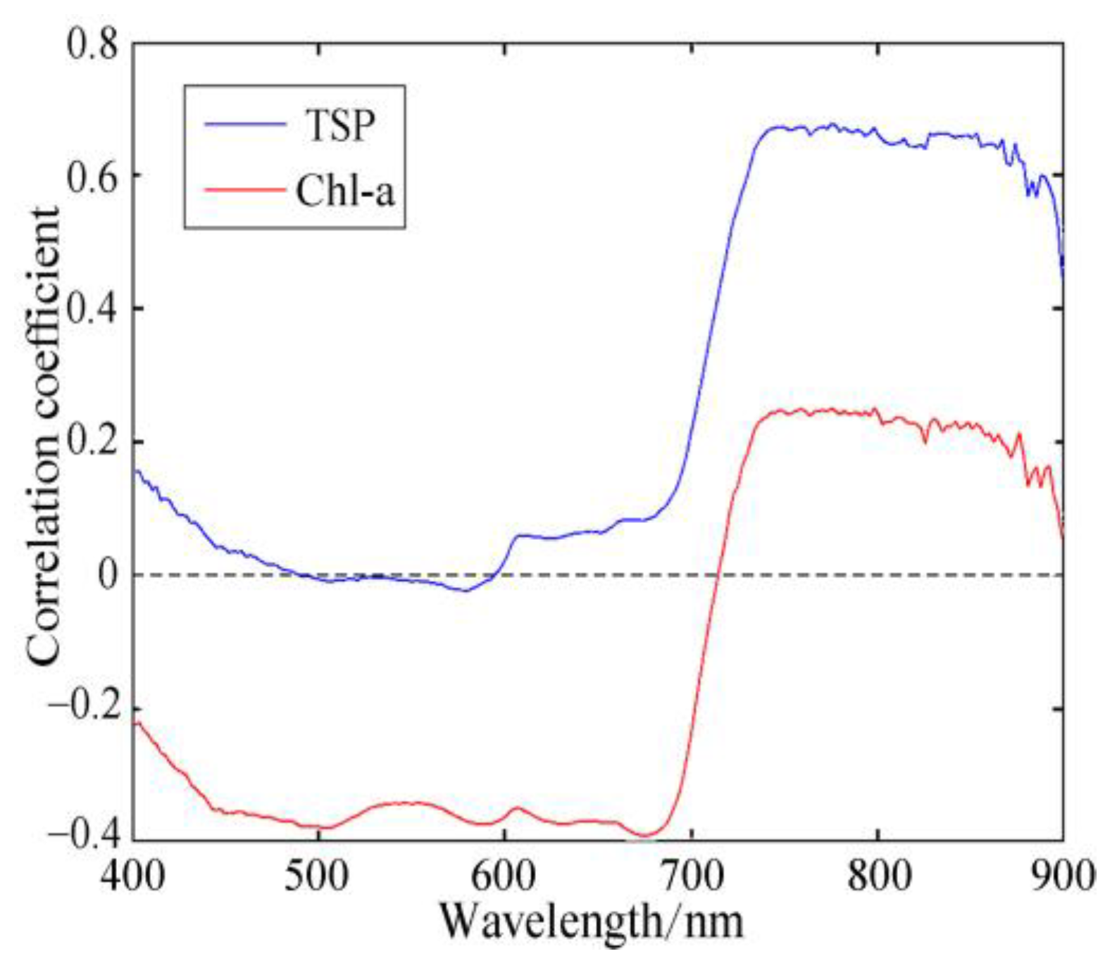
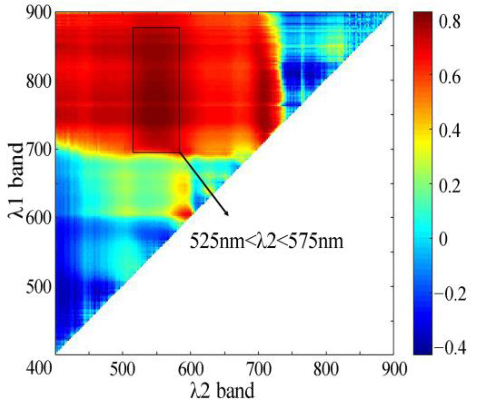
2.3.2. Retrieval Model of TSP

According to three different characteristic bands, empirical models and BPNN models were established to estimate the TSP concentrations (

Table 2. The total suspended particulate (TSP) retrieval models and the bands.

Model	Equation	Band
Two-band	${\mathrm{R}}_{\lambda 1}/{\mathrm{R}}_{\lambda 2}$ $\mathrm{B}\mathrm{P}\mathrm{N}\mathrm{N}\left({\lambda }_1,{\lambda }_2\right)$	${\lambda }_1$ = 670 nm or 750 nm or 850 nm, ${\lambda }_2$ = 555 nm
Three-band	$10ˆ[\mathrm{a}+\mathrm{b}({\mathrm{R}}_{\lambda 2}^{\mathrm{N}}+{\mathrm{R}}_{\lambda 3}^{\mathrm{N}})+\mathrm{c}({\mathrm{R}}_{\lambda 1}^{\mathrm{N}}/{\mathrm{R}}_{\lambda 2}^{\mathrm{N}}\left)\right]$ $\mathrm{B}\mathrm{P}\mathrm{N}\mathrm{N}({\lambda }_1,{\lambda }_2,{\lambda }_3)$	${\lambda }_1$ = 490 nm, ${\lambda }_2$ = 555 nm ${\lambda }_3$ = 670 nm

). The two-band ratio models have been widely used to retrieve TSP concentration [25,26,27]. Considering the wide range of TSP concentration in the study area, the ratios of 670, 750 and 850 to 555 nm were selected to establish the ratio models. The three-band statistical model was developed based on the ratio model by Tassan [28], which showed good performance in the retrieval of TSP concentration in different cases [29,30]. The BPNN models had four input forms, i.e., the bands in the four above-mentioned empirical statistical models were used as input variables. The optimal number of the hidden layer neurons was 3, and the other parameters of the BPNN models were the same as the BPNN models for Chl-a in the above section.

2.4. Model Training and Accuracy Verification

From 135 samples, 90 samples were randomly selected for model training, and 45 samples were used for model validation. The ten-fold cross-validation method was used for the BPNN model training. Statistics of water quality parameters for the training and validation samples are shown in

Table 3. Descriptions of the water quality characteristics.

Parameter	Dataset	Minimum	Maximum	Average	Standard Deviation
Chl-a (µg·L−1)	Training set	3	258	38.53	40.92
	Validation set	3	202	39.80	41.30
TSP (mg·L−1)	Training set	8	162	42.39	28.54
	Validation set	11	162	42.84	28.83

. Decision coefficient (R²), root mean square error (RMSE) and mean relative error (MRE) were used to evaluate the model.

3. Results and Analysis

3.1. Retrieval Results of the Chl-a Concentration

3.1.1. Two-Band Ratio Models

Five models (logarithmic model, linear model, exponential model, power model and quadratic polynomial model) were established on the basis of regression between Chl-a concentration and the ratio of reflectance at 705 and 670 nm. Furthermore, a BPNN model with the same two bands as input variables was set up for comparison (

Table 4. The two-band (R670, R705) models for Chl-a concentration.

Input	Regression Model	Equation	R2	RMSE (µg·L−1)	MRE (%)
	Logarithmic	Y = 156.19ln(x) + 2.03	0.62	29.90	89.44
	Linear	Y = 111.43x − 106.7	0.70	26.93	63.06
R705/R670	Exponential	$\mathrm{y}={1.28\mathrm{e}}^{2.26\mathrm{x}}$	0.73	71.99	43.93
	Power	$\mathrm{y}={10.66\mathrm{x}}^{3.51}$	0.81	34.40	34.13
	Quadratic polynomial	$\mathrm{y}=36.99{\mathrm{x}}^2-16.19\mathrm{x}-11.5$	0.81	21.52	27.93
R670, R705	BPNN	--	0.86	18.18	28.26

). In the ratio (R705/R670) models, the retrieval errors with the samples with high concentrations (>100 µg·L⁻¹) were large, which led to a high RMSE. The linear model brought more negative values in the low-concentration samples (<10 µg·L⁻¹), and the MRE was large. Among the five regression models, the retrieval accuracy of the logarithmic model was the lowest, and the quadratic polynomial model had the highest accuracy.

Compared with the quadratic polynomial model, the MRE of the BPNN model increased from 27.93% to 28.26% and the R² value increased from 0.81 to 0.86, while the RMSE decreased from 21.52 to 18.18 µg·L⁻¹. This indicates that the BPNN model can also produce satisfactory retrieval results.

3.1.2. T-Depth Models

There was a positive exponential relationship with “e” natural base between Chl-a concentration and the T-depth index (

Table 5. The T-depth and back-propagation neural network (BPNN) (R650, R675, R700) models for Chl-a concentration.

Input	Equation	R2	RMSE (µg·L−1)	MRE (%)
T-depth (${\mathrm{R}}_{\lambda \mathrm{i}}$)	$\mathrm{y}={8.71\mathrm{e}}^{219.54\mathrm{x}}$	0.39	45.01	60.59
T-depth (${\mathrm{R}}_{\lambda \mathrm{i}}^{\mathrm{N}}$)	$\mathrm{y}={6.41\mathrm{e}}^{4.62\mathrm{x}}$	0.61	39.36	44.72
R650, R675, R700	BPNN	0.83	20.40	28.01

), which is consistent with the results of Xing et al. [22]. The modeling results show that the T-depth statistical model calculated by a normalized spectrum can improve the retrieval accuracy, but the error is still large. Meanwhile, the BPNN model with characteristic bands from the T-depth index as input has better results (R² = 0.83, RMSE = 20.4 µg·L⁻¹, MRE = 28.01%). This case suggests that the machine learning approach of BPNN has the advantage in modeling in a non-linear way under certain conditions.

3.1.3. Three-Band Models

There was a significant linear relationship between Chl-a concentration and three-band models (

Table 6. The three-band (R670, R710, R750) models for Chl-a concentration.

Input	Equation	R2	RMSE (µg·L−1)	MRE (%)
${\mathrm{R}}_{670}^{-1}-{\mathrm{R}}_{710}^{-1}$	Y = 158.07x + 15	0.89	17.18	25.41
R670, R710, R750	BPNN	0.92	14.29	21.86

). Among the retrieval models tested in this paper, the three-band models had the highest retrieval accuracy. Compared with the three-band empirical model, the R² of three-band BPNN model increased by 3.4% from 0.89 to 0.92, the RMSE decreased from 17.18 to 14.29 µg·L⁻¹ and the MRE decreased by 16.8% from 25.41% to 21.86%.

3.1.4. Model Validation

The established models were further tested with the validation dataset, and the estimated Chl-a concentrations were compared with the measured values. The results show that the retrieval accuracies of each model with the training set and the validation set are close. For each band combination, the accuracies of BPNN models are usually improved when they are compared with the corresponding empirical statistical models. For the three-band model with a higher accuracy, the model also had a satisfactory retrieval result on the validation set (Figure 3g,h); compared with the three-band statistical model, the BPNN model slightly improved the retrieval accuracy with R² increasing from 0.85 to 0.92, and with the MRE decreasing from 25.88% to 22.56%. The retrieval accuracy of the two-band BPNN model was improved, although in a small magnitude (Figure 3a,b). The validation results of the T-depth model are close to the training results (Figure 3d); however, the validation accuracy of the BPNN model was significantly improved (Figure 3e), which was consistent with the training set. The relative error distributions of the BPNN model and the corresponding empirical statistical model are shown in Figure 3c,f,i; the results show that the model with higher accuracy tends to present an error distribution with higher frequency at the middle and lower at two sides and that the error distribution of the three-band combination is close to a normal distribution with more bias values lower than 30%.

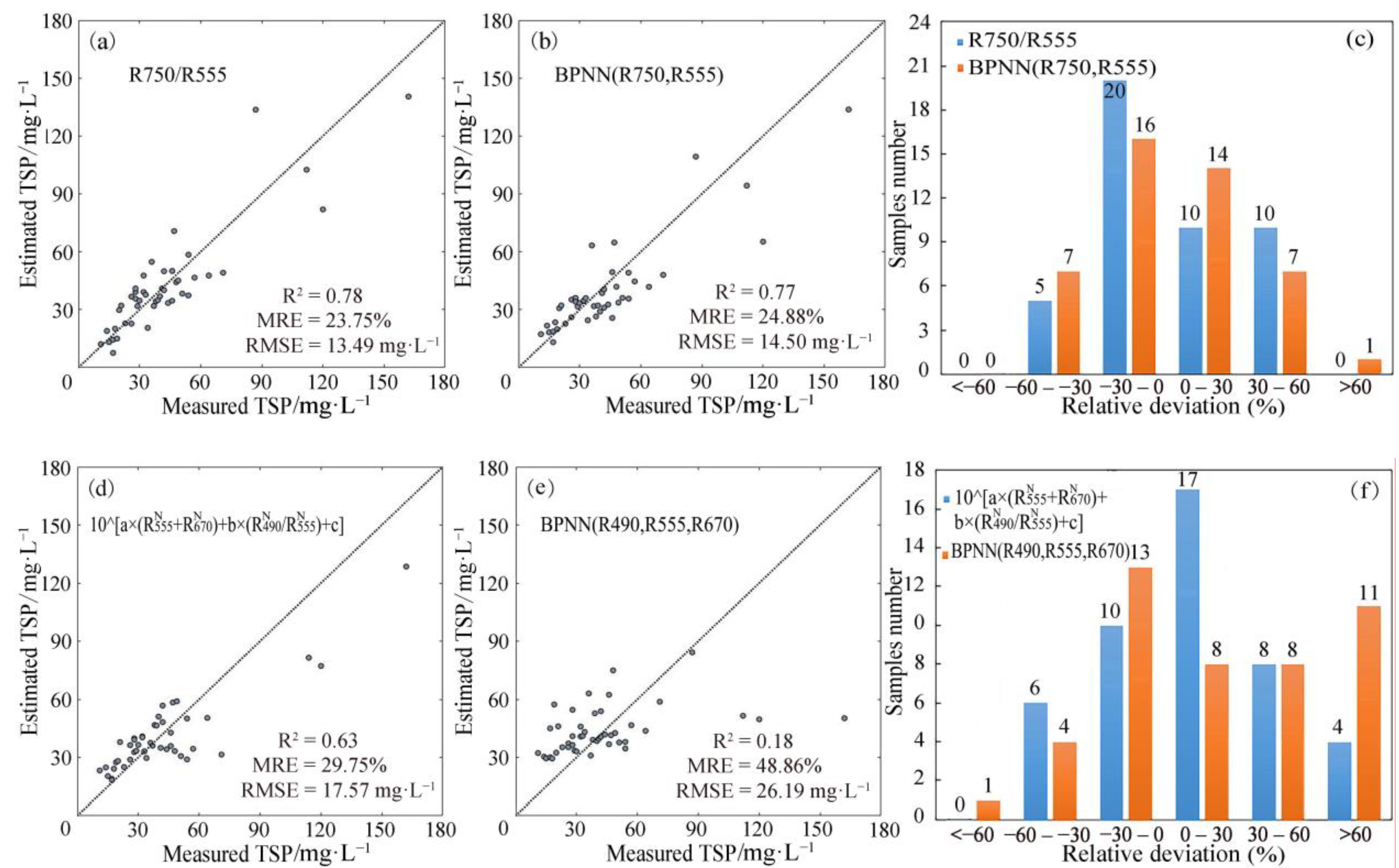
3.2. Retrieval Results of TSP Concentration

3.2.1. Two-Band Ratio Models

On the basis of the linear relationships between different band ratio combinations and the TSP concentration, three models were established (

Table 7. The two-band (R555, R670), (R555, R750) or (R555, R850) models for TSP concentration.

Input	Equation	R2	RMSE (mg·L−1)	MRE (%)
R670/R555	Y = 42.14x + 7.16	0.07	27.54	58.44
R750/R555	Y = 101.9x − 1.44	0.74	14.81	23.05
R850/R555	Y = 116.43x	0.67	17.09	28.10
R555, R670	BPNN	0.12	28.43	45.48
R555, R750	BPNN	0.76	14.99	23.91
R555, R850	BPNN	0.68	16.33	27.89

). The results show that the near infrared–green band ratio models (R750/R555, R850/R555) have better retrieval performances and that the model of R750/R555 has the highest retrieval accuracy, with R² up to 0.74. The retrieval accuracy of the red–green band ratio model (R670/R555) for TSP is low, with R² of 0.07. The retrieval accuracies of the BPNN model and the empirical model with the combination of (R555, R750) or (R555, R850) are very close to each other.

3.2.2. Three-Band Models

There was a positive exponential relationship between the TSP concentration and three-band combinations (

Table 8. The three-band (R490, R555, R670) models for TSP concentration.

Input	Equation	R2	RMSE (mg·L−1)	MRE (%)
$\mathrm{x}1:\mathrm{R}555+\mathrm{R}670$ $\mathrm{x}1:\mathrm{R}490/\mathrm{R}555$	$\mathrm{y}={10}^{1.38+1.07\mathrm{x}1+0.2\mathrm{x}2}$	0.01	29.19	48.10
$\mathrm{x}1:{\mathrm{R}}_{555}^{\mathrm{N}}+{\mathrm{R}}_{670}^{\mathrm{N}}$ $\mathrm{x}2:{\mathrm{R}}_{490}^{\mathrm{N}}+{\mathrm{R}}_{555}^{\mathrm{N}}$	$\mathrm{y}={10}^{2.89-0.48\mathrm{x}1+0.1\mathrm{x}2}$	0.42	21.89	32.60
R490, R555, R670	BPNN	0.25	24.09	49.09

), which is consistent with the research results of Siswanto et al. [29]. The results show that although the spectral normalization method can improve the retrieval accuracy of three-band statistical models, the accuracy is still not good, which may be due to the low correlation between the characteristic bands used in the statistical model and TSP concentration. In addition, the accuracy of the BPNN model with three bands as input was lower than that of the three-band statistical model.

3.2.3. Model Validation

The results of the validation test show that the retrieval accuracy of each model on the training set and the validation set is also close. Unlike the retrieval models for Chl-a, the BPNN models for TSP barely improve retrieval accuracy when they are compared with the corresponding empirical statistical models. For the two-band ratio model (R750/R555) with high accuracy (Figure 4a,b), the model also had satisfactory retrieval results with the validation set. Compared with the ratio model, the accuracy of the BPNN model with the two bands as input was almost unchanged. The validation result of the three-band model was close to the training results, and the statistical model did not reach satisfactory validation accuracy (Figure 4d,e); moreover, the BPNN model had lower retrieval accuracy than that of its corresponding empirical model. From the distribution in relative errors, it can be seen that the two-band combination had close to a normal distribution, with more bias values lower than 30% (Figure 4c). In the three-band combination, both the BPNN model and the empirical statistical model tended to overestimate the TSP concentration (Figure 4f).

4. Discussion

In this work, two types of models for monitoring the water optical substances (Chl-a and TSP), i.e., traditional empirical models and machine learning models of BPNN, are evaluated. The results show that the performance of the two types of retrieval models is highly affected by the changes in the input band settings. The results of correlation analysis between the Rrs and the two optically active substances of Chl-a and TSP are shown in Figure 5. Generally, the Rrs is highly correlated with the TSP concentration in the near-infrared spectral region, and the correlation coefficients are greater than 0.6. In the visible range, the Rrs and the Chl-a concentration tend to be negatively correlated, which is consistent with the absorptions of Chl-a, especially at 440 and 675 nm.

In this work, the three-band statistical model with high accuracy in Chl-a retrieval is compared with previous research (

Table 9. Comparison of retrieval results for three-band Chl-a models.

Model	Sample Number	TSP (mg·L−1)	Chl-a (µg·L−1)	R2
$({\mathrm{R}}_{684}^{-1}-{\mathrm{R}}_{690}^{-1})\times \mathrm{R}718$ (Chen et al., 2011 [31])	32	40.8	17.6	0.81
$({\mathrm{R}}_{671}^{-1}-{\mathrm{R}}_{710}^{-1})\times \mathrm{R}740$ (Dall’Olmo et al., 2005 [32])	86	18.9	46.50	0.94
$({\mathrm{R}}_{670}^{-1}-{\mathrm{R}}_{710}^{-1})\times \mathrm{R}750$ (this paper)	90	42.39	38.53	0.89

). The water samples collected by Chen et al. [31] had low Chl-a concentration and high TSP concentration, indicating that the portion of algae particles in the TSP content was low. On the contrary, the water samples collected by Dall’Olmo et al. [32] had high Chl-a concentration and low TSP concentration, indicating a high portion of algae particles in TSP, and the retrieval accuracy of the model for Chl-a was high. Previous studies have shown that when the concentration of algae particles in water is high, there is a strong spectral signal of Chl-a, and the retrieval accuracy is usually high [33]. Water samples in this work had both high Chl-a concentration and high TSP concentration, indicating that the water is dominated by algae particles and non-algae particles.

In a similar way, the two-band ratio model (R750/R555) for TSP was compared with previous work (

Table 10. Comparison of retrieval results for two-band TSP ratio models.

Model	Sample Number	TSP (mg·L−1)	Chl-a (µg·L−1)	R2
R700/R670 (Matthews et al., 2010 [34])	31	49.1	148.6	0.66
R645/R858 (Wang et al., 2012 [36])	35	705	1.16	0.82
R750/R555 (This paper)	90	42.39	38.53	0.74

). For the denominator in the ratio model, the green band was better than the red band in previous models (Figure 6). In the water samples collected by Matthews et al. [34], the portion of non-algae particles was low in the TSP content, and the model accuracy was relatively low. When Chl-a concentration is low, the absorption of total suspended particulate shows an absorption spectral pattern of non-algal particles [35]. The ratio model established by Wang et al. [36] had high retrieval accuracy, which is consistent with the high proportion of non-algae particles.

As discussed above, the training datasets corresponding to various water quality conditions highly affect the performance of retrieval models. For example, in this work, samples with high values (Chl-a > 100 µg·L⁻¹, TSP > 70 mg·L⁻¹) are relatively few, which may lead to uncertainty in the retrieval accuracy when the models are applied to extremely turbid and eutrophic waters. Especially for the machine learning approaches without considering the characteristic bands of water quality parameters, a large dataset covering wide water conditions is necessary.

5. Summary

Analysis with the in situ collected water samples showed that the water body in the Pearl River Delta is characterized by high Chl-a concentration (3 to 256 µg·L⁻¹) and high TSP concentration (8 to 162 mg·L⁻¹). In this work, traditional empirical models and BPNN models with corresponding spectral bands were established to monitor the concentrations of Chl-a and TSP, and the models’ performances were evaluated. For the two optically active substances of Chl-a and TSP, both traditional empirical models and BPNN models work well to estimate their concentrations, although the accuracies of these models are highly dependent on the band selections. Optimized band selections can significantly improve models’ accuracies, and the corresponding BPNN models, on the basis of the characteristic bands used in the empirical models, may generally improve the retrieval accuracies. However, the BPNN models are not always better than the traditional models, e.g., in the estimation of TSP.

Considering that sufficient and representative samples are necessary for training BPNN models, the modeling cost is usually higher than that of empirical models. Although there were 135 sets of data in this study, the lowest values of Chl-a and TSP concentrations in this work are 3 and 8 mg·L⁻¹, respectively, which means that a water body with Chl-a and TSP lower than the lowest values may not be monitored on the basis of the BPNN models. A hyperspectral reflectance sensor network is a good approach for monitoring water quality in a green way. To improve the performance of machine learning models in future applications on the basis of a ground reflectance sensor network, large datasets covering various water situations and optimization of the input variable of band configuration are still necessary.

References

1. Xing, Q.G.; Lou, M.J.; Chen, C.Q.; Shi, P. Using in situ and satellite hyperspectral data to estimate the surface suspended sediments concentrations in the Pearl River Estuary. IEEE J. Sel. Top. Appl. Earth Observ. Remote Sens. 2013, 6, 731–738. [Google Scholar] [CrossRef]
2. Liu, F.F.; Tang, S.L. Evaluation of red-peak algorithms for chlorophyll measurement in the Pearl River Estuary. IEEE Trans. Geosci. Remote Sens. 2019, 57, 8928–8936. [Google Scholar] [CrossRef]
3. Li, J.; Chen, X.L.; Tian, L.Q.; Huang, J.; Feng, L. Improved capabilities of the Chinese high-resolution remote sensing satellite GF-1 for monitoring suspended particulate matter (SPM) in inland waters: Radiometric and spatial considerations. ISPRS-J. Photogramm. Remote Sens. 2015, 106, 145–156. [Google Scholar] [CrossRef]
4. Wang, X.; Gong, Z.N.; Pu, R.L. Estimation of chlorophyll a content in inland turbidity waters using WorldView-2 imagery: A case study of the Guanting Reservoir, Beijing, China. Environ. Monit. Assess. 2018, 190, 620. [Google Scholar] [CrossRef]
5. Tang, S.L.; Larouche, P.; Niemi, A.; Michel, C. Regional algorithms for remote-sensing estimates of total suspended matter in the Beaufort Sea. Int. J. Remote Sens. 2013, 34, 6562–6576. [Google Scholar] [CrossRef]
6. Gurlin, D.; Gitelson, A.A.; Moses, W.J. Remote estimation of Chl-a concentration in turbid productive waters—Return to a simple two-band NIR-red model? Remote Sens. Environ. 2011, 115, 3479–3490. [Google Scholar] [CrossRef]
7. Zhang, M.W.; Tang, J.W.; Dong, Q.; Song, Q.T.; Ding, J. Retrieval of total suspended matter concentration in the Yellow and East China Seas from MODIS imagery. Remote Sens. Environ. 2010, 114, 392–403. [Google Scholar] [CrossRef]
8. Li, J.S.; Gao, M.; Feng, L.; Zhao, H.L.; Shen, Q.; Zhang, F.F.; Wang, S.L.; Zhang, B. Estimation of chlorophyll-a concentration in a highly turbid eutrophic lake using a classification-based MODIS land-band algorithm. IEEE J. Sel. Top. Appl. Earth Observ. Remote Sens. 2019, 12, 3769–3783. [Google Scholar] [CrossRef]
9. Zhang, F.F.; Li, J.S.; Shen, Q.; Zhang, B.; Wu, C.Q.; Wu, Y.F.; Wang, G.L.; Wang, S.L.; Lu, Z.Y. Algorithms and schemes for chlorophyll a estimation by remote sensing and optical classification for turbid lake Taihu, China. IEEE J. Sel. Top. Appl. Earth Observ. Remote Sens. 2015, 8, 350–364. [Google Scholar] [CrossRef]
10. Guo, H.W.; Huang, J.H.; Chen, B.W.; Guo, X.L.; Singh, V.P. A machine learning-based strategy for estimating non-optically active water quality parameters using Sentinel-2 imagery. Int. J. Remote Sens. 2020, 42, 1841–1866. [Google Scholar] [CrossRef]
11. Kuan, H.F.; Li, J.; Zhang, X.J.; Zhang, J.P.; Cui, H.; Sun, Q. Remote estimation of water quality parameters of medium- and small-sized inland rivers using Sentinel-2 imagery. Water 2020, 12, 3124. [Google Scholar]
12. Saberioon, M.; Brom, J.; Nedbal, V.; Soucek, P.; Cisar, P. Chlorophyll-a and total suspended solids retrieval and mapping using Sentinel-2A and machine learning for inland waters. Ecol. Indic. 2020, 113, 106236. [Google Scholar] [CrossRef]
13. Nazeer, M.; Bilal, M.; Alsahli, M.M.; Shahzad, M.I.; Waqas, A. Evaluation of empirical and machine learning algorithms for estimation of coastal water quality parameters. ISPRS. Int. J. Geo-Inf. 2017, 6, 360. [Google Scholar] [CrossRef] [Green Version]
14. Ioannou, I.; Gilerson, A.; Gross, B.; Moshary, F.; Ahmed, S. Deriving ocean color products using neural networks. Remote Sens. Environ. 2011, 134, 78–91. [Google Scholar] [CrossRef]
15. Kim, T.H.; Kim, Y.W.; Shin, H.; Go, B.G.; Cha, Y.K. Assessing land-cover effects on stream water quality in metropolitan areas using the water quality index. Water 2020, 12, 3294. [Google Scholar] [CrossRef]
16. Cai, J.N.; Liu, H.L.; Jiang, B.; He, T.H.; Chen, W.J.; Feng, Z.W.; Li, Z.L.; Xing, Q.G. Using hyperspectral imagery and GA-PLS algorithm to estimate chemical oxygen demand concentration of waters is river network. J. Irrig. Drain. 2020, 39, 126–131. [Google Scholar]
17. Wang, J.L.; Fu, Z.S.; Qiao, H.X.; Liu, F.X. Assessment of eutrophication and water quality in the estuarine area of Lake Wuli, Lake Taihu, China. Sci. Total Environ. 2019, 650, 1392–1402. [Google Scholar] [CrossRef] [PubMed]
18. Wu, C.Y.; Ren, J.; Bao, Y.; Shi, H.Y.; Lei, Y.P.; He, Z.G.; Tang, Z.M. A preliminary study on the morphodynamic evolution of the ‘gate’ of the Pearl River Delta, China. Acta Geogr. Sin. 2006, 5, 537–548. [Google Scholar]
19. Tang, J.W.; Tian, G.L.; Wang, X.Y.; Wang, X.M.; Song, Q.J. The methods of water spectra measurement and analysis I: Above-water method. J. Remote Sens. 2004, 8, 37–44. [Google Scholar]
20. Le, C.; Hu, C.; Cannizzaro, J.; English, D.; Muller-Karger, F.; Lee, Z. Evaluation of chlorophyll-a remote sensing algorithms for an optically complex estuary. Remote Sens. Environ. 2013, 129, 75–89. [Google Scholar] [CrossRef]
21. Gons, H.J. Optical teledetection of chlorophyll a in turbid inland waters. Environ. Sci. Technol. 1999, 33, 1127–1132. [Google Scholar] [CrossRef]
22. Xing, Q.G.; Yu, D.F.; Lou, M.J.; Lv, Y.C.; Li, S.P.; Han, Q.Y. Using in-situ reflectance to monitor the chlorophyll concentration in the surface layer of tidal flat. Spectrosc. Spectr. Anal. 2013, 33, 2188–2191. [Google Scholar]
23. Gitelson, A.A.; Dall’Olmo, G.; Moses, W. A simple semi-analytical model for remote estimation of chlorophyll-a in turbid waters: Validation. Remote Sens. Environ. 2008, 112, 3582–3593. [Google Scholar] [CrossRef]
24. Shen, C.Y.; Chen, C.Q.; Zhan, H.G. Inverse of chlorophyll concentration in Zhujiang River estuary using artificial neural network. J. Trop. Oceanogr. 2005, 24, 38–43. [Google Scholar]
25. Doxaran, D.; Froidefond, J.M.; Castaing, P. Remote-sensing reflectance of turbid sediment-dominated waters. Reduction of sediment type variations and changing illumination conditions effects by use of reflectance ratios. Appl. Opt. 2003, 42, 2623–2634. [Google Scholar] [CrossRef] [PubMed]
26. Tian, L.Q.; Wai, O.W.H.; Chen, X.L.; Li, W.B.; Li, J.; Li, W.K.; Zhang, H.D. Retrieval of total suspended matter concentration from Gaofen-1 Wide Field Imager (WFI) multispectral imagery with the assistance of Terra MODIS in turbid water–case in Deep Bay. Int. J. Remote Sens. 2016, 37, 3400–3413. [Google Scholar] [CrossRef]
27. Li, J.; Tian, L.Q.; Song, Q.J.; Huang, J.; Li, W.K.; Wei, A.N. A near-infrared band-based algorithm for suspended sediment estimation for turbid waters using the experimental Tiangong 2 moderate resolution wide-wavelength imager. IEEE J. Sel. Top. Appl. Earth Observ. Remote Sens. 2019, 12, 774–787. [Google Scholar] [CrossRef]
28. Tassan, S. Local algorithms using SeaWiFS data for the retrieval of phytoplankton, pigments, suspended sediment, and yellow substance in coastal waters. Appl. Opt. 1994, 33, 2369–2378. [Google Scholar] [CrossRef]
29. Siswanto, E.; Tang, J.W.; Yamaguchi, H.; Ahn, Y.H.; Ishizaka, J.; Yoo, S.; Kim, S.W.; Kiyomoto, Y.; Yamada, K.; Chiang, C.; et al. Empirical ocean-color algorithms to retrieve chlorophyll-a, total suspended matter, and colored dissolved organic matter absorption coefficient in the Yellow and East Chinese Seas. J. Oceanogr. 2011, 67, 627–650. [Google Scholar] [CrossRef]
30. Han, B.; Loisel, H.; Vantrepotte, V.; Mériaux, X.; Bryère, P.; Ouillon, S.; Dessailly, D.; Xing, Q.G.; Zhu, J.H. Development of a semi-analytical algorithm for the retrieval of suspended particulate matter from remote sensing over clear to very turbid waters. Remote Sens. 2016, 8, 211. [Google Scholar] [CrossRef] [Green Version]
31. Chen, S.S.; Fang, L.G.; Li, H.L.; Chen, W.Q.; Huang, W.R. Evaluation of a three-band model for estimating chlorophyll-a concentration in tidal reaches of the Pearl River Estuary, China. ISPRS-J. Photogramm. Remote Sens. 2011, 66, 356–364. [Google Scholar] [CrossRef]
32. Dall’Olmo, G.; Gitelson, A.A. Effect of bio-optical parameter variability on the remote estimation of chlorophyll-a concentration in turbid productive waters: Experimental results. Appl. Opt. 2005, 44, 412–422. [Google Scholar] [CrossRef] [Green Version]
33. Zhang, Y.L.; Feng, S.; Ma, R.H.; Liu, M.L. Spatial variation and estimation of optically active substances in Taihu lake in Autumn of 2004. Geomat. Inf. Sci. Wuhan Univ. 2008, 33, 967–972. [Google Scholar]
34. Matthews, M.W.; Bernard, S.; Winter, K. Remote sensing of cyanobacteria-dominant algal blooms and water quality parameters in Zeekoevlei, a small hypertrophic lake, using MERIS. Remote Sens. Environ. 2010, 114, 2070–2087. [Google Scholar] [CrossRef]
35. Wang, M.Z.; Zhang, Y.L.; Shi, K.; Gao, Y.; Liu, G.; Jiang, H. Characteristics of optical absorption coefficients and their differences in typical seasons in lake Qiandaohu. Environ. Sci. 2014, 35, 2528–2538. [Google Scholar]
36. Wang, F.; Zhou, B.; Liu, X.M.; Zhou, G.D.; Zhao, K.L. Remote-sensing inversion model of surface water suspended sediment concentration based on in situ measured spectrum in Hangzhou Bay, China. Environ. Earth Sci. 2012, 67, 1669–1677. [Google Scholar] [CrossRef]
Figure 1. (a) Location of the study area; (b) drainage distribution in the study area; (c) field photos of some typical sampling points ((c1c4), corresponding to the sampling point numbers in (b).
Water 13 00650 g001
Figure 2. Spectral reflectance. (a) The training samples (N = 90) and (b) the validation samples (N = 45).
Water 13 00650 g002
Figure 3. Scatter plot (the dotted line is the 1:1 line) for (a) The ratio model (R705/R670), (b) The BPNN model (R705, R670), (d) The t-depth statistical model, (e) The BPNN model (R650, R675, R700), (g) The three-band statistical model and (h) The BPNN model (R670, R710, R750), and relative deviation distribution between the measured values and retrieval values for (c) The two-band combination models, (f) The T-depth statistical model and corresponding BPNN model and (i) The three-band combination models for chlorophyll-a (Chl-a) concentration.
Water 13 00650 g003aWater 13 00650 g003b
Figure 4. Scatter plot (the dotted line is the 1:1 line) for (a) The ratio model (R750/R555), (b) The BPNN model (R705, R670), (d) The three-band statistical model, (e) The BPNN model (R490, R555, R670) and relative deviation distribution between measured values and retrieval values for (c) The two-band combination models, (f) The three-band combination models for total suspended particulate (TSP) concentration.
Water 13 00650 g004
Figure 5. Correlation coefficient between remote sensing reflectance and TSP/Chl-a concentration.
Water 13 00650 g005
Figure 6. Correlation coefficient matrix between TSP concentration and reflectance ratio combination (high-value area of correlation is enclosed by a black box).
Water 13 00650 g006