
A Planning Tool for Optimizing Investment to Reduce Drinking Water Risk to Multiple Water Treatment Plants in Open Catchments

Abstract
:1. Introduction
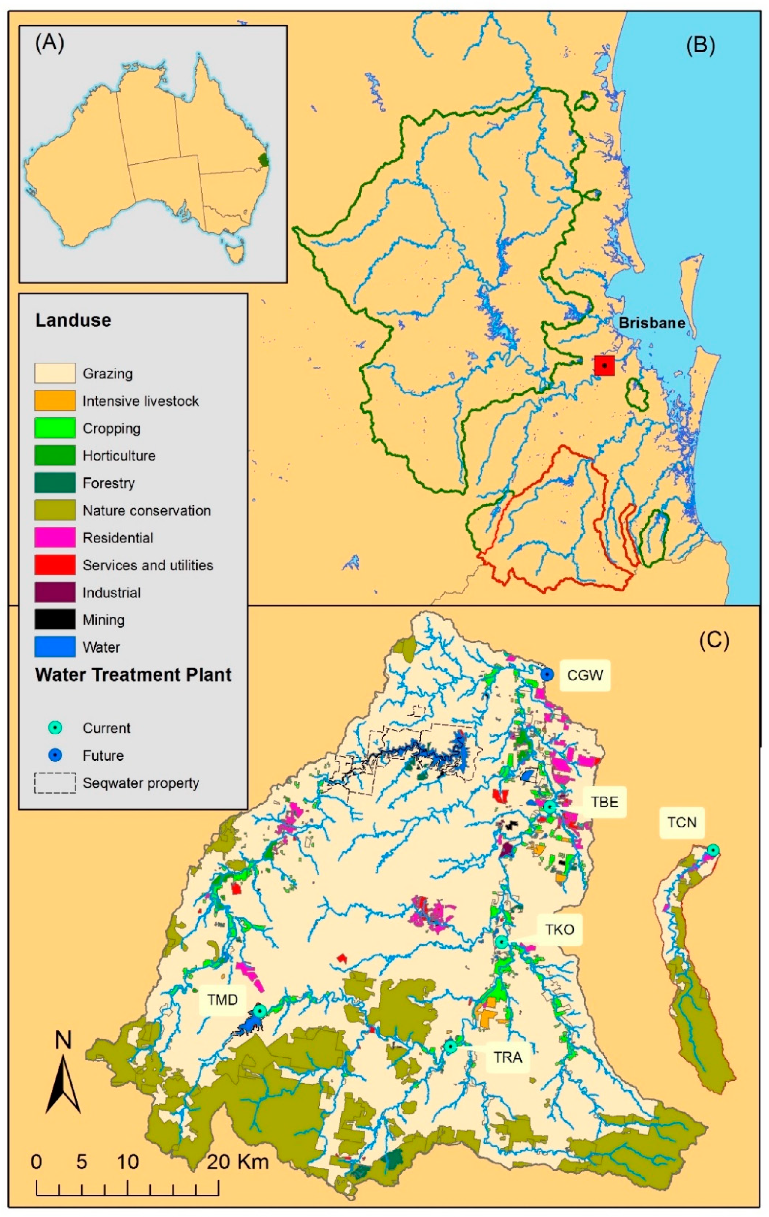
2. Study Area
3. Materials and Methods
3.1. Catchment Investment Decision Support System
3.1.1. Inputs
3.1.2. Computational Steps
Data Preparation
Risk at Plant Conversion
Optimisation Function
- Randomly move or alter the state.
- Assess the energy of the new state using an objective function.
- Compare the energy to the previous state and decide whether to accept the new solution or reject it based on the current temperature.
- Repeat until you have converged on an acceptable answer.
- The scenario causes a decrease in state energy (i.e., an improvement in the objective function), or
- The scenario increases the state energy (i.e., a slightly worse solution) but is within the bounds of the temperature. The temperature exponentially decreases as the algorithm progresses. In this way, we avoid getting trapped by local minima early in the process but start to hone a viable solution by the end.
- Tmax—the maximum starting temperature.
- Tmin—the ending temperature.
- Steps—the number of iterations in the simulation.
- Max_saturated_Steps—the maximum number of iterations to consider from a point determined to be close to a solution.
3.1.3. Interpreting Results
3.2. Scenario Case Study
4. Results and Discussion
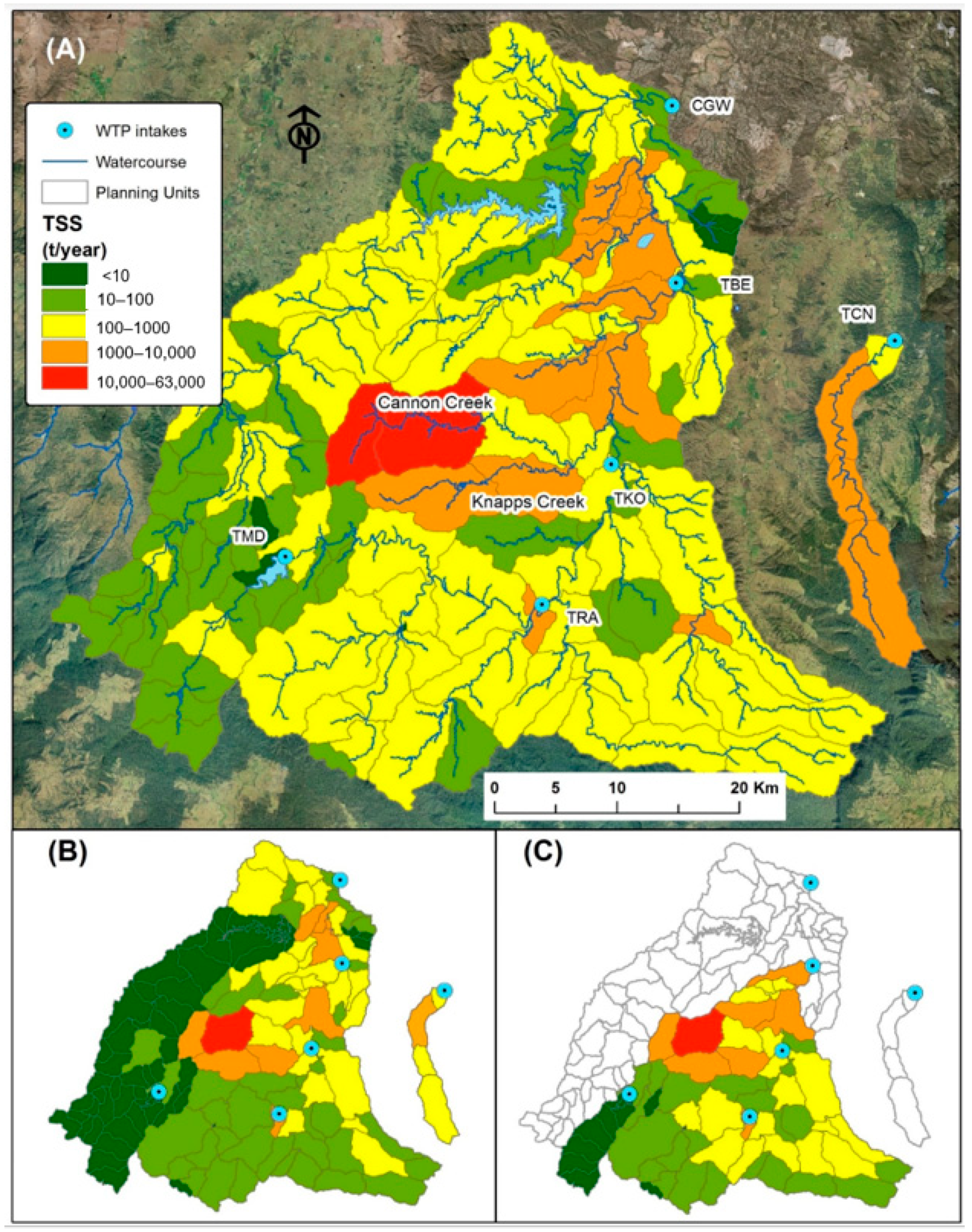
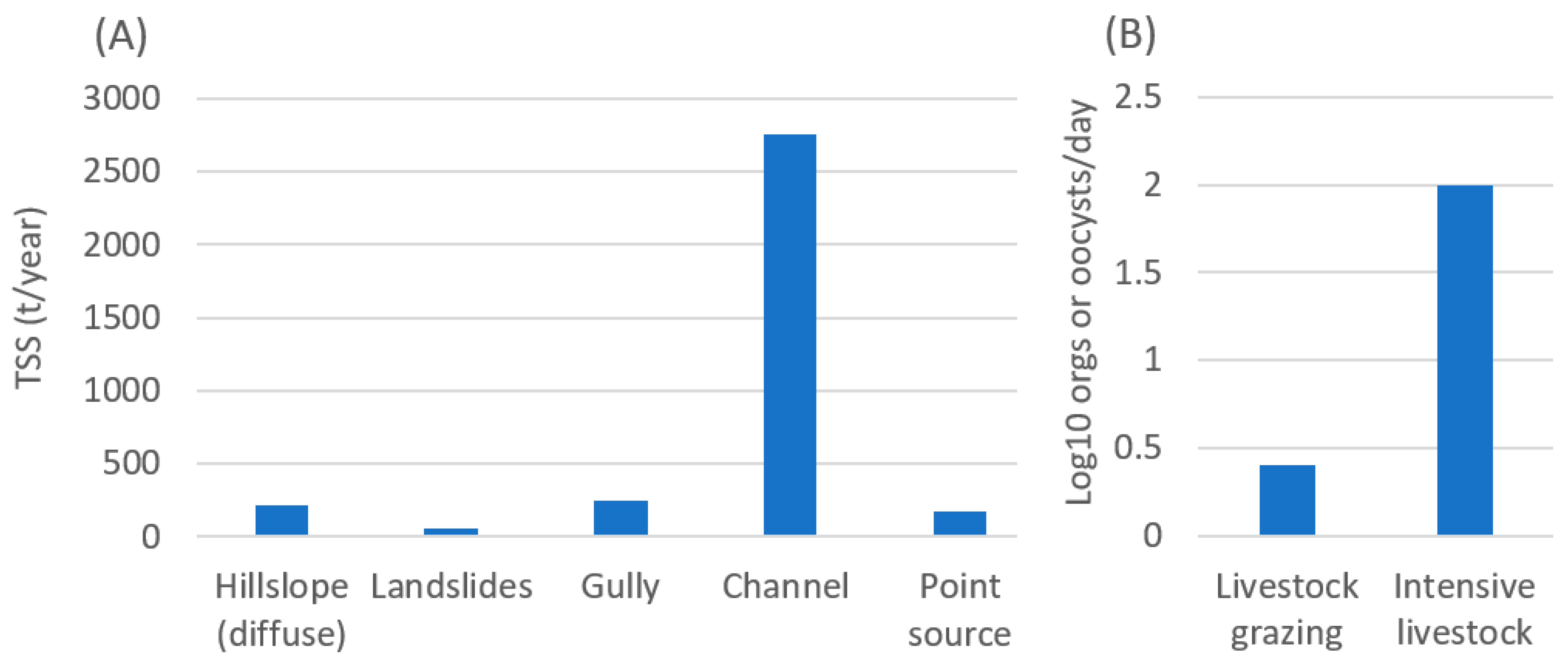
4.1. Current State of Source Catchment Water Quality
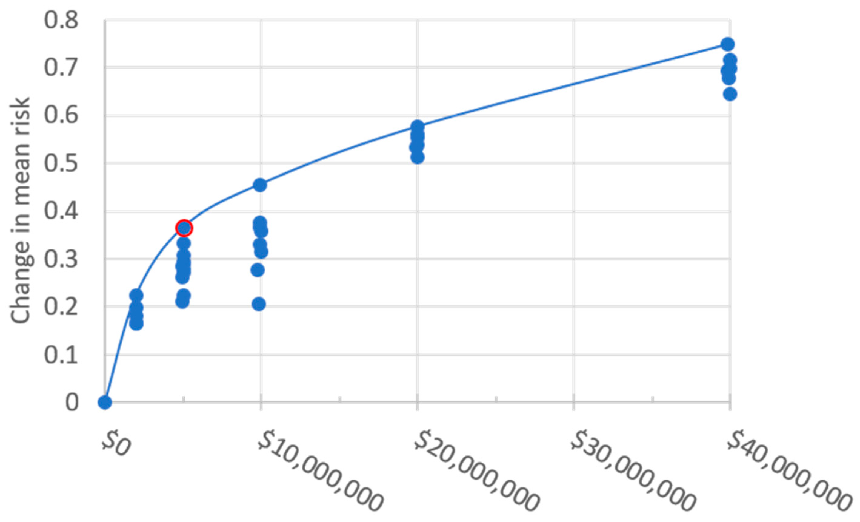
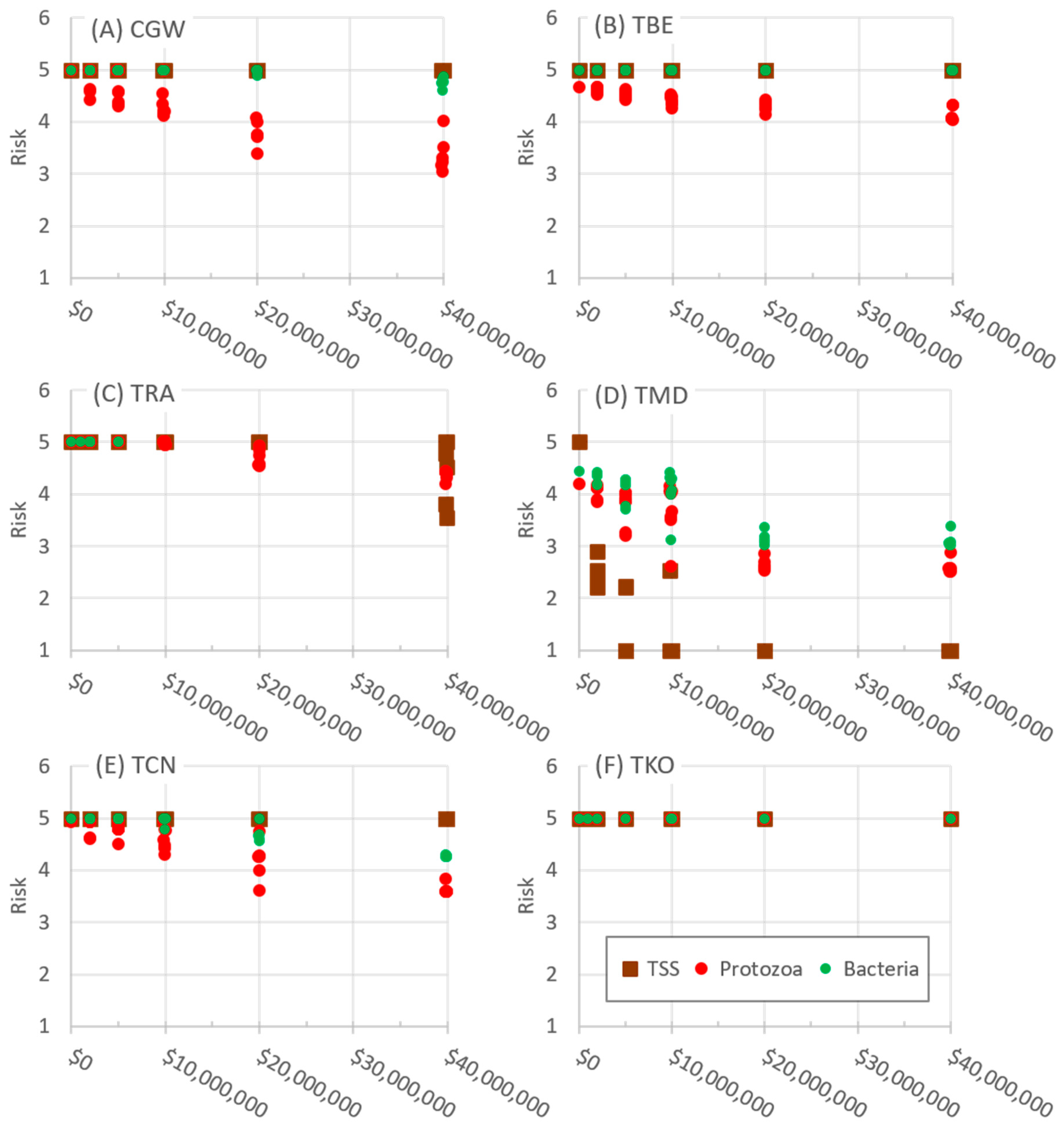
4.2. Potential for Source Water Risk Reduction
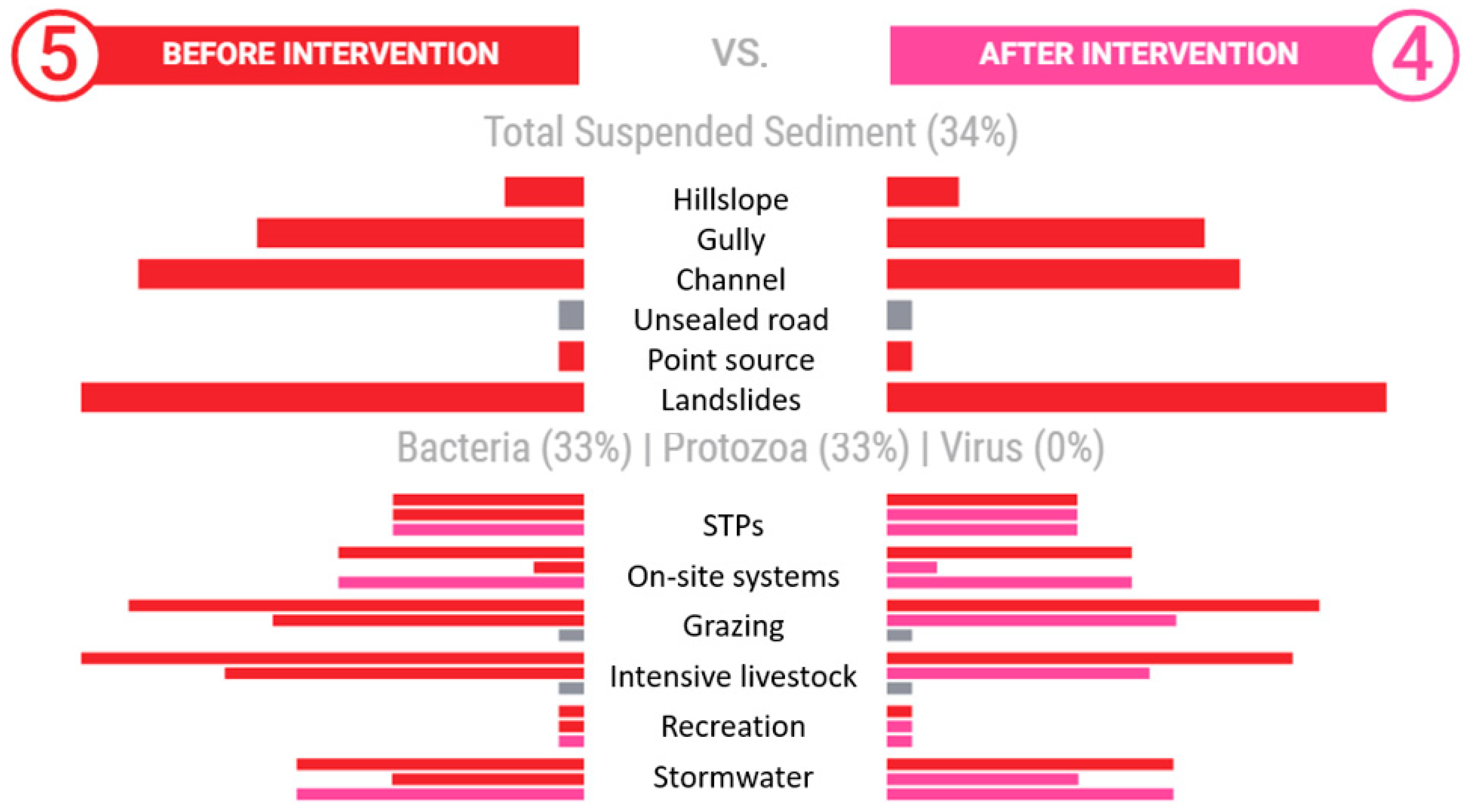
4.3. Selected Scenario
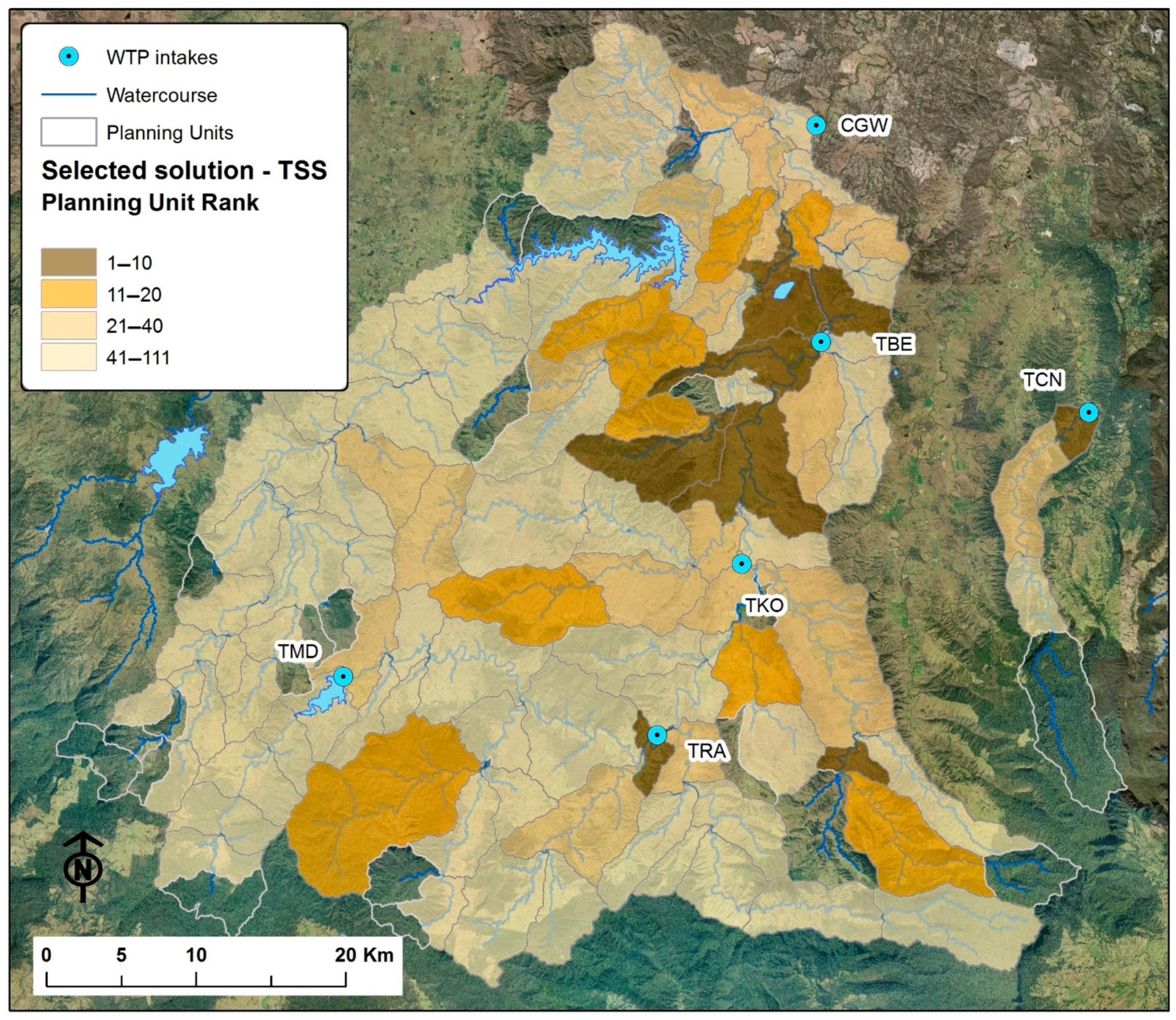
4.4. Prioritisation of CIDSS Solution
4.5. Consequence of Increasing Water Supply in Open Catchments
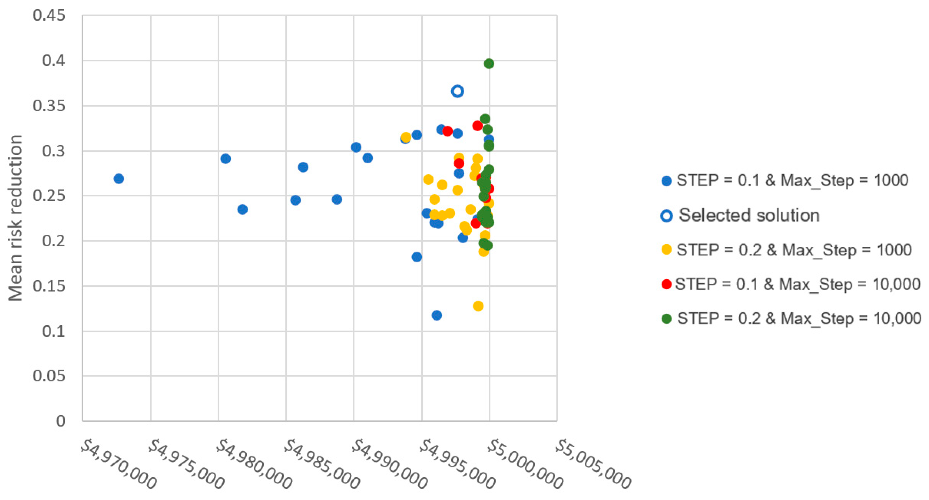
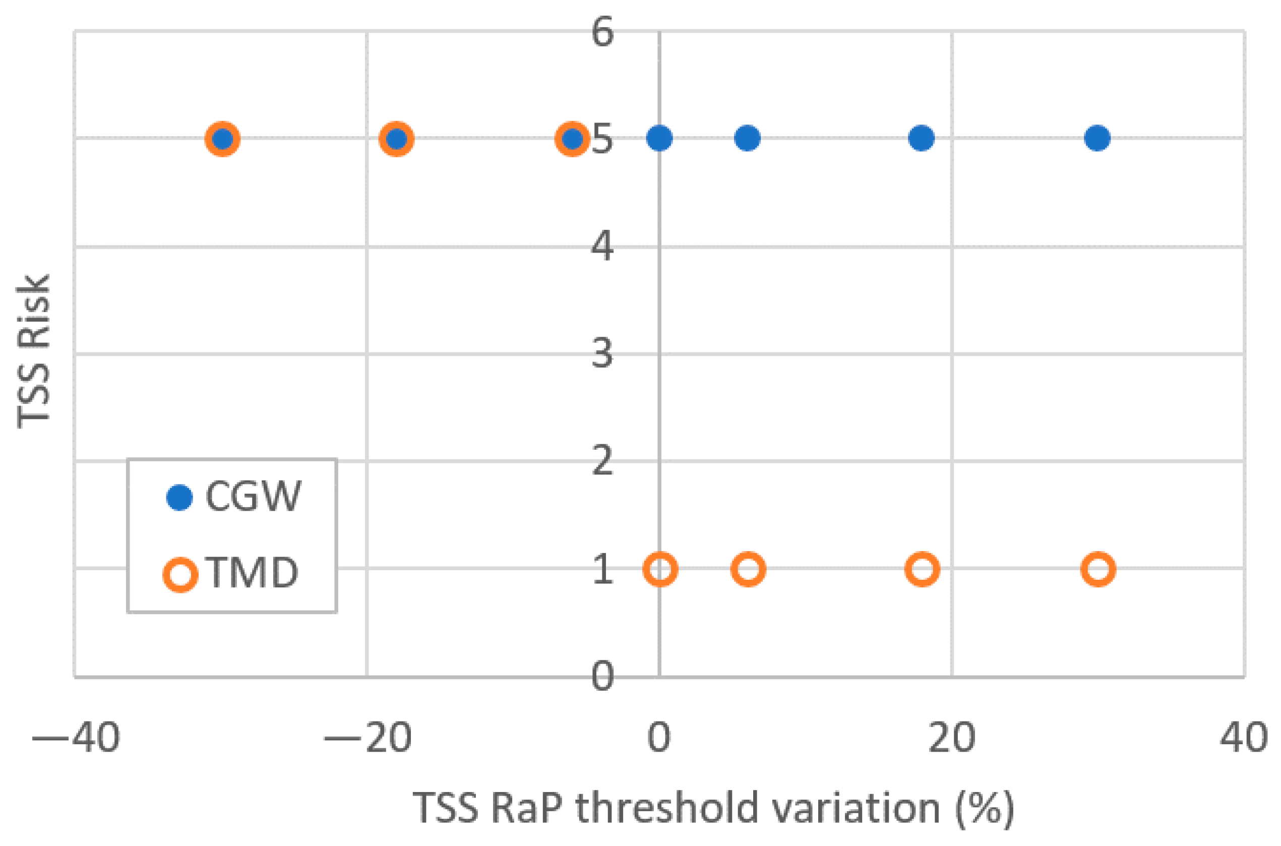
4.6. Sensitivity Analysis, Uncertainty and Future Directions
5. Conclusions
Supplementary Materials
Author Contributions
Funding
Institutional Review Board Statement
Informed Consent Statement
Data Availability Statement
Acknowledgments
Conflicts of Interest
References
- Hrudey, S.E.; Hrudey, E.J.; Pollard, S.J. Risk management for assuring safe drinking water. Environ. Int. 2006, 32, 948–957. [Google Scholar] [CrossRef] [PubMed] [Green Version]
- NHMRC. Australian Drinking Water Guidelines; Commonwealth of Australia; NHMRC: Canberra, Australia, 2011.
- WHO. Guidelines for Drinking Water Quality, 4th ed.; World Health Organisation: Geneva, Switzerland, 2011; Volume 1. [Google Scholar]
- McDonald, R.I.; Weber, K.F.; Padowski, J.; Boucher, T.; Shemie, D. Estimating watershed degradation over the last century and its impact on water-treatment costs for the world’s large cities. Proc. Natl. Acad. Sci. USA 2016, 113, 9117–9122. [Google Scholar] [CrossRef] [Green Version]
- Phiri, B.J.; Pita, A.B.; Hayman, D.T.; Biggs, P.J.; Davis, M.T.; Fayaz, A.; Canning, A.D.; French, N.P.; Death, R.G. Does land use affect pathogen presence in New Zealand drinking water supplies? Water Res. 2020, 185, 116229. [Google Scholar] [CrossRef]
- Zahedi, A.; Monis, P.; Gofton, A.W.; Oskam, C.L.; Ball, A.; Bath, A.; Bartkow, M.; Robertson, I.; Ryan, U. Cryptosporidium species and subtypes in animals inhabiting drinking water catchments in three states across Australia. Water Res. 2018, 134, 327–340. [Google Scholar] [CrossRef] [Green Version]
- Grinham, A.; Gibbes, B.; Gale, D.; Watkinson, A.; Bartkow, M. Extreme rainfall and drinking water quality: A regional perspective. In WIT Transactions on Ecology and the Environment; WIT Press: Chilworth, UK, 2012; Volume 164, pp. 183–194. [Google Scholar]
- LeChevallier, M.W.; Au, K.K. Water Treatment and Pathogen Control: Process Efficiency in Achieving Safe Drinking Water; IWA Publishing: London, UK, 2004. [Google Scholar]
- Collins, K.E.; Doscher, C.; Rennie, H.G.; Ross, J.G. The effectiveness of riparian ‘restoration’ on water quality—A case study of lowland streams in Canterbury, New Zealand. Restor. Ecol. 2013, 21, 40–48. [Google Scholar] [CrossRef]
- Olley, J.; Burton, J.; Hermoso, V.; Smolders, K.; McMahon, J.; Thomson, B.; Watkinson, A. Remnant riparian vegetation, sediment and nutrient loads, and river rehabilitation in subtropical Australia. Hydrol. Process. 2015, 29, 2290–2300. [Google Scholar] [CrossRef]
- Maseyk, F.J.F.; Dominati, E.J.; Mackay, A.D. Change in ecosystem service provision within a lowland dairy landscape under different riparian margin scenarios. Int. J. Biodivers. Sci. Ecosyst. Serv. Manag. 2018, 14, 17–31. [Google Scholar] [CrossRef] [Green Version]
- Billington, K.; Deere, D. On-Site Wastewater Management: Mount Lofty Ranges, South Australia-Reducing water quality risks from septic tanks in a watershed catchment. Water-Aust. Water Wastewater Assoc. 2012, 39, 106. [Google Scholar]
- Kay, D.; Crowther, J.; Kay, C.; McDonald, A.; Ferguson, C.; Stapleton, C.; Wyer, M. Effectiveness of best management practices for attenuating the transport of livestock-derived pathogens within catchments. In Animal Waste, Water Quality and Human Health; Dufour, A., Bartram, J., Bos, R., Gannon, V., Eds.; IWA Publishing: London, UK, 2012; pp. 195–255. [Google Scholar]
- Palmer, M.A.; Menninger, H.L.; Bernhardt, E. River restoration, habitat heterogeneity and biodiversity: A failure of theory or practice? Freshw. Biol. 2010, 55, 205–222. [Google Scholar] [CrossRef]
- Hermoso, V.; Pantus, F.; Olley, J.; Linke, S.; Mugodo, J.; Lea, P. Systematic planning for river rehabilitation: Integrating multiple ecological and economic objectives in complex decisions. Freshw. Biol. 2012, 57, 1–9. [Google Scholar] [CrossRef] [Green Version]
- Tulloch, V.J.; Tulloch, A.I.; Visconti, P.; Halpern, B.S.; Watson, J.E.; Evans, M.C.; Auerbach, N.A.; Barnes, M.; Beger, M.; Chadès, I. Why do we map threats? Linking threat mapping with actions to make better conservation decisions. Front. Ecol. Environ. 2015, 13, 91–99. [Google Scholar] [CrossRef] [Green Version]
- Argent, R.M.; Perraud, J.-M.; Rahman, J.M.; Grayson, R.B.; Podger, G.M. A new approach to water quality modelling and environmental decision support systems. Environ. Model. Softw. 2009, 24, 809–818. [Google Scholar] [CrossRef]
- McIntosh, B.S.; Ascough II, J.C.; Twery, M.; Chew, J.; Elmahdi, A.; Haase, D.; Harou, J.J.; Hepting, D.; Cuddy, S.; Jakeman, A.J. Environmental decision support systems (EDSS) development—Challenges and best practices. Environ. Model. Softw. 2011, 26, 1389–1402. [Google Scholar] [CrossRef]
- Volk, M.; Lautenbach, S.; van Delden, H.; Newham, L.T.; Seppelt, R. How can we make progress with decision support systems in landscape and river basin management? Lessons learned from a comparative analysis of four different decision support systems. Environ. Manag. 2010, 46, 834–849. [Google Scholar] [CrossRef]
- Linke, S.; Kennard, M.J.; Hermoso, V.; Olden, J.D.; Stein, J.; Pusey, B.J. Merging connectivity rules and large-scale condition assessment improves conservation adequacy in river systems. J. Appl. Ecol. 2012, 49, 1036–1045. [Google Scholar] [CrossRef] [Green Version]
- Langhans, S.D.; Hermoso, V.; Linke, S.; Bunn, S.E.; Possingham, H.P. Cost-effective river rehabilitation planning: Optimizing for morphological benefits at large spatial scales. J. Environ. Manag. 2014, 132, 296–303. [Google Scholar] [CrossRef]
- Carr, R.; Podger, G. eWater source—Australia’s next generation IWRM modelling platform. In Proceedings of the 34th Hydrology and Water Resources Symposium, Sydney, Australia, 19–22 November 2012; pp. 742–749. [Google Scholar]
- Fu, B.; Merritt, W.S.; Croke, B.F.W.; Weber, T.R.; Jakeman, A.J. A review of catchment-scale water quality and erosion models and a synthesis of future prospects. Environ. Model. Softw. 2019, 114, 75–97. [Google Scholar] [CrossRef]
- Neitsch, S.L.; Arnold, J.G.; Kiniry, J.R.; Williams, J.R. Soil and Water Assessment Tool Theoretical Documentation Version 2009; Texas Water Resources Institute: College Station, TX, USA, 2011. [Google Scholar]
- Bicknell, B.; Imhoff, J.; Kittle, J., Jr.; Jobes, T.; Donigian, A., Jr.; Johanson, R. Hydrological Simulation Program–FORTRAN (HSPF): User’s Manual for Version 12; US Environmental Protection Agency: Athens, GA, USA, 2001.
- Wilson, E.; Butterfield, D. A semi-distributed Integrated Nitrogen model for multiple source assessment in Catchments (INCA): Part I—Model structure and process equations. Sci. Total Environ. 1998, 210, 547–558. [Google Scholar]
- Dai, C.; Qin, X.S.; Tan, Q.; Guo, H.C. Optimizing best management practices for nutrient pollution control in a lake watershed under uncertainty. Ecol. Indic. 2018, 92, 288–300. [Google Scholar] [CrossRef]
- Herman, M.R.; Nejadhashemi, A.P.; Daneshvar, F.; Ross, D.M.; Woznicki, S.A.; Zhang, Z.; Esfahanian, A.-H. Optimization of conservation practice implementation strategies in the context of stream health. Ecol. Eng. 2015, 84, 1–12. [Google Scholar] [CrossRef]
- Shin, H.; Joo, C.; Koo, J. Optimal rehabilitation model for water pipeline systems with genetic algorithm. Procedia Eng. 2016, 154, 384–390. [Google Scholar] [CrossRef] [Green Version]
- Luna, T.; Ribau, J.; Figueiredo, D.; Alves, R. Improving energy efficiency in water supply systems with pump scheduling optimization. J. Clean. Prod. 2019, 213, 342–356. [Google Scholar] [CrossRef]
- Vasan, A.; Raju, K.S. Comparative analysis of Simulated Annealing, Simulated Quenching and Genetic Algorithms for optimal reservoir operation. Appl. Soft Comput. 2009, 9, 274–281. [Google Scholar] [CrossRef]
- Nicklow, J.; Reed, P.; Savic, D.; Dessalegne, T.; Harrell, L.; Chan-Hilton, A.; Karamouz, M.; Minsker, B.; Ostfeld, A.; Singh, A. State of the art for genetic algorithms and beyond in water resources planning and management. J. Water Resour. Plan. Manag. 2010, 136, 412–432. [Google Scholar] [CrossRef]
- Santé-Riveira, I.; Crecente-Maseda, R.; Miranda-Barrós, D. GIS-based planning support system for rural land-use allocation. Comput. Electron. Agric. 2008, 63, 257–273. [Google Scholar] [CrossRef]
- Aerts, J.C.; Heuvelink, G.B. Using simulated annealing for resource allocation. Int. J. Geogr. Inf. Sci. 2002, 16, 571–587. [Google Scholar] [CrossRef] [Green Version]
- Merritt, W.S.; Fu, B.; Ticehurst, J.L.; El Sawah, S.; Vigiak, O.; Roberts, A.M.; Dyer, F.; Pollino, C.A.; Guillaume, J.H.; Croke, B.F. Realizing modelling outcomes: A synthesis of success factors and their use in a retrospective analysis of 15 Australian water resource projects. Environ. Model. Softw. 2017, 94, 63–72. [Google Scholar] [CrossRef]
- Walling, E.; Vaneeckhaute, C. Developing successful environmental decision support systems: Challenges and best practices. J. Environ. Manag. 2020, 264, 110513. [Google Scholar] [CrossRef] [PubMed]
- Waterhouse, J.; Brodie, J.; Lewis, S.; Mitchell, A. Quantifying the sources of pollutants in the Great Barrier Reef catchments and the relative risk to reef ecosystems. Mar. Pollut. Bull. 2012, 65, 394–406. [Google Scholar] [CrossRef]
- Kroon, F.J.; Kuhnert, P.M.; Henderson, B.L.; Wilkinson, S.N.; Kinsey-Henderson, A.; Abbott, B.; Brodie, J.E.; Turner, R.D. River loads of suspended solids, nitrogen, phosphorus and herbicides delivered to the Great Barrier Reef lagoon. Mar. Pollut. Bull. 2012, 65, 167–181. [Google Scholar] [CrossRef]
- Queensland Government State Office. Queensland Government Population Projections, 2018th ed.; Queensland SA4s. Available online: http://www.qgso.qld.gov.au (accessed on 5 December 2020).
- Thompson, C.; Croke, J.; Fryirs, K.; Grove, J. A channel evolution model for subtropical macrochannel systems. CATENA 2016, 139, 199–213. [Google Scholar] [CrossRef]
- Ferguson, C. Deterministic Model of Microbil Sources, Fate and Transport: A Quantitative Tool for Pathogen Catchment Budgeting. Ph.D. Thesis, The University of New South Wales, New South Wales, Australia, June 2005. [Google Scholar]
- Ferguson, C.; Kay, D. Transport of microbial pollution in catchment systems. In Animal Waste, Water Quality and Human Health; Dufour, A., Bartram, J., Bos, R., Gannon, V., Eds.; IWA Publishing: London, UK, 2012; pp. 157–193. [Google Scholar]
- Baker, D.; Ferguson, C.; Chier, P.; Warnecke, M.; Watkinson, A. Standardised survey method for identifying catchment risks to water quality. J. Water Health 2016, 14, 349–368. [Google Scholar] [CrossRef] [Green Version]
- Gill, M.A. Sedimentation and useful life of reservoirs. J. Hydrol. 1979, 44, 89–95. [Google Scholar] [CrossRef]
- Searcy, K.E.; Packman, A.I.; Atwill, E.R.; Harter, T. Deposition of Cryptosporidium oocysts in streambeds. Appl. Environ. Microbiol. 2006, 72, 1810–1816. [Google Scholar] [CrossRef] [PubMed] [Green Version]
- Olley, J.; Burton, J.; Smolders, K.; Pantus, F.; Pietsch, T. The application of fallout radionuclides to determine the dominant erosion process in water supply catchments of subtropical South-east Queensland, Australia. Hydrol. Process. 2013, 27, 885–895. [Google Scholar] [CrossRef]
- Garzon-Garcia, A.; Olley, J.M.; Bunn, S.E.; Moody, P. Gully erosion reduces carbon and nitrogen storage and mineralization fluxes in a headwater catchment of south-eastern Queensland, Australia. Hydrol. Process. 2014, 28, 4669–4681. [Google Scholar] [CrossRef]
- Hancock, H.; Caitcheon, G. Sediment Sources and Transport to the Logan-Albert Estuary during the January 2008 Flood Event; CSIRO: Clayton, Australia, 2010.
- Khan, S.J.; Deere, D.; Leusch, F.D.L.; Humpage, A.; Jenkins, M.; Cunliffe, D. Extreme weather events: Should drinking water quality management systems adapt to changing risk profiles? Water Res. 2015, 85, 124–136. [Google Scholar] [CrossRef]
- Hrudey, S.E.; Hrudey, E.J. Published Case Studies of Waterborne Disease Outbreaks—Evidence of a Recurrent Threat. Water Environ. Res. 2007, 79, 233–245. [Google Scholar] [CrossRef]


| WTP | Supplies | Sub-Catchment Area (km2) | Number of Planning Units | Planning Unit Area µ(σ)(ha) |
|---|---|---|---|---|
| TMD | Maroon Dam | 106 | 8 | 1323 (662) |
| TRA | Rathdowny | 534 | 26 | 2052 (1849) |
| TKO | Kooralbyn | 1035 | 47 | 2202 (1698) |
| TBE | Beaudesert | 1385 | 61 | 2270 (1663) |
| CGW | Beaudesert, Water grid | 2381 | 130 | 1832 (1446) |
| TCN | Canungra | 92 | 4 | 2298 (1435) |
| Hazardous Process | Hazard | |||
|---|---|---|---|---|
| TSS | Bacteria | Protozoa | Viral | |
| Hillslope erosion | ✓ | - | - | - |
| Landslides | ✓ | - | - | - |
| Gully erosion | ✓ | - | - | - |
| Channel (bank) erosion | ✓ | - | - | - |
| Unsealed roads | ✓ | - | - | - |
| Point source (instream sand and gravel extraction) | ✓ | - | - | - |
| Livestock grazing | - | ✓ | ✓ | - |
| Intensive livestock industries | - | ✓ | ✓ | - |
| Sewerage Treatment Plants | - | ✓ | ✓ | ✓ |
| On-site Sewerage Facilities | - | ✓ | ✓ | ✓ |
| Stormwater | - | ✓ | ✓ | ✓ |
| Aquatic recreation | - | ✓ | ✓ | ✓ |
| Program | Intervention | Efficacy |
|---|---|---|
| Channel erosion | Earthworks/rockwork/fencing—basic and complex | 90% |
| Revegetation and fencing | 90% & 1 LRV | |
| Revegetation | 60% | |
| Livestock exclusion fencing | 75% & 1 LRV | |
| Broadscale Livestock & Riparian Manag. | Earthworks basic | 90% |
| Revegetation | 60% | |
| Livestock exclusion fencing | 75% & 1 LRV | |
| Revegetation and fencing | 90% & 3 LRV | |
| Fencing and off-stream watering | 75% & 3 LRV | |
| Revegetation, fencing and off-stream watering | 90% & 3 LRV | |
| Gully erosion | Earthworks/rockwork/fencing—basic and complex | 90% |
| Revegetation with grasses | 60% | |
| Livestock exclusion fencing | 75% | |
| Revegetation and fencing | 90% | |
| Landslides | Earthworks complex | 90% |
| Earthworks simple swales or contours | 90% | |
| Earthworks and fencing | 90% | |
| Revegetation with woody species | 75% | |
| Revegetation and fencing | 90% | |
| Livestock exclusion fencing | 10% | |
| Point sources | Revegetation with grass filter strips | 80% |
| Revegetation and fencing | 90% | |
| Sediment detention dam (small, large, complex) | 50, 60 & 75% | |
| Intensive livestock effluent manag. | Fencing to exclude calves from water course | 60% & 1 LRV |
| Laneways | 60% & 1 LRV | |
| Stream crossings | 60% | |
| Feedpad—hardening with basic or advanced drainage | 10, 20% & 1,2 LRV | |
| Effluent pump upgrade and primary treatment (solids trap) | 50% & 1 †,2 ‡ LRV | |
| Secondary treatment | 60% & 1 †,2 ‡ LRV | |
| Effluent pump upgrade, primary treatment (solids trap) + irrigation | 60% & 2 †,3 ‡ LRV | |
| Effluent pump upgrade, primary treatment (solids trap) + Secondary + irrigation | 60% & 3 †,4 ‡ LRV |
| Risk | Descriptor | TSS (t/Year) | Viral (log10 Particles/Day) | Bacteria (log10 Organisms/Day) | Protozoa (log10 Oocysts/Day) |
|---|---|---|---|---|---|
| 1 | Insignificant | <343 | <4 | <4 | <3.5 |
| 2 | Minor | 343 < 521 | 4 < 5 | 4 < 5 | 3.5 < 4.5 |
| 3 | Moderate | 521 < 906 | 5 < 6 | 5 < 6 | 4.5 < 5.5 |
| 4 | Major | 906 < 2070 | 6 < 8 | 6 < 8 | 5.5 < 7.5 |
| 5 | Catastrophic | >2070 | >8 | >8 | >7.5 |
| WTP | Source Catchment | Excluding Nested WTP |
|---|---|---|
| TCN | 1% | 1% |
| TMD | <1% | <1% |
| TRA | 8% | 7% |
| TKO | 22% | 14% |
| TBE | 41% | 19% |
| CGW | 99% | 58% |
| Program | Percent of Budget Cost |
|---|---|
| Channel erosion and riparian management interventions | 44% |
| Gully interventions | 9% |
| Landslide interventions | 1% |
| Intensive livestock interventions | 46% |
Publisher’s Note: MDPI stays neutral with regard to jurisdictional claims in published maps and institutional affiliations. |
© 2021 by the authors. Licensee MDPI, Basel, Switzerland. This article is an open access article distributed under the terms and conditions of the Creative Commons Attribution (CC BY) license (http://creativecommons.org/licenses/by/4.0/).
Share and Cite
Thompson, C.; Stewart, M.; Marsh, N.; Phung, V.; Lynn, T. A Planning Tool for Optimizing Investment to Reduce Drinking Water Risk to Multiple Water Treatment Plants in Open Catchments. Water 2021, 13, 531. https://doi.org/10.3390/w13040531
Thompson C, Stewart M, Marsh N, Phung V, Lynn T. A Planning Tool for Optimizing Investment to Reduce Drinking Water Risk to Multiple Water Treatment Plants in Open Catchments. Water. 2021; 13(4):531. https://doi.org/10.3390/w13040531
Chicago/Turabian StyleThompson, Chris, Morag Stewart, Nick Marsh, Viet Phung, and Thomas Lynn. 2021. "A Planning Tool for Optimizing Investment to Reduce Drinking Water Risk to Multiple Water Treatment Plants in Open Catchments" Water 13, no. 4: 531. https://doi.org/10.3390/w13040531
APA StyleThompson, C., Stewart, M., Marsh, N., Phung, V., & Lynn, T. (2021). A Planning Tool for Optimizing Investment to Reduce Drinking Water Risk to Multiple Water Treatment Plants in Open Catchments. Water, 13(4), 531. https://doi.org/10.3390/w13040531