Deep Learning with Long Short Term Memory Based Sequence-to-Sequence Model for Rainfall-Runoff Simulation

Abstract

Accurate runoff prediction is one of the important tasks in various fields such as agriculture, hydrology, and environmental studies. Recently, with massive improvements of computational system and hardware, the deep learning-based approach has recently been applied for more accurate runoff prediction. In this study, the long short-term memory model with sequence-to-sequence structure was applied for hourly runoff predictions from 2015 to 2019 in the Russian River basin, California, USA. The proposed model was used to predict hourly runoff with lead time of 1–6 h using runoff data observed at upstream stations. The model was evaluated in terms of event-based performance using the statistical metrics including root mean square error, Nash-Sutcliffe Efficiency, peak runoff error, and peak time error. The results show that proposed model outperforms support vector machine and conventional long short-term memory models. In addition, the model has the best predictive ability for runoff events, which means that it can be effective for developing short-term flood forecasting and warning systems. The results of this study demonstrate that the deep learning-based approach for hourly runoff forecasting has high predictive power and sequence-to-sequence structure is effective method to improve the prediction results.

1. Introduction

Accurate rainfall-runoff simulation is an essential task for proper strategies for floods, droughts and water resources management [1,2,3,4]. Various approaches, including conceptual model, physics-based model, and data-driven method, have been applied to simulate the nonlinear rainfall-runoff relationship. These methods can be used in multiple time-steps from short-term simulations to long-term simulations for various challenges such as developing flood forecasting and warning system, drought analysis, and water resources management [5,6,7,8].

The physics-based model contains a lot of parameters and requires a model calibration process to minimize uncertainty and to obtain high accuracy of outputs. However, different results can be obtained from physics-based models due to uncertainty in model structure and parameter calculation [3,9,10]. In addition, some physically based models have a limitation in that it is difficult to consider all of meteorological, topographic, and geological effects in the process of simplifying a complex hydrologic system, and accumulation of errors during the calculation process due to the internal uncertainty involved [11,12,13,14,15]. Data-driven models are known as an effective alternative to overcome these limitations of physics-based models. In addition, since accurate simulation for a hydrological cycle requires a highly intensive computation process, simple and practical methods for hydrological analysis with minimum requirement are needed [3].

Recently, data-driven models, which are based on functional relationships between independent and dependent variables, have significantly contributed to analyze hydrological cycles [16]. Typical types of machine learning-based data-driven models for hydrological analysis include artificial neural networks (ANN) [17], support vector machine (SVM) [18], and random forest models (RF) [19]. Most recently, deep learning-based data-driven models, such as convolutional neural networks (CNN) [20], recurrent neural network (RNN) [21], and long short-term memory (LSTM) [22,23], have been used in hydrological studies. These models have demonstrated high predictive performance with fewer parameters than physically based models [16,24]. Moreover, these models can be directly trained based on patterns from a huge number of datasets without using physical theories or making strong structural assumptions [23].

In the field of hydrology, many studies have used various types of data-driven models for hydrological prediction, such as runoff, precipitation, soil property, and river stages [25,26,27,28,29,30,31]. In addition, various models based on machine learning, including ANN, SVM, and RF have been applied for rainfall-runoff simulation, and it was found that these models can be effective alternatives to physical based models [32,33,34,35,36,37]. For example, Tayfur and Singh [32] tested data-driven models‘ performance for simulating event-based rainfall-runoff relationship. They used an ANN model with fuzzy logic for runoff simulation and concluded that these models can satisfactorily predict event-based runoff hydrographs. Muñoz et al. [35] used RF model for flash-flood forecasting in the mountain catchment. They showed improved prediction results with optimal input selection process.

Moreover, many previous studies have used deep learning-based data-driven models, which have been developed recently, for hydrological prediction and simulations [38,39,40,41,42]. Assem et al. [38] applied deep convolutional neural networks for long-term prediction for water flow and water level and showed how the proposed model can be used for water authorities for various fields. Kratzert et al. [40] used an LSTM network model for rainfall-runoff modelling and showed the potential of the LSTM model as a regional hydrological model for a variety of regions. They showed the better performance of LSTM model than physics-based hydrological model for prediction of discharge. In addition, Mok et al. [41] showed the potential of LSTM model for predicting the hourly inflow of the multipurpose dam. They found that the LSTM model can provide high accuracy of inflow predictions with historic datasets of precipitation and inflows. With the improvement of computational system and resources, the deep learning-based models have been emerged to simulate rainfall-runoff process using various datasets such as ground-based observations, remote sensing-based data. In addition, the deep learning-based model has improved prediction accuracy compared to the other approaches, but has a limitation in not considering the temporal dependence that can reflect the variability relationship of time-series data at different time frequencies.

Cho et al. [43] and Sutskever et al. [44] presented improved language translation results through learning of the model using a sequence-to-sequence structure that can consider temporal dependence on LSTM (LSTM-s2s). In the hydrological study, there have been insufficient studies that used LSTM-s2s model for hydrological predictions. Thus, this study developed a hourly runoff prediction approach using LSTM-s2s model for runoff prediction which is significant for proper flood forecasting in the Russian River basin, California. In addition, predicted results of LSTM-s2s model were compared with other models such as SVM and traditional LSTM models to demonstrate the predictive power of the LSTM-s2s model for runoff prediction. The objectives of this study are to: (1) develop hourly runoff prediction approach using LSTM-s2s model; (2) compare the predictive performance of LSTM-s2s with other data-driven models (e.g., traditional SVM and LSTM models); and (3) evaluate event-based predictive performance of proposed model. The results of this study are expected to present information of LSTM-s2s model, which is rarely applied to the hydrology study. In addition, better understandings of potential LSTM-s2s model will be provided in this study.

2. Materials and Methods

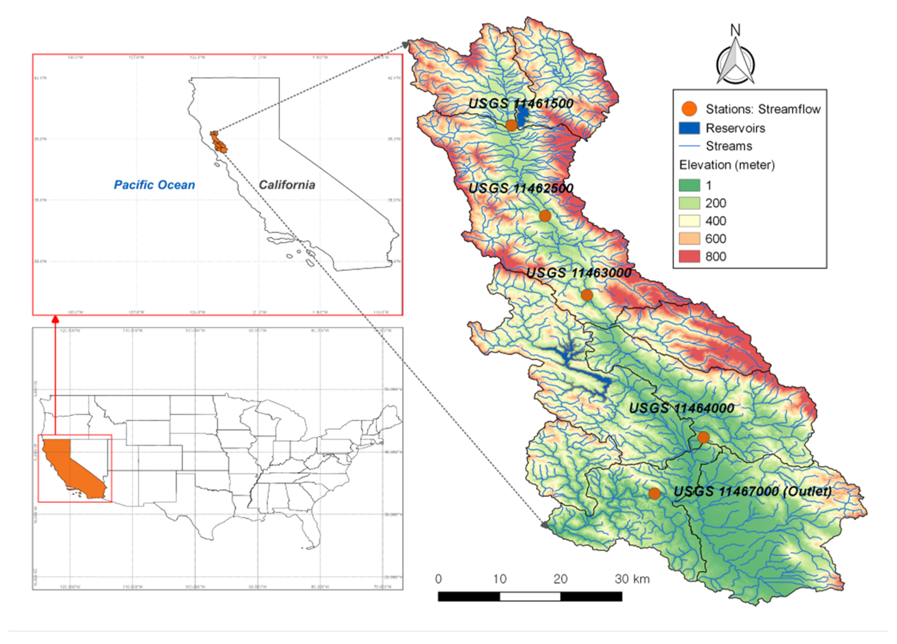
2.1. Study Area and Data

The Russian River basin (latitude 39.38° N, longitude −123.23° W) is located in northern California. The drainage area of Russian River basin is 3846 km² (Figure 1), covering northern Sonoma County and southern Mendocino County. Due to the unique geography and proximity to the coast, the Russian River basin has challenges related to flood mitigation, water resource management, water quality, and soil erosions [45]. In addition, this area has a complex terrain with the land cover/use dominated by evergreen forest, deciduous forest, shrub/scrub, and grassland [45]. In this area are located two reservoirs, Mendocino and Sonoma, which are regulated by the Coyote Valley and Warm Springs dams. The Russian River basin is located on the west coast of the United States with an average annual precipitation of 1180 mm and more than 80% of its annual precipitation was observed during wet season (from November to March). The Russian River basin is affected by various meteorological factors such as extratropical cyclones, jet streams, and atmospheric rivers from the Pacific oceans [46]. For runoff forecasting at outlet point, hourly runoff data were obtained from five United States Geological Survey (USGS) stations (Station ID: 11461500; 11462500; 11463000; 11464000; and 11467000) for the period from 2015 to 2019. Generally, 70–80% of the available datasets are allocated for training and the remaining 20–30% of data are partitioned for testing [47]. In this study, the training period is from January 2015 to December 2018 (80%) and the test period is from January 2019 to December 2019 (20%).

2.2. Data-Driven Models

2.2.1. Support Vector Machine

The Support Vector Machine (SVM) model, presented by Vapnik [18], is one of the data-driven models which are widely used for classification and regression analysis. The SVM model classifies different classes of datasets using maximum margin for the distance between data points and optimal classification is determined by optimal hyperplane composed of support vectors.

Support vector machines can apply kernel functions to map original data into a higher dimension and to the input for minimizing the ε-insensitive loos function [48]. The typical kernel functions include Polynomial, Sigmoid, and Radial Basis Function (RBF). This study used the RBF to SVM model since it is a very popular kernel function used in SVM model and shows high reliability [48]. The SVM model is applicable not only to classification but also to regression for prediction by applying an ε-insensitive loss function to the SVM. This type of model is called Support Vector Regression (SVR) [49], and it was used for runoff prediction in this study.

The basic theory of SVR is to find the flattest regression function, f(x), so that the target variable of the given dataset is within the deviation ε. The optimal regression function, f(x), is used to minimize error using the optimization equation and constraints that find the flattest function indicated in Equations (1)–(3) [49].

$$\mathrm{f}\left(\mathrm{x}\right)= \langle \mathrm{w}, \mathrm{x}\rangle +\mathrm{b}$$

(1)

$$\mathrm{minimum} \frac{1}{2}\left|\right|{\mathrm{w}}^2\left|\right|+\mathrm{C}\sum \left({\mathsf{\xi }}_{\mathrm{i}}+{\mathsf{\xi }}_{\mathrm{i}}^{*}\right)$$

(2)

$$\mathrm{subject} \mathrm{to} \{\begin{array}{c}{\mathrm{y}}_{\mathrm{i}}-\langle \mathrm{w},{\mathrm{x}}_{\mathrm{i}}\rangle -\mathrm{b}\le \mathsf{\epsilon }+{\mathsf{\xi }}_{\mathrm{i}}\\ \langle \mathrm{w},{\mathrm{x}}_{\mathrm{i}}\rangle +\mathrm{b}-{\mathrm{y}}_{\mathrm{i}}\le \mathsf{\epsilon }+{\mathsf{\xi }}_{\mathrm{i}}^{*}\end{array} ,{ \mathsf{\xi }}_{\mathrm{i}},{ \mathsf{\xi }}_{\mathrm{i}}^{*} \ge 0$$

(3)

where C represents a penalty value which can determine how many data points are greater than the deviation (e.g., ε). A high value of C is able to reduce the data that deviates from the deviation, while a high value of C causes the overfitting problem. Therefore, finding the optimal C value is needed for developing a good performance SVR model. The optimization problem to find the optimal function can be solved through the Lagrange function from Equations (2) and (3).

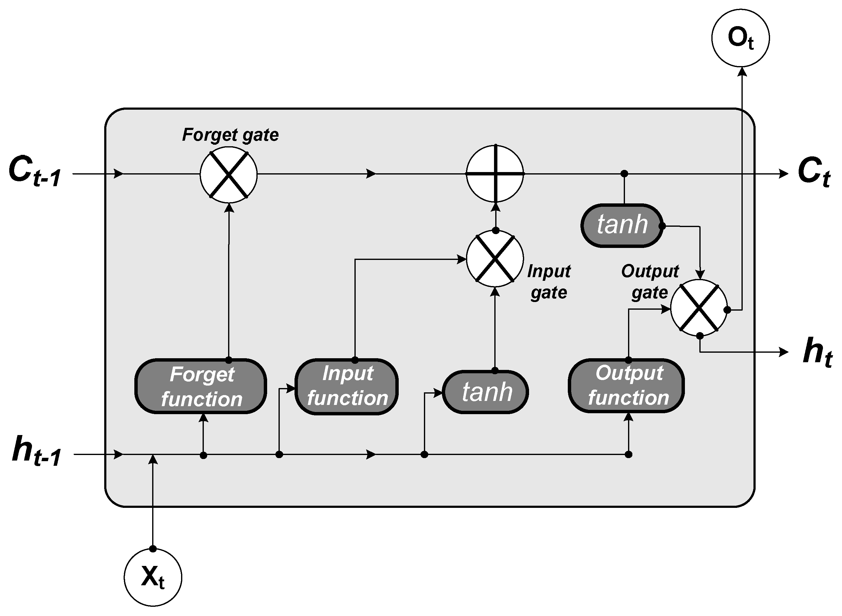
2.2.2. Long Short-Term Memory

The long-short term memory (LSTM) model, introduced by Hochreiter and Schmidhuber [22], is one of the deep learning-based data-driven models widely used for analysis of sequences of datasets. LSTM was developed to solve the problem of gradient vanishing or gradient exploding of the error slope in the recurrent neural network when analyzing long-term datasets. Figure 2 shows the structure and conceptual diagram of LSTM.

The LSTM model consists of a number of blocks. Each block includes cells representing the state over time, and three non-linear gates that regulate the flow of data: the forget gate (f_t), input gate (i_t), and output gate (O_t). The LSTM computes the algorithms from an input sequence x_t to output O_t by looping through Equations (4)–(9) with initial values of C₀ = 0 and h₀ = 0 [49].

$${\mathrm{f}}_{\mathrm{t}}= \mathsf{\sigma }\left({\mathrm{W}}_{\mathrm{f}}·\left[{\mathrm{h}}_{\mathrm{t}-1},{\mathrm{x}}_{\mathrm{t}}\right]+{\mathrm{b}}_{\mathrm{f}}\right)$$

(4)

$${\mathrm{i}}_{\mathrm{t}}= \mathsf{\sigma }\left({\mathrm{W}}_{\mathrm{i}}·\left[{\mathrm{h}}_{\mathrm{t}-1},{\mathrm{x}}_{\mathrm{t}}\right]+{\mathrm{b}}_{\mathrm{i}}\right)$$

(5)

$${\mathrm{O}}_{\mathrm{t}}= \mathsf{\sigma }\left({\mathrm{W}}_{\mathrm{o}}·\left[{\mathrm{h}}_{\mathrm{t}-1},{\mathrm{x}}_{\mathrm{t}}\right]+{\mathrm{b}}_{\mathrm{o}}\right)$$

(6)

$${\tilde{\mathrm{C}}}_{\mathrm{t}}= \tan \mathrm{h}\left({\mathrm{W}}_{\mathrm{C}}·\left[{\mathrm{h}}_{\mathrm{t}-1},{\mathrm{x}}_{\mathrm{t}}\right]+{\mathrm{b}}_{\mathrm{C}}\right)$$

(7)

$${\mathrm{C}}_{\mathrm{t}}={ \mathrm{f}}_{\mathrm{t}}\times {\mathrm{C}}_{\mathrm{t}-1}+{\mathrm{i}}_{\mathrm{t}}\times {\tilde{\mathrm{C}}}_{\mathrm{t}}$$

(8)

$${\mathrm{h}}_{\mathrm{t}}={ \mathrm{O}}_{\mathrm{t}}\times \tan \mathrm{h}({\mathrm{C}}_{\mathrm{t}})$$

(9)

where σ is the non-linear sigmoid activation function, W_f, W_i, W_o, and W_c represent weight values of forget gate, input gate, output gate, and cells, h_t−1 denotes output data from a previous cell, x_t is current input data and b_f, b_i, and b_o are bias vectors of each gate, respectively. ${\tilde{\mathrm{C}}}_{\mathrm{t}}$ is the state of any cell generated from the activation function. The forget gate aims to determine how much information from the previous block is maintained, the input gate is able to determine which of the new information to store in a cell, and the output gate is used to determine the final output value from the information stored in the cell.

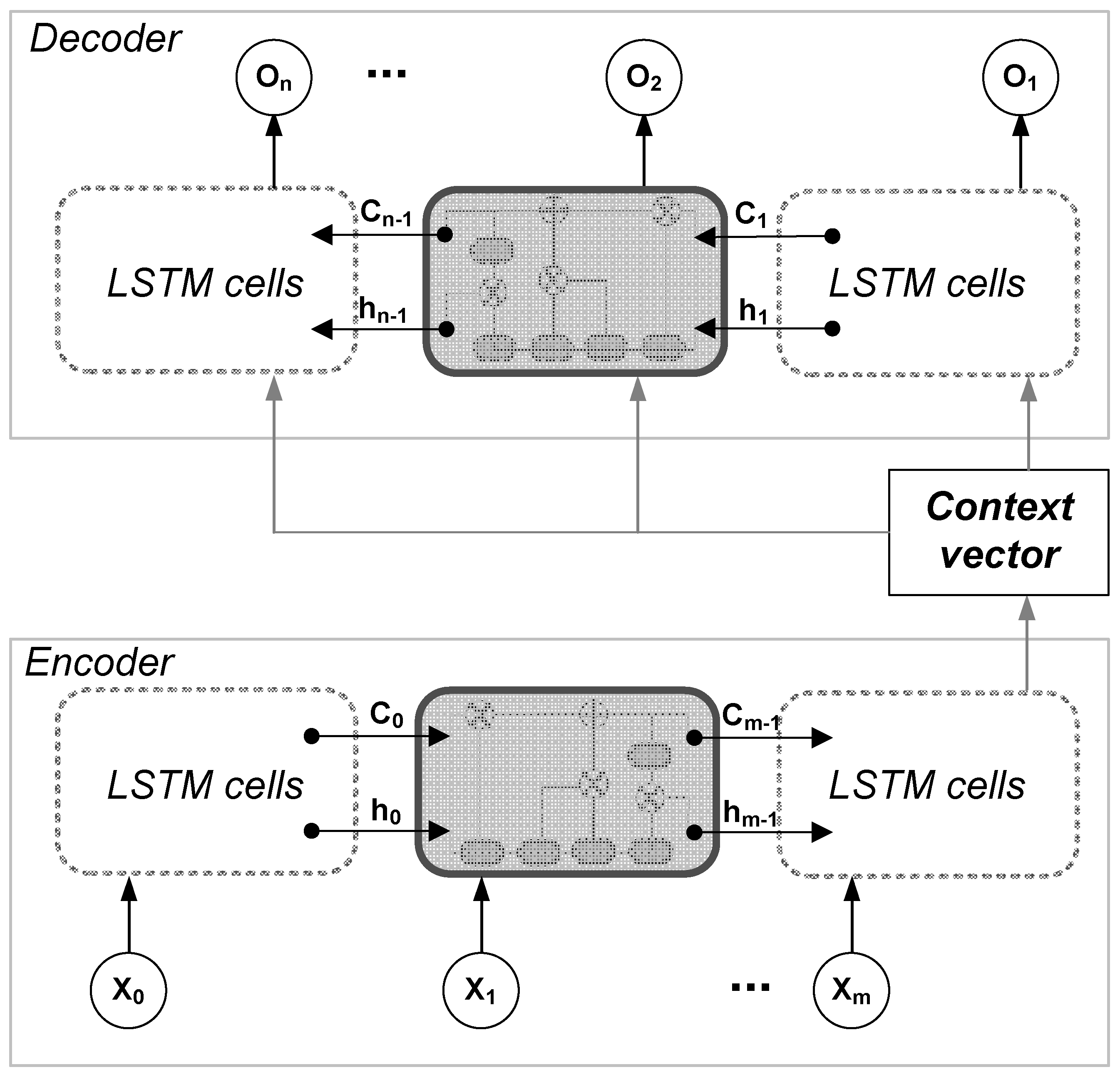
2.2.3. LSTM with Seq2Seq Model

The LSTM model, described in Section 2.2.2, has a limitation that it requires the same time steps for the input and output variables as shown in Figure 2. The LSTM with Seq2Seq (LSMT-s2s) or Encoder-Decoder model, introduced by Cho et al. [43], can overcome this limitation and use different input and output time steps. In the field of hydrology, the LSTM-s2s model can be an effective approach for runoff simulation using rainfall-runoff relationships. According to the Xiang et al. [4], it is essential to consider the precipitation at previous time steps other than the precipitation at the time need to be predicted. Figure 3 shows the conceptual diagram of the LSTM-s2s model.

The LSTM-s2s model is based on a similar process of the traditional LSTM model, but it consists of two structures, encoder and decoder. An encoder LSTM uses the information as input and output from the encoder LSTM with m time steps which can be stored in a one cell named “context vector” and then used as input for the decoder LSTM with n time steps. One of the features of LSTM-s2s models is that the time steps of encoder and decoder LSTM can be different. In this study, X_t represents the observed precipitation and runoff at upstream stations and O_t denotes the predicted runoff.

2.3. Model Development

2.3.1. SVM Model Setup

We applied the SVM model to predict the runoff. The most common kernel functions include linear, polynomial, and radial basis functions. This study used radial basis function as kernel function. One of the most important parameters of the SVM is C value which determines how much data greater than the deviation will be included. In this study, in order to find an optimal value of C, a number of values ranged from 10 to 300 were applied and parameter value indicating best predictive performance was determined. The SVM algorithm with C value of 200 was set.

2.3.2. LSTM-s2s Model Setup

This study used the deep learning-based data-driven models using LSTM and LSTM-s2s models. The LSTM-based models contain three layers with 128 LSTM neurons. A fully connected layer was set up which provides 6 distinct runoff time series. The most common activation functions include tanh, sigmoid, and ReLU functions. In this study, all layers used the ReLU activation function which was found to run faster and obtain better results [4]. For both SVM- and LSTM-based models, the training period is from January 2015 to December 2018 and the test period is from January 2019 to December 2019.

2.3.3. Model Design

This study developed three data-driven models for the hourly runoff prediction of the next 1–6 h. Time series input data include the antecedent runoff with 1–12 h at upstream stations and the outlet station. The collected datasets require pre-processing to supplement the missing values of the data generated during the observation and to enhance data continuity. This supplement process is essential for the LSTM model, as the temporal continuity of the data is important. A missing value was substituted with the average value of the runoff data before and after hours. In this study, data from historic runoff observed at outlet point and coming from four upstream stations were used as input data of data-driven models for runoff prediction at outlet point. The simulation function of runoff is as follows:

$${\mathrm{Runoff}}_{\mathrm{t}+1, \mathrm{t}+2, \dots , \mathrm{t}+6}=\mathrm{f}\left({\mathrm{Runoff}}_{\mathrm{t}-1, \mathrm{t}-2, \dots , \mathrm{t}-12}\&{\mathrm{Upstream}}_{\mathrm{t}-1, \mathrm{t}-2, \dots , \mathrm{t}-12}\right)$$

(10)

2.4. Evaluation Criteria

In this study, four statistics for evaluating the performance of data-driven models are the root mean square error (RMSE), Nash–Sutcliffe Efficiency (NSE), peak runoff error (PRE), and peak time error (PTE).

$$\mathrm{RMSE}= \sqrt{\frac{\sum {\left({\mathrm{y}}_{\mathrm{e}}-{\mathrm{y}}_{\mathrm{o}}\right)}^2}{\mathrm{m}}}$$

(11)

The RMSE ranges from 0 to +∞ and describes how well the simulated value matches to the observed value. The zero value of RMSE means the modelled value is perfect.

$$\mathrm{NSE}= 1 - \frac{\sum {\left({\mathrm{y}}_{\mathrm{e}}-{\mathrm{y}}_{\mathrm{o}}\right)}^2}{\sum {\left({\mathrm{y}}_{\mathrm{o}}-\overline{{\mathrm{y}}_{\mathrm{o}}}\right)}^2}$$

(12)

The NSE represents the predictive power of the model. The NSE ranges from −∞ to 1 and the closer value of 1 means perfect performance of the model and value of less than zero means that the average observed value is better than modelled value.

$$\mathrm{PRE}= \frac{{\mathrm{y}}_{\mathrm{e}, \mathrm{peak}}-{\mathrm{y}}_{\mathrm{o}, \mathrm{peak}}}{{\mathrm{y}}_{\mathrm{o}, \mathrm{peak}}}\times 100 (\%)$$

(13)

where y_e,peak, y_o,peak are the peak values of simulated and observed runoff event. The PRE shows the accuracy of predicted peak value of runoff event from the model.

$$\mathrm{PTE}= \left|{\mathrm{T}}_{\mathrm{e}, \mathrm{peak}}-{\mathrm{T}}_{\mathrm{o}, \mathrm{peak}}\right|$$

(14)

where T_e,peak and T_o,peak denote the time to peak of simulated and observed runoff. The PTE measures the differences between time to peak of simulated and observed runoff.

3. Results and Discussions

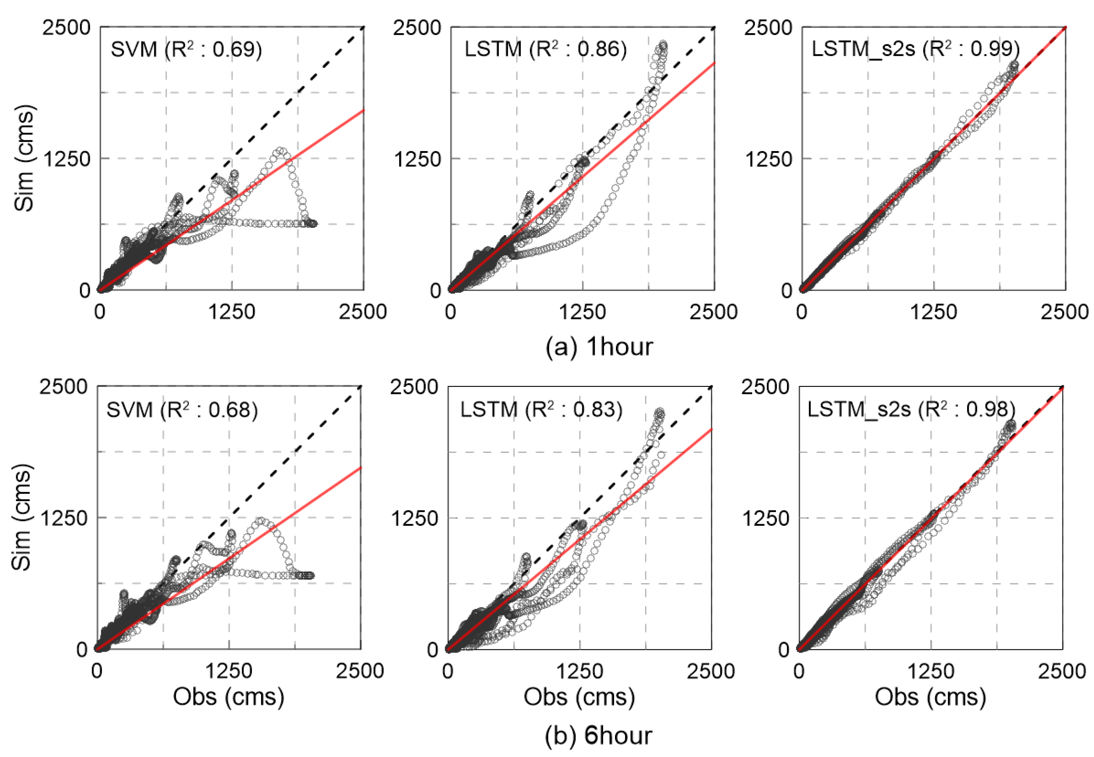
3.1. Overall Performances of Data-Driven Models

In this study, runoff with lead time of 6 h was predicted by three data-driven models of SVM, LSTM, and LSTM-s2s. Even though the rainfall-runoff process is difficult for predicting, these models have shown good performance. Figure 4 shows time-series of the observed and simulated runoff, errors in simulated results with lead time of 1 h. As shown in Figure 4, all three models can simulate the trend of runoff well for the entire test period. The LSTM-s2s model showed more stable and better performance than both of LSTM and SVM models for runoff forecasting. In addition, it was found that the LSTM-s2s model is able to capture the peak of runoff well, while both of LSTM and SVM models have relatively low performances for the period from January 2019–March 2019. In the case of the SVM model, the error in peak of runoff was up to 550 cms, which was 3–4 times that of the other two models. It was also found that the mean values of the error are 8.3% for SVM, 15.7% for LSTM, and 3.7% for LSTM-s2s. The max/min values of the error are 77.9%/−122.4% for SVM, 84.8%/−40.5% for LSTM, and 43.2%/−16.5% for LSTM-s2s. The SVM and LSTM models showed high variability in errors, whereas the LSTM-s2s model provided low variability in errors. Moreover, the LSTM-s2s model has the best predictive ability for hourly runoff forecasting for not only the low-flow period (e.g., April to December) but also the high-flow period (e.g., January to March).

Figure 5 shows the scatter plots of observed and simulated runoff values with lead time of 1 and 6 h. As shown in Figure 5, the R² values of the SVM, LSTM, and LSTM-s2s models are 0.69, 0.86, and 0.99 for lead time of 1 h. There were not significant differences in R² values between lead times of 1 h and 6 h, and the R² values of 6 h are relatively lower than the results of 1 h. Among the three models, the LSTM-s2s model has the highest values of R² indicating that this model can simulate the relationship between simulated and observed runoff. For the runoff below 1250 cms, they are almost near the fit line, which means that these models can provide good performance for prediction of runoff below 1250 cms, while there is uncertainty in runoff prediction above 1250 cms for both SVM and LSTM models, as described in Figure 4.

To compare the performance of three data-driven models for runoff forecasting, this study used two metrics, RMSE and NSE. Figure 6 shows RMSE and NSE resulting from SVM, LSTM, and LSTM-s2s models. As shown in Figure 6a, the RMSE values of both LSTM and LSTM-s2s increase with increasing forecast lead time. The SVM has not significant variations in RMSE value with lead time. Results showed that the LSTM-s2s has the lowest RMSE values for 1–6 h which are about 15–30% of the value of the SVM. In the case of the NSE (Figure 6b), the LSTM-s2s has largest values of the NSE which range from 0.97 to 0.99 for 1–6 h, while the SVM has lowest values below 0.8. Even though all results from these models clearly showed stable and good performance, the LSTM-s2s has the best performance for runoff forecasting for lead time of 1–6 h.

From the results in Figure 4, Figure 5 and Figure 6, it was found that the LSTM-s2s model is a more effective prediction model than other two models. In addition, the LSTM-s2s model can provide predicted hourly runoff regardless of the dry and wet seasons in the Russian River basin.

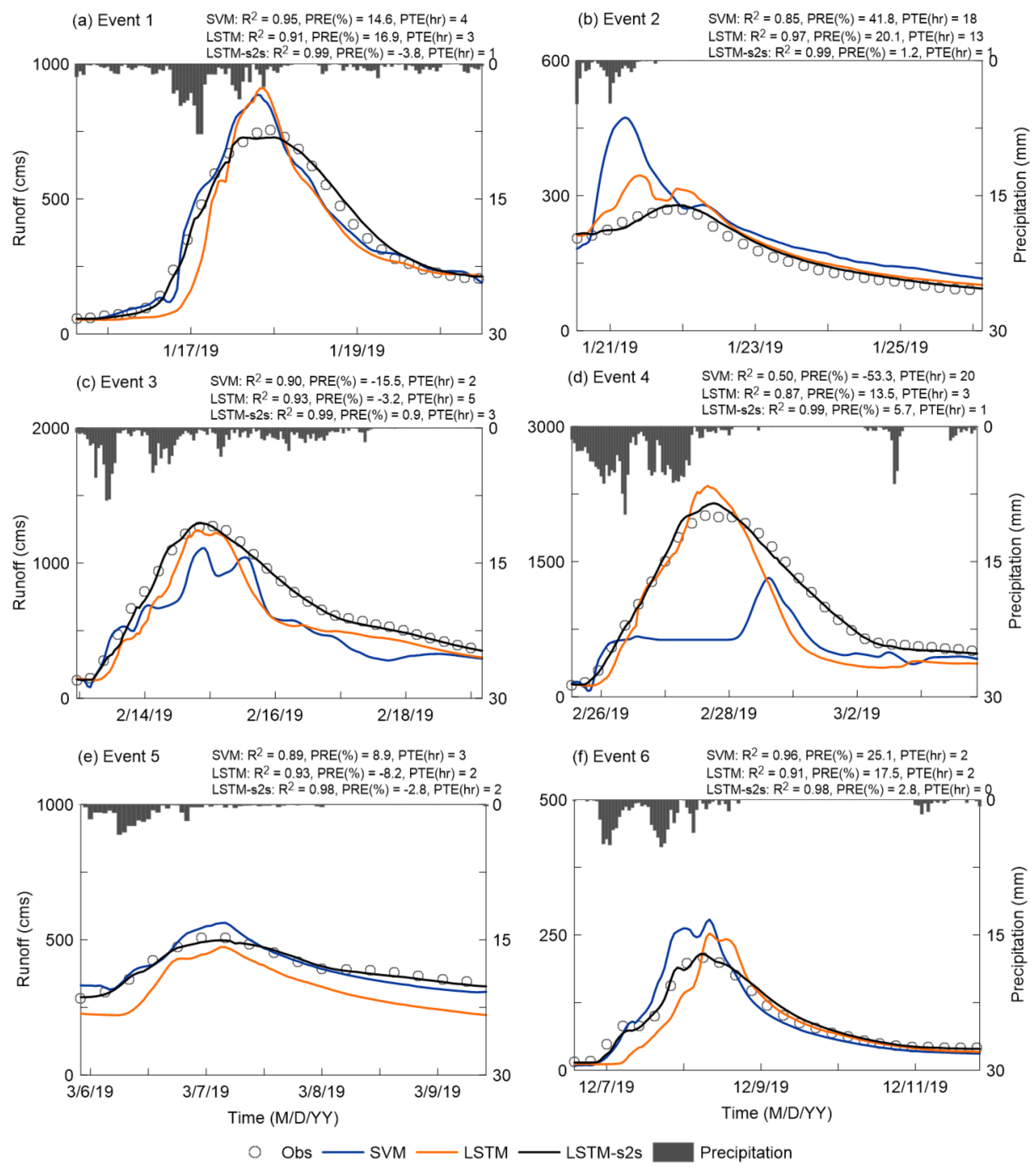
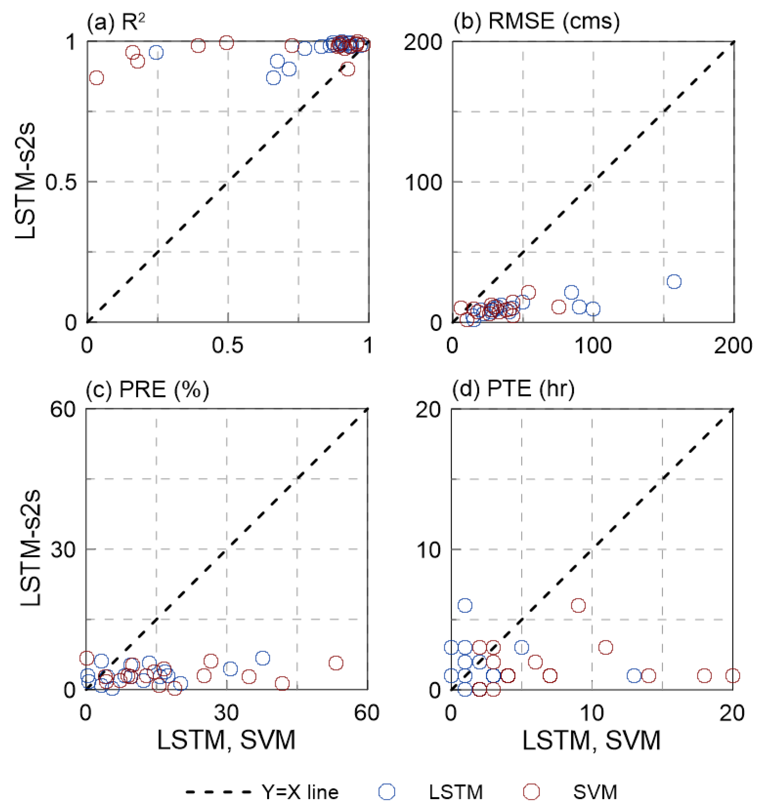
3.2. Event Based Evaluation

In hydrology, the hourly runoff can be used in various fields, including developing flood warning systems and water resources management. Especially, accurate hourly based runoff forecasting is necessary for flood analysis. Besides, accurate prediction of runoff events can be used for mitigating flood damage. For this, this study conducted event-based evaluation of the performance of three data-driven models. There are 17 runoff events simulated from the data-driven models at test stage and Figure 7 shows the observed and predicted 6 hydrographs from the SVM, LSTM, and LSTM-s2s models. To indicate the performance for predicting a runoff event graphically, 6 hydrographs which have the larger peak values and volumes were selected. The peak runoff values of these hydrographs ranged from 250 cms to 2500 cms and peak runoff of event 3, 4 were above 1000 cms.

Among the three models, the SVM model has poor ability for predicting runoff event compared with LSTM-based models. In addition, the LSTM model has relatively poor performance than result from the LSTM-s2s model. In the runoff event 1, 2, and 6, the simulated peak runoff from SVM and LSTM was higher than observations. For event 3, 5, and 6, all models show moderate ability for runoff simulation, while the SVM model shows relatively lower performance for events 2, 4. This study used three metrics, R², PRE, and PTE, to evaluate the event-based simulation performance of the models. The R² values ranged from 0.5–0.95 for SVM, from 0.87–0.97 for LSTM, and from 0.98–0.99 for the LSTM-s2s model. There was significant difference in PRE values between the three models. While the PRE value ranged from −53.3%–41.8% for SVM model, the PRE values of LSTM-based models were under 20%. Moreover, the PTE values indicating an error in peak time ranged from 2–20 h for SVM, from 2–13 h for LSTM, and from 0–3 h for the LSTM-s2s model.

Table 1. Mean values of evaluation metrics for simulated hydrograph events.

Models	Evaluation Metrics
	R2	RMSE (cms)	PRE (Absolute PRE) (%)	PTE (hr)
SVM	0.72	79.5	−7.9 (17.4)	7.0
LSTM	0.82	65.5	−0.4 (11.7)	2.7
LSTM-s2s	0.97	13.4	1.4 (3.1)	1.5

indicates the mean value of evaluation metrics for 17 simulated hydrograph events from the models. As indicated in the table, the LSTM-s2s model has best predictive ability with all evaluation metrics compared to both of SVM and LSTM models. Especially, the LSTM-s2s model has a much lower RMSE value with 13.4 cms than the values of other models which are 79.5 and 65.5 cms. Besides, the LSTM-s2s model shows high performance for simulating peak runoff and time with errors in 3.1% and 1.5 h. Compared with the SVM, LSTM, and LSTM-s2s models, it was found that the LSTM-s2s can be more efficient than SVM and LSTM models in predicting runoff single events.

Figure 8 indicates scatter plots showing the performance of three models for event-based runoff prediction. As shown in Figure 8, it was found that LSTM-s2s model provides better predictive performance compared to LSTM and SVM models according to the evaluation metrics, R², RMSE, PRE, and PTE, respectively. For example, the values of R² of LSTM-s2s model ranged from 0.8 to 1.0, whereas the ranges were from 0.1 to 0.9 for SVM and 0.23 to 0.9 for the LSTM model. Furthermore, the values of PRE of LSTM-s2s model ranged from 1% to 6%, but both the SVM and LSTM models had values of 1% to 53% and 1% to 37%, respectively.

From the event-based evaluation results, it was shown that the predictive power of the LSTM-s2s model is sufficient for application on various challenges such as development of a flood warning system which is based on short-term runoff forecasting. Particularly, low PE and PTE are important for improving the reliability of flood warning systems and the LSTM-s2s model provided sufficient power for forecasting event-based runoff with very few errors in terms of peak runoff and time-to-peak. Thus, it is expected that the LSTM-s2s model can be applied to improve the performance of existing flood forecasting models as a complementary approach in further study.

4. Conclusions

This study proposed the LSTM-s2s model for hourly runoff forecasting approach at Russian River basin in California and compared with basic LSTM and SVM models for evaluation of model performance. The results are as follows:

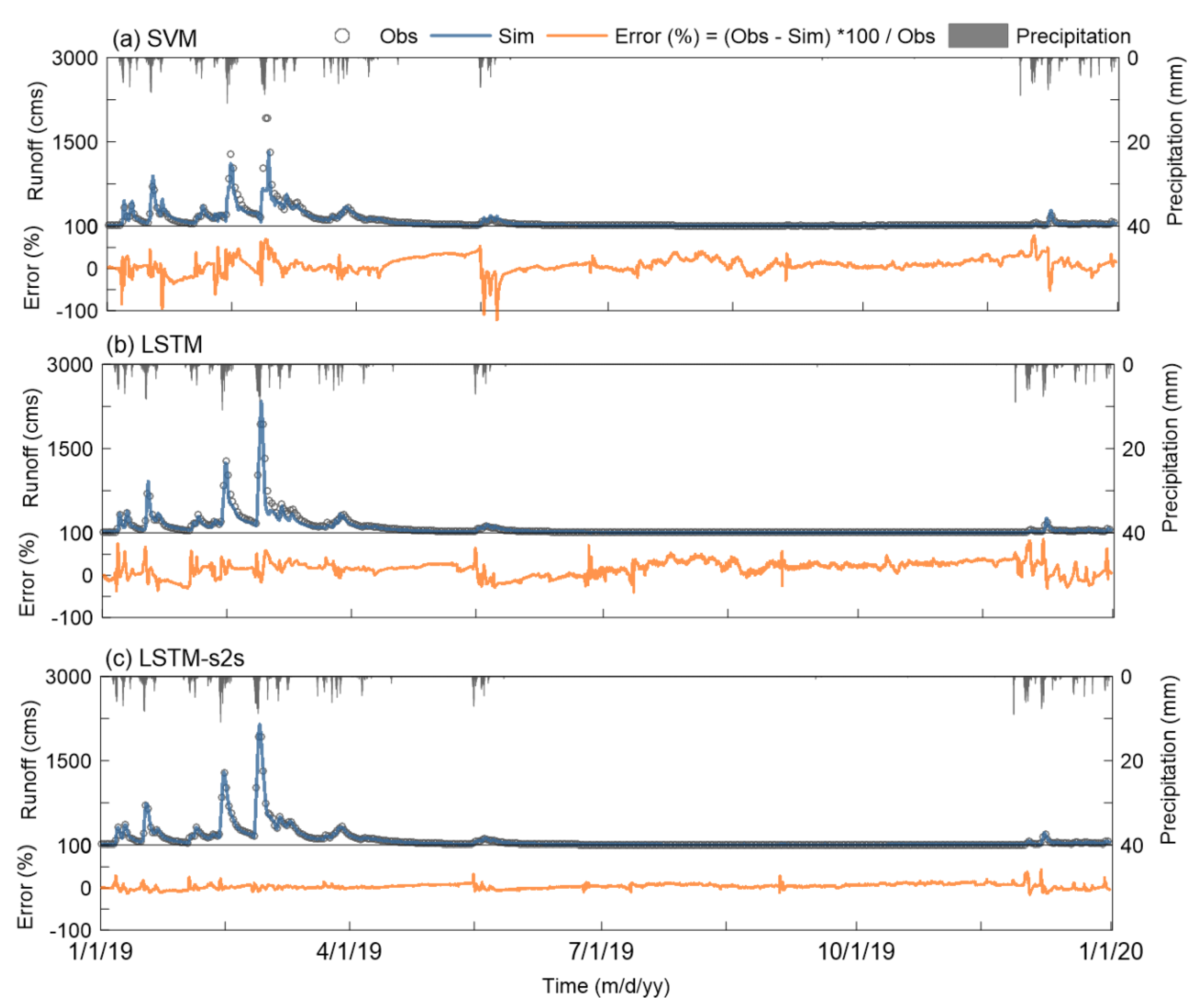
• The LSTM-s2s model outperformed the LSTM and SVM models for 1 to 6 h of lead time. The LSTM-s2s model provided high performance in predicting hourly runoff variability and volume compared to the observed runoff. In addition, the error in simulated runoff was relatively low compared to the other two models. The R² values were over 0.98–0.99 for LSTM-s2s, 0.83–0.86 for LSTM, and 0.68–0.69 for SVM models. The evaluation metrics showed that all three models were suitable for runoff forecasting, but the LSTM-s2s model was the best.
• Seventeen runoff events were separated by three models during the study periods. Similar to the results of overall evaluation, the LSTM-s2s model was the best at predicted runoff events compared to both LSTM and SVM models. The LSTM-s2s model not only showed high performance in predicting peak time and peak runoff value with PRE and PTE values of 3.1% and 1.5 h indicating the predicted runoff event has very low error rates in peak time and value compared to the observations.
• The results of this study represent that machine learning and deep learning approaches such as SVM- and LSTM-based models can be effective alternatives to physics-based hydrological models, which require complex simulation processes for runoff forecasting. Among the three models, the LSTM-s2s model showed the best performance and it was found that this model can be effectively used for hourly runoff forecasting, which is important for developing flood forecasting and warning system.

This study confirmed that the deep learning-based data-driven model provides sufficient potential for runoff forecasting. Obtained results from this study can be used to contribute to improve the ability of short-term flood warning systems. Although runoff forecasting with only 1–6 h of lead time was the focus of this study, it is expected to contribute to various fields, including drought analysis, water resources management for proper irrigation scheduling, and environmental flow analysis based on multiple time-steps from sub-hourly to monthly.

In addition, in this study, even though proposed models used only runoff from upstream areas as input data, new input features such as precipitation, evapotranspiration, snow cover, topography, and geospatial datasets can be used to improve predictive performance in future study. In addition, it was found that the deep learning approach can be applied when it is difficult to use the physics-based hydrological models in regions with temporal and spatial limitations of ground-based observations. The results of this study also represented the strong potential of deep learning-based methods to various hydrological tasks.

References

1. Napolitano, G.; Serinaldi, F.; See, L. Impact of EMD decomposition and random initialisation of weights in ANN hindcasting of daily stream flow series: An empirical examination. J. Hydrol. 2011, 406, 199–214. [Google Scholar] [CrossRef]
2. Young, C.-C.; Liu, W.-C. Prediction and modelling of rainfall–runoff during typhoon events using a physically-based and artificial neural network hybrid model. Hydrol. Sci. J. 2015, 60, 2102–2116. [Google Scholar] [CrossRef]
3. Fan, H.; Jiang, M.; Xu, L.; Zhu, H.; Cheng, J.; Jiang, J. Comparison of Long Short Term Memory Networks and the Hydro-logical Model in Runoff Simulation. Water 2020, 12, 175. [Google Scholar] [CrossRef] [Green Version]
4. Xiang, Z.; Yan, J.; Demir, I. A Rainfall-Runoff Model with LSTM-Based Sequence-to-Sequence Learning. Wat. Resour. Res. 2020, 56. [Google Scholar] [CrossRef]
5. Wu, Z.Y.; Lu, G.H.; Wen, L.; Lin, C.A. Reconstructing and analyzing China’s fifty-nine year (1951–2009) drought history using hydrological model simulation. Hydrol. Earth Syst. Sci. Discuss. 2011, 8, 1861–1893. [Google Scholar]
6. Kang, H.; Sridhar, V. Combined statistical and spatially distributed hydrological model for evaluating future drought indices in Virginia. J. Hydrol. Reg. Stud. 2017, 12, 253–272. [Google Scholar] [CrossRef]
7. Wang, J.; Shi, P.; Jiang, P.; Hu, J.; Qu, S.; Chen, X.; Xiao, Z. Application of BP neural network algorithm in traditional hydrological model for flood forecasting. Water 2017, 9, 48. [Google Scholar] [CrossRef] [Green Version]
8. Hu, C.; Wu, Q.; Li, H.; Jian, S.; Li, N.; Lou, Z. Deep Learning with a Long Short-Term Memory Networks Approach for Rain-fall-Runoff Simulation. Water 2018, 10, 1543. [Google Scholar] [CrossRef] [Green Version]
9. Nash, L.L.; Gleick, P.H. Sensitivity of streamflow in the Colorado Basin to climatic changes. J. Hydrol. 1991, 125, 221–241. [Google Scholar] [CrossRef]
10. Vogel, R.M.; Wilson, I.; Daly, C. Regional Regression Models of Annual Streamflow for the United States. J. Irrig. Drain. Eng. 1999, 125, 148–157. [Google Scholar] [CrossRef]
11. Bicknell, B.R.; Imhoff, J.C.; Kittle, J.L.; Donigian, A.S.; Johanson, R.C. Hydrological Simulation Program-FORTRAN. User’s Manual for Release 11; USEPA: Athens, GA, USA, 1997.
12. Kim, B.K.; Kim, S.D.; Lee, E.T.; Kim, H.S. Methodology for estimating ranges of SWAT model parameters: Application to Imha Lake inflow and suspended sediments. J. Korean Soc. Civ. Eng. 2007, 27, 661–668. [Google Scholar]
13. Neitsch, S.L.; Arnold, J.G.; Kiniry, J.R.; Williams, J.R. Soil and Water Assessment Tool Theoretical Documentation Version 2009; Texas Water Resources Institute Technical Report No. 406; Texas A&M University System: College Station, TX, USA, 2011. [Google Scholar]
14. Devia, G.K.; Ganasri, B.; Dwarakish, G. A Review on Hydrological Models. Aquat. Procedia 2015, 4, 1001–1007. [Google Scholar] [CrossRef]
15. Noh, H.; Lee, J.; Kang, N.; Lee, D.; Kim, H.S.; Kim, S. Long-Term Simulation of Daily Streamflow Using Radar Rainfall and the SWAT Model: A Case Study of the Gamcheon Basin of the Nakdong River, Korea. Adv. Meteorol. 2016, 2016, 1–12. [Google Scholar] [CrossRef]
16. Mosavi, A.; Ozturk, P.; Chau, K.-W. Flood Prediction Using Machine Learning Models: Literature Review. Water 2018, 10, 1536. [Google Scholar] [CrossRef] [Green Version]
17. McCulloch, W.S.; Pitts, W. A logical calculus of the ideas immanent in nervous activity. Bull. Math. Biol. 1943, 5, 115–133. [Google Scholar] [CrossRef]
18. Vapnik, V. The Nature of Statistical Learning Theory; Springer: New York, NY, USA, 1995. [Google Scholar]
19. Breiman, L.; Friedman, J.H.; Olshen, R.A.; Stone, C.J. Classification and Regression Trees; Chapman and Hall/CRC: Boca Raton, FL, USA, 1984. [Google Scholar]
20. LeCun, Y.; Haffner, P.; Bottou, L.; Bengio, Y. Object Recognition with Gradient-Based Learning. In Shape, Contour and Grouping in Computer Vision; Lecture Notes in Computer Science; Springer: Berlin/Heidelberg, Germany, 1999; Volume 1681, pp. 319–345. [Google Scholar] [CrossRef]
21. Rumelhart, D.E.; Hinton, G.E.; Williams, R.J. Learning representations by back-propagating errors. Nat. Cell Biol. 1986, 323, 533–536. [Google Scholar] [CrossRef]
22. Hochreiter, S.; Schmidhuber, J. Long Short-Term Memory. Neural Comput. 1997, 9, 1735–1780. [Google Scholar] [CrossRef]
23. Feng, D.; Fangi, D.K.; Shen, C. Enhancing Streamflow Forecast and Extracting Insights Using Long-Short Term Memory Networks With Data Integration at Continental Scales. Water Resour. Res. 2020, 56, 026793. [Google Scholar] [CrossRef]
24. Solomatine, D.P.; Ostfeld, A. Data-driven modelling: Some past experiences and new approaches. J. Hydroinformatics 2008, 10, 3–22. [Google Scholar] [CrossRef] [Green Version]
25. Solomatine, D.P.; Dulal, K.N. Model trees as an alternative to neural networks in rainfall—Runoff modelling. Hydrol. Sci. J. 2003, 48, 399–411. [Google Scholar] [CrossRef]
26. Jothiprakash, V.; Magar, R. Multi-time-step ahead daily and hourly intermittent reservoir inflow prediction by artificial intelligent techniques using lumped and distributed data. J. Hydrol. 2012, 2012, 293–307. [Google Scholar] [CrossRef]
27. Lin, G.-F.; Jhong, B.-C.; Chang, C.-C. Development of an effective data-driven model for hourly typhoon rainfall forecasting. J. Hydrol. 2013, 495, 52–63. [Google Scholar] [CrossRef]
28. Ba, H.; Guo, S.; Wang, Y.; Hong, X.; Zhong, Y.; Liu, Z. Improving ANN model performance in runoff forecasting by adding soil moisture input and using data preprocessing techniques. Hydrol. Res. 2018, 49, 744–760. [Google Scholar] [CrossRef] [Green Version]
29. Chang, F.-J.; Tsai, M.-J. A nonlinear spatio-temporal lumping of radar rainfall for modeling multi-step-ahead inflow forecasts by data-driven techniques. J. Hydrol. 2016, 535, 256–269. [Google Scholar] [CrossRef]
30. Bui, D.T.; Hoang, N.D.; Martínez-Álvarez, F.; Ngo, P.T.T.; Hoa, P.V.; Pham, T.D.; Costache, R. A novel deep learning neural network approach for predicting flash flood susceptibility: A case study at a high frequency tropical storm area. Sci. Total Environ. 2020, 701, 134413. [Google Scholar]
31. Feng, Y.; Cui, N.; Hao, W.; Gao, L.; Gong, D. Estimation of soil temperature from meteorological data using different ma-chine learning models. Geoderma 2019, 338, 67–77. [Google Scholar] [CrossRef]
32. Tayfur, G.; Singh, V.P. ANN and Fuzzy Logic Models for Simulating Event-Based Rainfall-Runoff. J. Hydraul. Eng. 2006, 132, 1321–1330. [Google Scholar] [CrossRef] [Green Version]
33. Behzad, M.; Asghari, K.; Eazi, M.; Palhang, M. Generalization performance of support vector machines and neural networks in runoff modeling. Expert Syst. Appl. 2009, 36, 7624–7629. [Google Scholar] [CrossRef]
34. Ghumman, A.R.; Ghazaw, Y.M.; Sohail, A.; Watanabe, K. Runoff forecasting by artificial neural network and conventional model. Alex. Eng. J. 2011, 50, 345–350. [Google Scholar] [CrossRef] [Green Version]
35. Muñoz, P.; Orellana-Alvear, J.; Willems, P.; Célleri, R. Flash-Flood Forecasting in an Andean Mountain Catch-ment—Development of a Step-Wise Methodology Based on the Random Forest Algorithm. Water 2018, 10, 1519. [Google Scholar] [CrossRef] [Green Version]
36. Venkatesan, E.; Mahindrakar, A.B. Forecasting floods using extreme gradient boosting-a new approach. Int. J. Civ. Eng. Tech. 2019, 10, 1336–1346. [Google Scholar]
37. Bae, Y.; Kim, J.; Wang, W.; Yoo, Y.; Jung, J.; Kim, H.S. Monthly Inflow Forecasting of Soyang River Dam Using VARMA and Machine Learning Models. J. Clim. Res. 2019, 14, 183–198. [Google Scholar] [CrossRef]
38. Assem, H.; Gharbia, S.S.; Makrai, G.; Johnston, P.; Gill, L.; Pilla, F. Urban Water Flow and Water Level Prediction Based on Deep Learning. In Joint European Conference on Machine Learning and Knowledge Discovery in Databases; Lecture Notes in Computer Science; Springer Nature: Skopje, Macedonia, 18–22 September 2017; pp. 317–329. [Google Scholar]
39. Park, M.K.; Yoon, Y.S.; Lee, H.H.; Kim, J.H. Application of recurrent neural network for inflow prediction into multi-purpose dam basin. J. Korea Water Res. Assoc. 2018, 51, 1217–1227. [Google Scholar]
40. Kratzert, F.; Klotz, D.; Brenner, C.; Schulz, K.; Herrnegger, M. Rainfall–runoff modelling using Long Short-Term Memory (LSTM) networks. Hydrol. Earth Syst. Sci. 2018, 22, 6005–6022. [Google Scholar] [CrossRef] [Green Version]
41. Mok, J.Y.; Choi, J.H.; Moon, Y.I. Prediction of multipurpose dam inflow using deep learning. J. Korea Water Res. Assoc. 2020, 53, 97–105. [Google Scholar]
42. Van, S.P.; Le, H.M.; Thanh, D.V.; Dang, T.D.; Loc, H.H.; Anh, D.T. Deep learning convolutional neural network in rain-fall-runoff modelling. J. Hydroinf. 2020, 22, 541–561. [Google Scholar] [CrossRef]
43. Cho, K.; Van Merrienboer, B.; Bahdanau, D.; Bengio, Y. On the Properties of Neural Machine Translation: Encoder–Decoder Approaches. In Proceedings of the SSST-8, Eighth Workshop on Syntax, Semantics and Structure in Statistical Translation, Doha, Qatar, 25 October 2014. [Google Scholar]
44. Sutskever, I.; Vinyals, O.; Le, Q.V. Sequence to sequence learning with neural networks. Adv. Neural Inf. Process. Syst. 2014, 2, 3104–3112. [Google Scholar]
45. Johnson, L.E.; Hsu, C.; Zamora, R.; Cifelli, R. Assessment and Applications of Distributed Hydrologic Model-Russian-Napa River Basins, CA; NOAA Technical Memorandum PSD-316; NOAA Printing Office: Silver Spring, MD, USA, 2016.
46. Han, H.; Kim, J.; Chandrasekar, V.; Choi, J.; Lim, S. Modeling Streamflow Enhanced by Precipitation from Atmospheric River Using the NOAA National Water Model: A Case Study of the Russian River Basin for February 2004. Atmosphere 2019, 10, 466. [Google Scholar] [CrossRef] [Green Version]
47. Gholami, V.; Chau, K.W.; Fadaee, F.; Torkaman, J.; Ghaffari, A. Modeling of groundwater level fluctuations using dendro-chronology in alluvial aquifers. J. Hydrol. 2015, 529, 1060–1069. [Google Scholar] [CrossRef]
48. Choi, C.; Kim, J.; Han, H.; Han, D.; Kim, H.S. Development of Water Level Prediction Models Using Machine Learning in Wetlands: A Case Study of Upo Wetland in South Korea. Water 2019, 12, 93. [Google Scholar] [CrossRef] [Green Version]
49. Drucker, H.; Burges, C.J.; Kaufman, L.; Smola, A.J.; Vapnik, V. Support vector regression machines. In Advances in Neural Information Processing Systems; MIT Press: Cambridge, MA, USA, 1996. [Google Scholar]
Figure 1. The Russian River basin, California. Orange points represent five runoff stations located in the basin.
Water 13 00437 g001
Figure 2. Conceptual diagram of the long short-term memory (LSTM) model.
Water 13 00437 g002
Figure 3. Conceptual diagram of LSTM with the sequence-to-sequence structure model.
Water 13 00437 g003
Figure 4. Observed and predicted runoff and errors with lead time of 1 h from three data-driven models. (ac) indicate the results of SVM, LSTM, and LSTM-s2s models.
Water 13 00437 g004
Figure 5. Comparison results of predicted runoff with observations for lead time of (a) 1 h and (b) 6 h. Red line indicates regression line of two runoff data.
Water 13 00437 g005
Figure 6. Statistical metrics with lead times from 1 to 6 h. (a) and (b) show the results of RMSE and NSE.
Water 13 00437 g006
Figure 7. Event-based evaluation results from SVM, LSTM, and LSTM-s2s models. (af) represent the six events provided from observation and three models.
Water 13 00437 g007
Figure 8. Scatter plots showing the performance of the LSTM-s2s model compared to other models for event-based runoff prediction using four metrics. (ad) indicate four metrics, R2, RMSE, PRE, and PTE.
Water 13 00437 g008