A Simple Method for the Control Time of a Pumping Station to Ensure a Stable Water Level Immediately Upstream of the Pumping Station under a Change of the Discharge in an Open Channel

Abstract

For an open channel with cascade pumping stations, the water level immediately upstream of the pumping station should be kept constant to ensure pumping stability and lining safety. In this study, a simple method was proposed to determine the control time of the pumping station to ensure a stable water level immediately upstream of the pumping station using reverse analysis. The variable discharge process and fixed water level were taken as the upstream and downstream boundaries of the one-dimensional open channel hydrodynamic model, and the discharge process of the pumping station was obtained under ideal conditions. The control time was determined by the equivalent water volume change considering the step change of the discharge of the pumping station. A case study was performed using the Jiaodong water diversion project from Songzhuang sluice to Huibu pumping station (G1–P1), and the effects of the initial discharge, variable discharge, and downstream water level on the control time were investigated. The results show that (1) the larger the initial discharge, the shorter the control time; (2) increasing the upstream discharge reduced the control time, while decreasing the upstream discharge increased the control time; (3) the control time decreased with the increase of the water depth immediately upstream of the pumping station.

1. Introduction

There is a sharp contradiction between the supply and demand of water resources in many countries because of their uneven spatial and temporal distributions [1,2,3]. Numerous open channels with cascade pumping stations have been constructed as a solution to this problem [4,5,6]. However, improper control of these cascade pumping stations may cause channel overflow, drying up of the pumping station forebay, low pumping efficiency, and even some catastrophic events, such as pumping unit vibration and channel lining damage. More importantly, as the energy consumption and operation cost of the pumping station is very high, a number of studies have been conducted on energy savings [7,8,9,10,11,12,13,14] and economic operations [15,16,17,18] of a pumping station. Liu et al. [19] proposed an improved self-adaptive grey wolf optimizer (IAGWO) to minimize the total daily cost and maximize the efficiency of cascade pumping stations, and as a result, 0.80268% of the daily operating cost could be saved. Zhuan et al. [20] proposed a decomposition method that is capable of reducing the dimensionality of the optimization problem, and the energy cost was reduced by 2.54% compared with the benchmark scheduling. Zhang et al. [12] proposed a scheduling optimization method based on station skipping, in which one or more pumping stations could be reduced and the allocation of a gross head to other stations was optimized. Gong and Chen [21] proposed an optimization model of cascade pumping stations by considering water level requirements.

However, it is noted that these studies have focused mainly on the economic operations and energy savings of cascade pumping stations under steady-state conditions without considering their safety during the switching of working conditions. Some automatic control algorithms, including feedforward control (e.g., Saint Venant equations inversion method [22] and the volume compensation (VC) method [23]) and feedback control (e.g., proportional–integral–derivative (PID) control [24], linear quadratic regulator (LQR) [25], and model predictive control (MPC) [26]), have been proposed to deal with such situations. Wahlin et al. [27] found that combined feedforward–feedback controllers were better than either feedforward or feedback controllers alone. Kong et al. [28] added a deviation weight coefficient into the algorithm for the middle route of the South-to-North Water Diversion Project, which could keep the water level deviations in all pools to certain proportions. However, these automatic control algorithms are incapable of dealing with the switching of working conditions and are rarely used in pumping stations.

Some scholars have studied the real-time control of drainage pumping stations. Studies have shown that real-time control is a reliable and cost-effective solution that improves the performance of urban drainage systems [29]. Chang et al. [30] proposed the counterpropagation fuzzy-neural network for extracting flood control knowledge in the form of fuzzy if–then rules and applied it to the Yu-Cheng pumping station in Taipei City. The results indicated the model had the potential to automatically control the system in real time. Hsu et al. [31] used an adaptive network-based fuzzy information system to build two real-time pumping station operation models based on the historical operation records (ANFIS-His) and the best operation series (ANFIS-Opt), and the result showed ANFIS-Opt was better than ANFIS-His for the drainage system in New Taipei city. Mullapudi et al. [32] formulated a reinforcement learning (RL) algorithm for the real-time control of urban stormwater systems, where the results indicated that RL could effectively control individual sites in an urban watershed in Ann Arbor. Pereira et al. [33] designed a PID controller to automate the operation of the Lordelo pumping station based on the intake water level measurements. The result showed that the automation is close to the manual procedures.

Few scholars have studied the hydraulic control of water supply pumping stations. Eker and Kara [34] developed an optimization algorithm for water level control by adjusting the pump speed. Abdulrahman and Nasher [35] used a model predictive controller to maintain a stable flow and reduce the operation cost by manipulating the pump speed. However, these algorithms are very complex and time-consuming, making them impractical for real engineering applications. The control of pumping stations can be considered as a problem of determining the startup and shutdown times of pump units. Wu et al. [36] proposed formulas for calculating the opening time of the pumping station, the increasing rate of the water level, and the water level. Gao et al. [37] simulated changes in water level immediately upstream of the pumping station under different conditions and determined the difference in opening times of adjacent pumping stations (the difference between the start-up times of the previous and next cascade pumping stations). However, the stability of the water level immediately upstream of the pumping station is often ignored. In view of this, a simple and rapid method was proposed to determine the control time of the pumping station to ensure the stability of the water level immediately upstream of the pumping station using reverse analysis, and the effects of initial discharge, variable discharge, and water level immediately upstream of the pumping station on the control time were analyzed.

The rest of this paper is structured as follows. Section 2 introduces the one-dimensional hydrodynamic model and its solution; Section 3 describes the method for determining the control time of the pumping station; Section 4 applies the method to the Jiaodong Water Diversion Project and analyzes the effects of the initial discharge, variable discharge, and water level immediately upstream of the pumping station on the control time; Section 5 presents the conclusions.

2. One-Dimensional Hydrodynamic Model

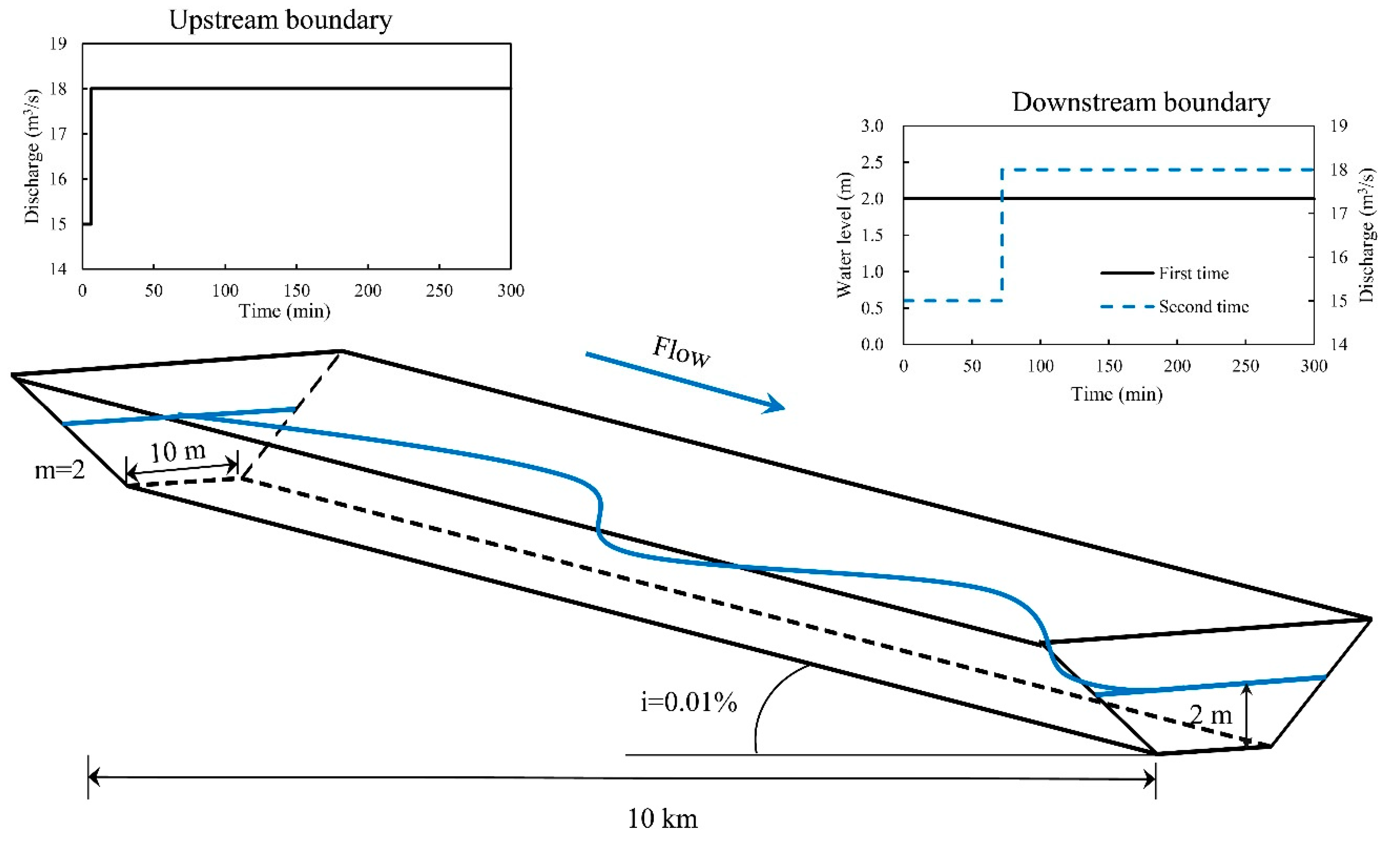
2.1. Open Channel

The governing equations for the one-dimensional unsteady flow in an open channel were first proposed by Saint Venant in 1871, including continuity and momentum equations [38]:

$$B\frac{\partial Z}{\partial t}+\frac{\partial Q}{\partial x}=q,$$

(1)

$$\frac{\partial Q}{\partial t}+\frac{\partial }{\partial x}\left(\frac{\alpha Q^2}{A}\right)+gA\frac{\partial Z}{\partial x}+gA{S}_f=0,$$

(2)

where B is the channel surface width (m); Z is the water level (m); t is the time (s); Q is the discharge (m³/s); x is the distance along the channel (m); q is the lateral inflow (m³/s); α is the momentum correction coefficient, A is the wetted cross-sectional area (m²); g is the gravitational acceleration (m/s²); and S_f is the friction slope, which can be expressed as follows:

$$S_f=\frac{n^{2}Q\left|Q\right|}{A^2{R}^{4/3}},$$

(3)

where n is the Manning’s roughness coefficient and R is the hydraulic radius of the channel (m).

2.2. Water Conveyance Structure

An inverted siphon is a common water conveyance structure with quite different hydraulic characteristics from that of an open channel such that the Saint Venant equations are not applicable to an inverted siphon and must be modified. In this study, the ratio of the sectional area of the inverted siphon to that of the adjacent channel is greater than 0.5, indicating that inverted siphon has little effect on the flow. As the inverted siphon is less than 500 m long and the propagation speed of the water hammer in the pipeline is about 1000 m/s, the propagation time is less than 0.5 s. The computational time step of the open channel is 120 s, which is much longer than the propagation time of flow in the inverted siphon. Therefore, the inverted siphon can be treated as head loss [39]. The continuity and energy equations are used as the governing equations, which are solved simultaneously using the Saint Venant equations. The control equations of the inverted siphon are described as follows:

$$Q_{in}=Q_{out},$$

(4)

$$Z_{in}=Z_{out}+\left(\frac{2g{n}_{is}^2{L}_{is}}{R_{is}^{4/3}}+{\xi }_{is}\right)\frac{Q_{out}^2}{2g{A}_{is}},$$

(5)

where Q_in and Q_out are the inlet and outlet discharges of the inverted siphon (m³/s); Z_in and Z_out are the inlet and outlet water levels of the inverted siphon (m); n_is is the roughness of the inverted siphon; L_is is the length of the inverted siphon (m); R_is is the hydraulic radius (m); ξ_is is the local loss coefficient of the inverted siphon; A_is is the wetted cross-sectional area of the inverted siphon (m²).

The discharge process is set as the outer boundary, which is equivalent to the separate calculation of two sections of the channel. The discharge of the pumping station is assigned according to the actual change in discharge.

The Preissmann four-point implicit difference method was used to discretize the Saint Venant equations due to its advantages of fast convergence, high efficiency, and good stability [40], and the chasing method was used to solve the discrete equation [41]. See [6] for detailed steps.

3. Determination of the Control Time of the Pumping Station

3.1. Theoretical Basis

For an open channel with cascade pumping stations, the water levels immediately upstream of the pumping stations should be kept stable as much as possible in order to ensure the safety of the pumping station and reduce the damage to the canal lining. When the upstream discharge of the channel changes, the control times of pump units need to be determined according to changes in the discharge immediately upstream of the pumping station. In this study, reverse analysis was used to calculate the discharge immediately upstream of the pumping station in response to changes in upstream discharge and the water level immediately upstream of the pumping station was assumed to be fixed. However, discharge cannot be regulated according to the ideal discharge process in actual projects according to the characteristics of step-by-step or sudden changes, which means that the pump instantaneously changes from the earlier rate to the new pumping rate. Therefore, the single-step change process, which is closest to the actual control process of the pumping station, was considered for simplicity. Because the discharge is less affected by the head, the influence of the head on discharge was not considered. As shown in Figure 1, t₂ is the control time of the pumping station, which can be determined as follows:

(1)

An initial stable and non-uniform flow was assumed for the open channel.

(2)

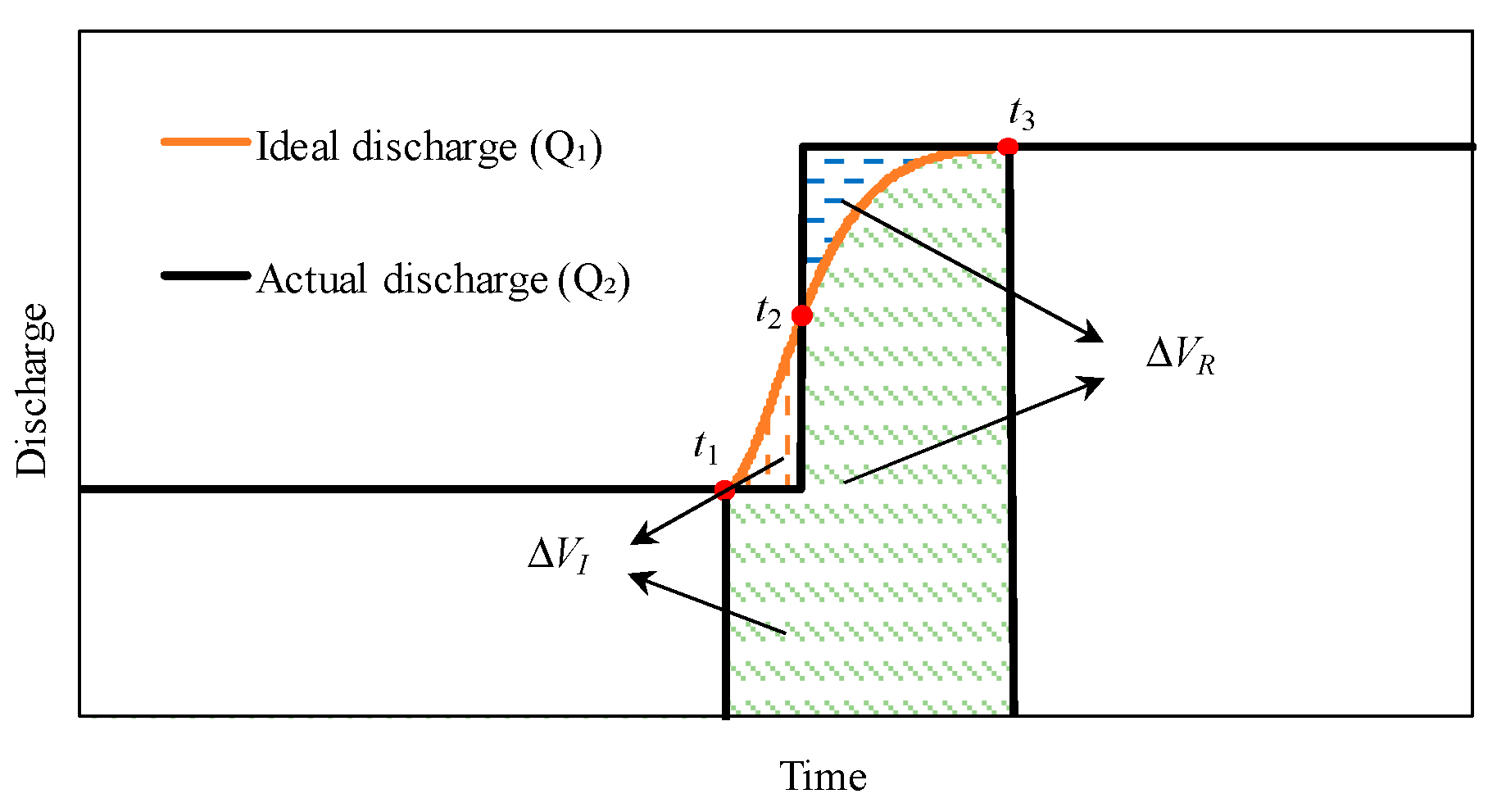
The initial arrival time of the flow to the pumping station (t₁) was determined when the discharge immediately upstream of the pumping station was increased by 1% of the variable discharge.

(3)

The complete arrival time of the flow to the pumping station (t₃) was determined when the discharge immediately upstream of the pumping station was increased by 99% of the variable discharge.

(4)

The control time of the pumping station (t₂): As the forebay of the pumping station has some storage capacity and the upstream flow is not affected by the pumping station, the same pumping volume in the same period will result in the same water level variation. Under ideal conditions, the ideal pumping volume ΔV_I of the pumping station in the period of t₁–t₃ can be expressed as follows:

$$\Delta V_I={\displaystyle {\int }_{t_1}^{t_3}{Q}_1\left(t\right)}dt.$$

(6)

The actual pumping volume ΔV_R in the period of t₁–t₃ can be expressed as follows:

$$\Delta V_R={\displaystyle {\int }_{t_1}^{t_3}{Q}_2\left(t\right)}dt.$$

(7)

Considering the characteristics of the step change of discharge, the control time (t₂) is the time when the actual pumping volume is equal to the ideal pumping volume in the period of t₁–t₃:

$$\Delta V_I=\Delta V_R,$$

(8)

$${\displaystyle {\int }_{t_1}^{t_2}{Q}_1\left(t\right)-Q_2\left(t\right)}dt={\displaystyle {\int }_{t_2}^{t_3}{Q}_2\left(t\right)-Q_1\left(t\right)}dt.$$

(9)

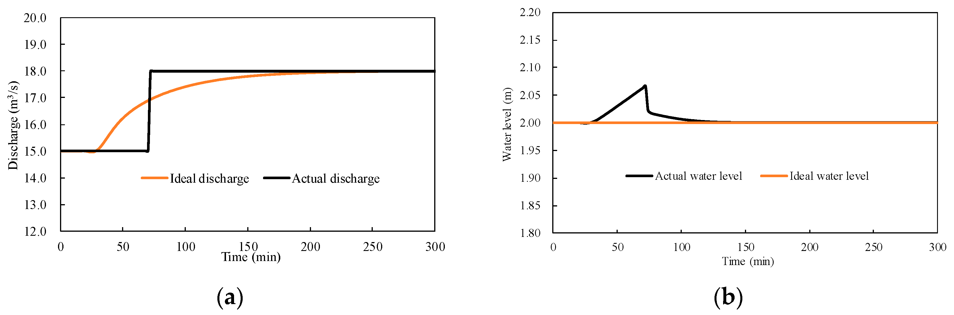
3.2. Experimental Verification

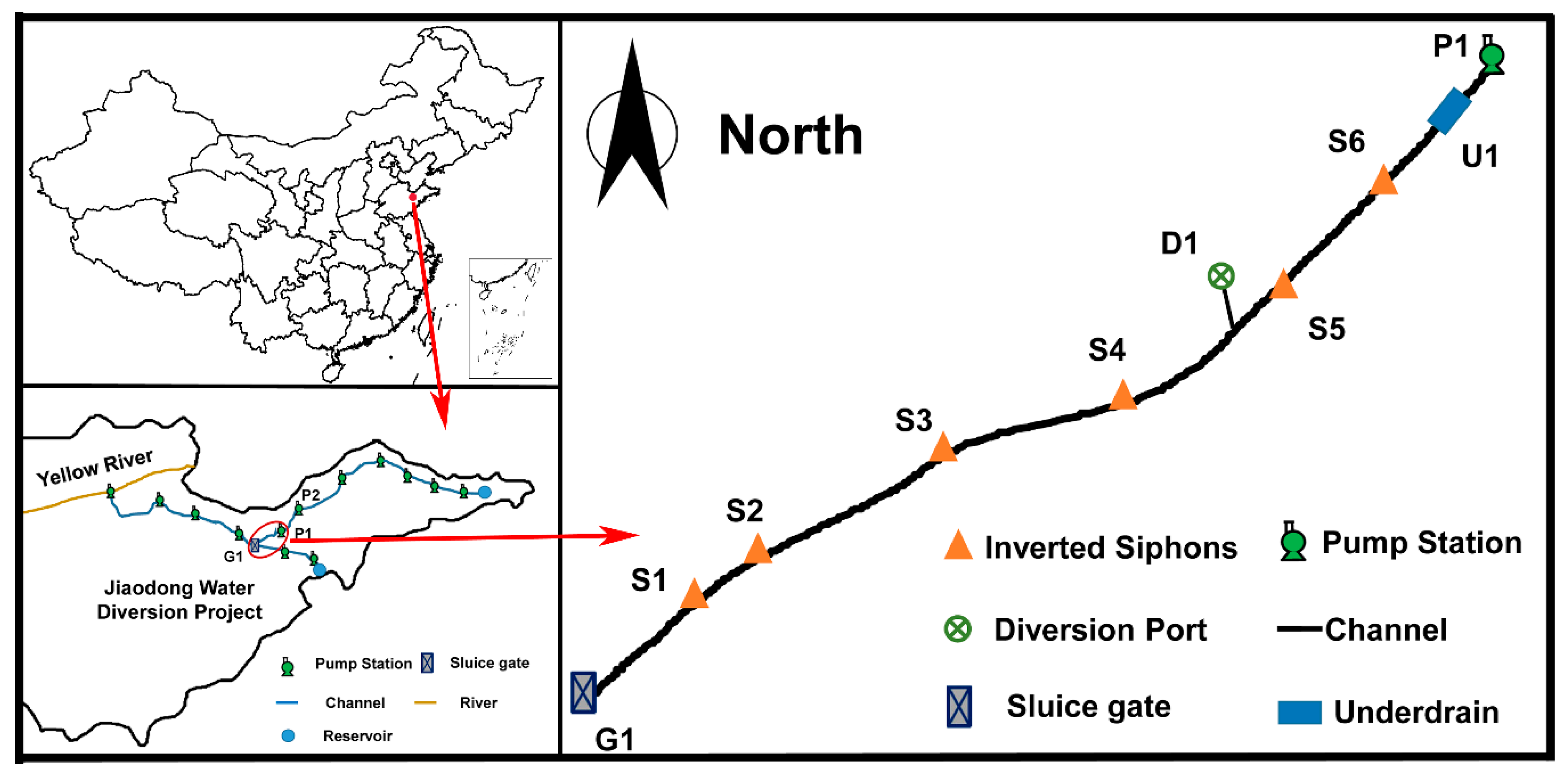
As is shown in Figure 2, the hydrodynamic model was verified with a 10.00 km long trapezoidal channel with a bottom width of 10.00 m, a downstream bottom elevation of 0 m, a side slope coefficient of m = 2, a bottom slope of i = 0.01%, and a roughness of 0.015.

The upstream boundary discharge was 15.0 m³/s, the downstream boundary water level was 2.00 m, and the variable discharge was 3.0 m³/s. The calculated downstream discharge variation is shown in Figure 3a. The initial arrival time of the variable discharge (t₁) was 30 min, the complete arrival time (t₃) was 244 min, and the control time (t₂) was 72 min. Assuming that the upstream boundary remained unchanged and the downstream boundary was set as the discharge of the pumping station, the downstream water level was calculated. Figure 3b shows that the downstream water level returned to the original water level of 2.00 m after a short period of fluctuation, indicating that a reliable control time can be obtained for the pumping station. In this study, the pumping rate was assumed to be changed instantaneously. However, the changing time of the discharge may vary between different pumping stations, which can have an effect on the control time. At changing times of 0 min, 10 min, and 20 min, the control times were calculated to be 72 min, 68 min, and 64 min, respectively. Thus, the control time decreased as the changing time increased. This was because the discharge of the pumping station was lower than that under stable flow conditions (18 m³/s) and it needed to be adjusted earlier. However, for the sake of simplicity, the influence of the discharge changing time was not considered in the next sections.

4. Case Study

The Jiaodong Water Diversion Project is located in the Shandong Province, China, which has supplied 2.515 billion m³ water to the Jiaodong area and thus plays a critical role in the social and economic development of the area. The project is about 570 km long with 13 pumping stations and more than 60 inverted siphons. The section from the Songzhuang sluice to the Huibu pumping station (G1–P1) was selected as the case study, where the total length is 35.83 km, the bottom width is 4.50–8.20 m, the side slope coefficient is 2, and the bottom slope is 0.05–0.10%. The design water level immediately upstream of the pumping station is 4.52 m, the design water depth is 2.42 m, and the design discharge of G1 is 22 m³/s. There are six inverted siphons, one diversion port, and one underdrain in G1–P1 (Figure 4). The parameters of the inverted siphons are shown in

Table 1. The parameters of inverted siphons.

Name	Length (m)	Number of Holes	Width (m)	Height (m)	Area (m2)	Area of Upstream Open Channel (m2)	Area Ratio	Area of Downstream Open Channel (m2)	Area Ratio
S1	94	2	2.5	2.5	12.5	25	0.5	25	0.5
S2	421	2	3	3	18	25	0.72	33	0.55
S3	85.5	2	3	3	18	33	0.55	33	0.55
S4	161	2	3	3	18	33	0.55	33	0.55
S5	235	2	3	3	18	31.25	0.58	23.75	0.76
S6	447	2	3	3	18	23.75	0.76	23.75	0.76

.

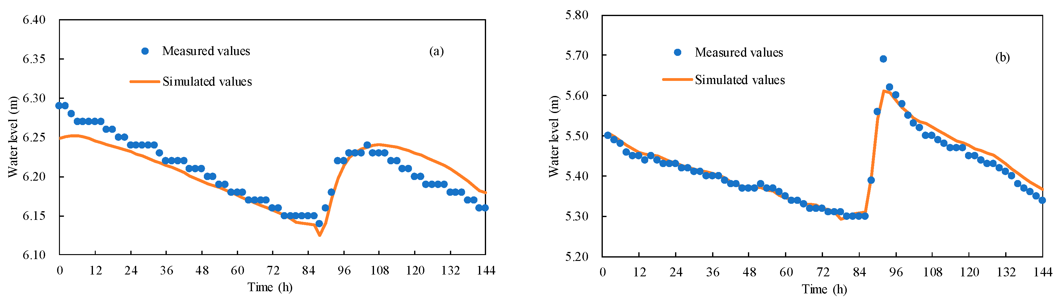
4.1. Verification of the Hydrodynamic Model

The hydrodynamic model of G1–P1 was established and verified using the measured data from 16 May 2018 to 21 May 2018. The measured and simulated water levels at the inlets of Shuangshan river inverted siphon (S5) and Ze river inverted siphon (S6) were analyzed and compared using the maximum and average errors as the evaluation criteria. Figure 5 shows that the maximum and average errors of the water levels at the S5 inlet were 0.04 m and 0.01 m, while those at the S6 inlet were 0.08 m and 0.01 m, respectively. Thus, there was only a marginal difference between the simulated and measured water levels, and thus, the proposed hydrodynamic model could be used to simulate the hydrodynamics of the Jiaodong Water Diversion Project.

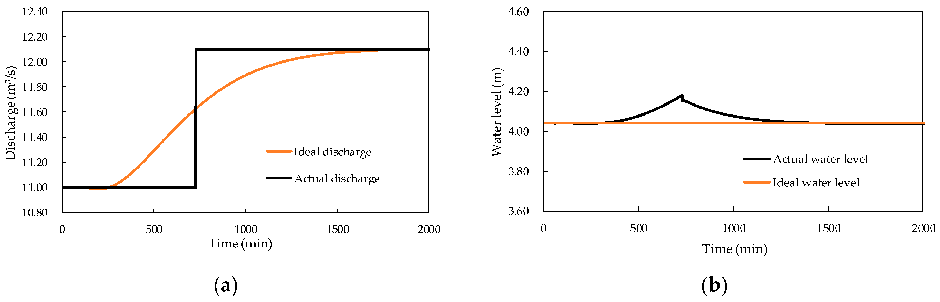
4.2. Verification of the Control Time of the Pumping Station

Here, G1–P1 is used as an example to verify the reliability of the proposed method. The upstream boundary discharge was 11.0 m³/s (50% of the design discharge), the downstream boundary water level was 4.04 m (80% of the design water depth), and the variable discharge was 1.1 m³/s (5% of the design discharge). The calculated downstream discharge variation is shown in Figure 6a. The initial arrival time of the variable discharge (t₁) was 276 min, the complete arrival time (t₃) was 1668 min, and the control time (t₂) was 728 min. Assuming that the upstream boundary remained unchanged and the downstream boundary was set as the discharge of the pumping station, the downstream water level was calculated. Figure 6b shows that the water level immediately upstream of P1 returned to the original water level of 4.04 m after a short period of fluctuation, indicating that a reliable control time could be obtained for the pumping station in this case study.

4.3. Factors Affecting the Control Time of the Pumping Station

The control time of the pumping station is closely related to the propagation time of the flow, which in turn is affected by the channel length and roughness, initial discharge, variable discharge, and water depth immediately upstream of the pumping station. As the channel length and roughness are constant in G1–P1, the effects of other factors on the control time of the pumping station were analyzed in this study.

4.3.1. Effects of the Initial Discharge

Five initial discharges (30%, 40%, 50%, 60%, and 70% of the design discharge) and one water level immediately upstream of the pumping station (4.04 m, 80% of the design water depth) were set according to the actual operation of G1–P1. The control time of P1 (t) was calculated when the discharge at G1 was increased or decreased by 1.1 m³/s (10% of the design discharge). The design discharge was taken as the base discharge (Q₀) and the time obtained by dividing the channel length by the design flow velocity was taken as the base time (t₀). The calculation results are dimensionless and shown in Figure 7.

Figure 7 shows that as the upstream discharge was increased by 1.1 m³/s, t/t₀ reached a maximum at an initial discharge of 6.6 m³/s (30% of the design discharge) and a minimum at an initial discharge of 15.4 m³/s (70% of the design discharge). As Q/Q₀ increased, t/t₀ gradually decreased. The fitting results show that there was a power function relationship between Q/Q₀ and t/t₀. Similar results were obtained as the upstream discharge was decreased by 1.1 m³/s. Thus, it was concluded that the control time decreased with the increase of the initial discharge at a constant variable discharge.

The propagation velocity of an unsteady flow is related to the wave velocity and flow velocity [42]. In this study, the upstream discharge changed and the wave propagation direction was consistent with the flow direction, and thus, the propagation velocity was the sum of wave velocity and flow velocity [43]. The wave velocity is mainly affected by the average water depth, and the greater the average water depth is, the greater the wave velocity will be, while the flow velocity is mainly affected by the discharge and wetted cross-sectional area, and the larger the discharge is and the smaller the wetted cross-sectional area is, the greater the flow velocity will be. The cross-sections at both ends of G1–P1 (G1–S1 and U1–P1) were selected for analysis and the flow velocity and wave velocity at different initial discharges were calculated.

Table 2. Hydraulic parameters under different initial discharges.

Initial Discharge (m3/s)	Channel Section		Water Depth (m)	Wetted Cross-Sectional Area (m2)	Flow Velocity (m/s)	Wave Velocity (m/s)	Propagation Velocity (m/s)
6.6	Downstream of G1	Before change	1.46	11.53	0.57	3.78	4.35
		After change	1.60	13.10	0.59	3.96	4.55
	Upstream of S1	Before change	1.79	15.39	0.43	4.19	4.62
		After change	1.94	17.19	0.45	4.36	4.81
	Downstream of U1	Before change	1.68	14.05	0.47	4.06	4.53
		After change	1.69	14.21	0.54	4.08	4.62
	Upstream of P1	Before change	1.94	17.23	0.38	4.36	4.74
		After change	1.94	17.23	0.45	4.36	4.81
8.8	Downstream of G1	Before change	1.73	14.65	0.60	4.12	4.72
		After change	1.86	16.17	0.61	4.27	4.88
	Upstream of S1	Before change	2.07	18.96	0.46	4.51	4.97
		After change	2.20	20.69	0.48	4.65	5.13
	Downstream of U1	Before change	1.71	14.40	0.61	4.10	4.71
		After change	1.73	14.60	0.68	4.12	4.80
	Upstream of P1	Before change	1.94	17.23	0.51	4.36	4.87
		After change	1.94	17.23	0.57	4.36	4.93
11	Downstream of G1	Before change	1.98	17.68	0.62	4.40	5.02
		After change	2.09	19.18	0.63	4.52	5.16
	Upstream of S1	Before change	2.32	22.40	0.49	4.77	5.26
		After change	2.44	24.09	0.50	4.89	5.39
	Downstream of U1	Before change	1.75	14.82	0.74	4.14	4.88
		After change	1.76	15.05	0.80	4.16	4.96
	Upstream of P1	Before change	1.94	17.23	0.64	4.36	5.00
		Before change	1.94	17.23	0.70	4.36	5.06
13.2	Downstream of G1	Before change	2.20	20.67	0.64	4.64	5.28
		After change	2.30	22.15	0.65	4.75	5.40
	Upstream of S1	Before change	2.55	25.77	0.51	5.00	5.51
		After change	2.66	27.43	0.52	5.11	5.63
	Downstream of U1	Before change	1.79	15.31	0.86	4.19	5.05
		After change	1.81	15.57	0.92	4.21	5.13
	Upstream of P1	Before change	1.94	17.23	0.77	4.36	5.13
		Before change	1.94	17.23	0.83	4.36	5.19
15.4	Downstream of G1	Before change	2.41	23.62	0.65	4.86	5.51
		After change	2.51	25.09	0.66	4.96	5.62
	Upstream of S1	Before change	2.76	29.08	0.53	5.21	5.74
		After change	2.86	30.72	0.54	5.30	5.84
	Downstream of U1	Before change	1.83	15.86	0.97	4.24	5.21
		After change	1.85	16.15	1.02	4.27	5.29
	Upstream of P1	Before change	1.94	17.23	0.89	4.36	5.25
		Before change	1.94	17.23	0.96	4.36	5.32

shows that with the increase of the initial discharge, the water depth and wetted cross-sectional area at each section (except the last section) increased, resulting in an increase in the wave velocity. Although the wetted cross-sectional area was inversely proportional to flow velocity, the increase of the discharge led to an increase in flow velocity. Therefore, the control time of the pumping station decreased with the increase in the initial discharge. Because the channel is trapezoid-shaped, the water depth increased and the wave velocity decreased with the increase of the initial discharge. In addition, because the increasing rate of discharge was lower than that of wetted cross-sectional area, the increase in the flow velocity also decreased. Therefore, the increase of propagation velocity and the decrease of the control time decreased with the increase in the initial discharge. It is seen from Table 2 that there was a power relationship between the average propagation velocity and the initial discharge (v = 3.1818 × Q^0.1973, R² = 0.9984). Because the control time is proportional to the reciprocal of the average propagation velocity, the control time and the initial discharge were in a power relationship.

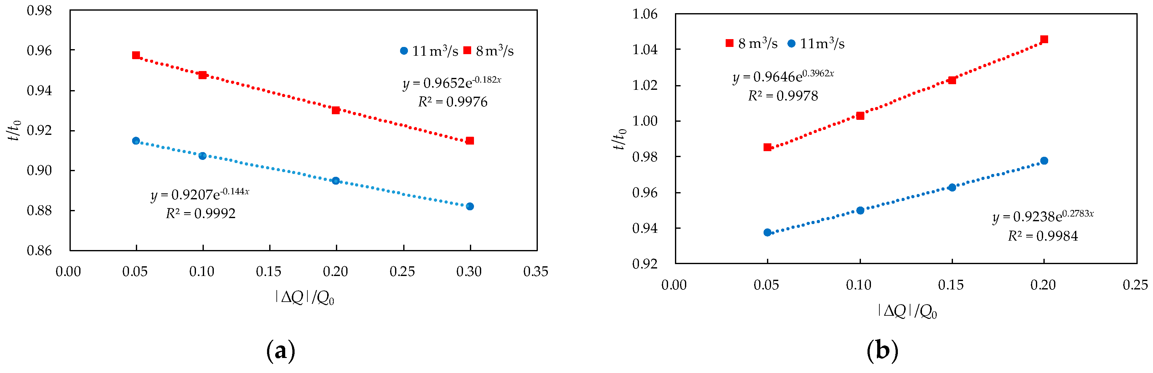
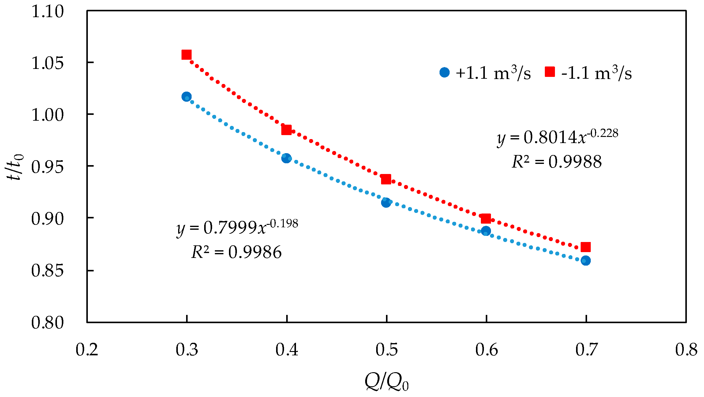
4.3.2. Effects of Variable Discharge

Eight variable discharges (−20%, −15%, −10%, −5%, +5%, +10%, +20%, and +30% of the design discharge) and one water level immediately upstream of the pumping station (4.04 m, 80% of the design water depth) were set according to the design discharge of G1–P1. The control time of P1 (t) was calculated using initial discharges of 8.8 m³/s (40% of the design discharge) and 11 m³/s (50% of the design discharge). The design discharge was taken as the base discharge (Q₀) and the time obtained by dividing the channel length by the design flow velocity was taken as the base time (t₀). The calculation results are dimensionless and are shown in Figure 8.

Figure 8a shows that t/t₀ decreased with the increase of |∆Q|/Q₀ when the discharge increased, indicating that increasing the discharge could reduce the control time, and the larger the increase of the discharge, the shorter the control time. Figure 8b shows that t/t₀ increased with the increase of |∆Q|/Q₀ when the discharge decreased, indicating that decreasing the discharge could increase the control time, and the larger the decrease of discharge, the longer the control time. There was an exponential relationship between |∆Q|/Q₀ and t/t₀.

Table 2 shows that the propagation velocity increased with the increase of the discharge. Given that the initial discharge and water level immediately upstream of the pumping station were constant, the higher the increase of discharge in the same time, the faster the average propagation velocity, and consequently, the shorter the control time. This is consistent with the findings of Li et al. [44] in the Shitouhe irrigation area. Because the channel is trapezoidal, the propagation velocity varied nonlinearly with the discharge. It is seen from Table 2 that there was an exponential relationship between the variable discharge and the reciprocal of the propagation velocity (1/v = 0.207 × e^−0.09ΔQ, R² = 0.9989), and thus, there was an exponential relationship between |∆Q|/Q₀ and t/t₀. When the discharge increased, increasing the variable discharge could decrease the increase of the propagation velocity, while the opposite was obtained as the discharge decreased.

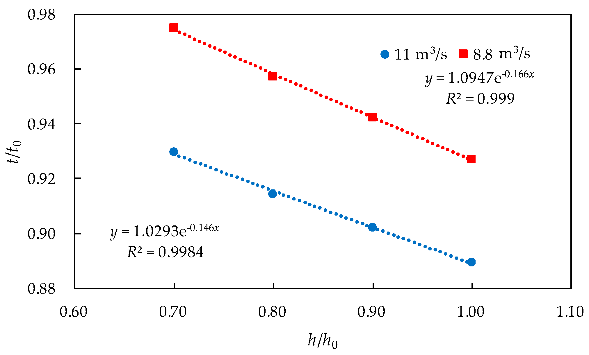
4.3.3. Effects of the Water Depth Immediately Upstream of the Pumping Station

Four water depths (70%, 80%, 90%, and 100% of the design water depth, namely, 1.69 m, 1.94 m, 2.18 m, and 2.42 m) and two initial discharges (40% and 50% of the design discharge, namely, 8.8 m³/s and 11 m³/s) were set according to the actual situation of G1–P1. The control time of P1 (t) was calculated when the discharge at G1 was increased by 1.1 m³/s. The design water depth was taken as the base water depth (h₀), and the time obtained by dividing the channel length by the design flow velocity was taken as the base time (t₀). The calculation results are dimensionless and are shown in Figure 9.

Figure 9 shows that as the upstream discharge was increased by 1.1 m³/s at an initial discharge of 11.0 m³/s, t/t₀ reached a maximum at a water depth of 1.69 m (h/h₀ = 0.70) and a minimum at a water depth of 2.42 m (h/h₀ = 1.00). The higher the water depth, the shorter the control time, and there was an exponential relationship between the control time and the water depth. Similar results were obtained at an initial discharge of 8.8 m³/s. Thus, the control time decreased with the increase of water depth immediately upstream of the pumping station.

The flow and wave velocities at different water depths were calculated. Given constant initial and variable discharges, the water depth immediately upstream of the pumping station increased the water depth of the downstream channel but had no effect on the upstream channel, resulting in an increase in wave velocity but a decrease in flow velocity. As the increase of the wave velocity was greater than the decrease of flow velocity in the channel, the propagation velocity of the flow increased gradually, resulting in a decrease in the control time. Because the wave velocity is proportional to the square root of water depth, the increase in wave velocity decreased with the increase of water depth. It can be seen from

Table 3. Hydraulic parameters under different water depths.

Water Depth Upstream of P1 (m)	Channel Section		Water Depth (m)	Wetted Cross-Sectional Area (m2)	Flow Velocity (m/s)	Wave Velocity (m/s)	Propagation Velocity (m/s)
1.69	Downstream of G1	Before change	1.98	17.69	0.62	4.40	5.02
		After change	2.09	19.19	0.63	4.53	5.16
	Upstream of S1	Before change	2.32	22.42	0.49	4.77	5.26
		After change	2.44	24.11	0.50	4.89	5.39
	Downstream of U1	Before change	1.56	12.70	0.87	3.92	4.79
		After change	1.59	13.04	0.93	3.95	4.88
	Upstream of P1	Before change	1.69	14.16	0.78	4.07	4.85
		After change	1.69	14.16	0.85	4.07	4.93
1.94	Downstream of G1	Before change	1.98	17.68	0.62	4.40	5.02
		After change	2.09	19.18	0.63	4.53	5.16
	Upstream of S1	Before change	2.32	22.40	0.49	4.77	5.26
		After change	2.44	24.09	0.50	4.89	5.39
	Downstream of U1	Before change	1.75	14.82	0.74	4.14	4.88
		After change	1.76	15.06	0.80	4.16	4.96
	Upstream of P1	Before change	1.94	17.23	0.64	3.36	5.00
		After change	1.94	17.23	0.70	4.36	5.06
2.18	Downstream of G1	Before change	1.97	17.66	0.62	4.40	5.02
		After change	2.09	19.16	0.63	4.53	5.16
	Upstream of S1	Before change	2.32	22.37	0.49	4.77	5.26
		After change	2.44	24.06	0.50	4.89	5.39
	Downstream of U1	Before change	1.95	17.31	0.63	4.37	5.00
		After change	1.96	17.48	0.69	4.38	5.07
	Upstream of P1	Before change	2.18	20.40	0.54	4.62	5.16
		After change	2.18	20.40	0.59	4.62	5.21
2.42	Downstream of G1	Before change	1.97	17.61	0.62	4.40	5.02
		After change	2.08	19.11	0.63	4.52	5.15
	Upstream of S1	Before change	2.32	22.31	0.49	4.77	5.26
		After change	2.43	24.01	0.50	4.89	5.39
	Downstream of U1	Before change	2.16	20.18	0.54	4.61	5.15
		After change	2.17	20.30	0.60	4.62	5.22
	Upstream of P1	Before change	2.42	23.81	0.46	4.87	5.33
		After change	2.42	23.81	0.51	4.87	5.38

that the decrease in the reciprocal wetted cross-sectional area decreased with the increase of water depth, and thus, the decrease of the flow velocity decreased with the increase of the water depth. Because the variation in flow velocity decrease was greater than that of the wave velocity increase, the increase in the propagation velocity and the decrease in the control time increased with the increase of the water depth. It is seen from Table 3 that there was an exponential relationship between water depth and the reciprocal of the average propagation velocity (1/v = 0.2184 × e^−0.056h, R² = 0.9941), and thus, there was an exponential relationship between h/h₀ and t/t₀.

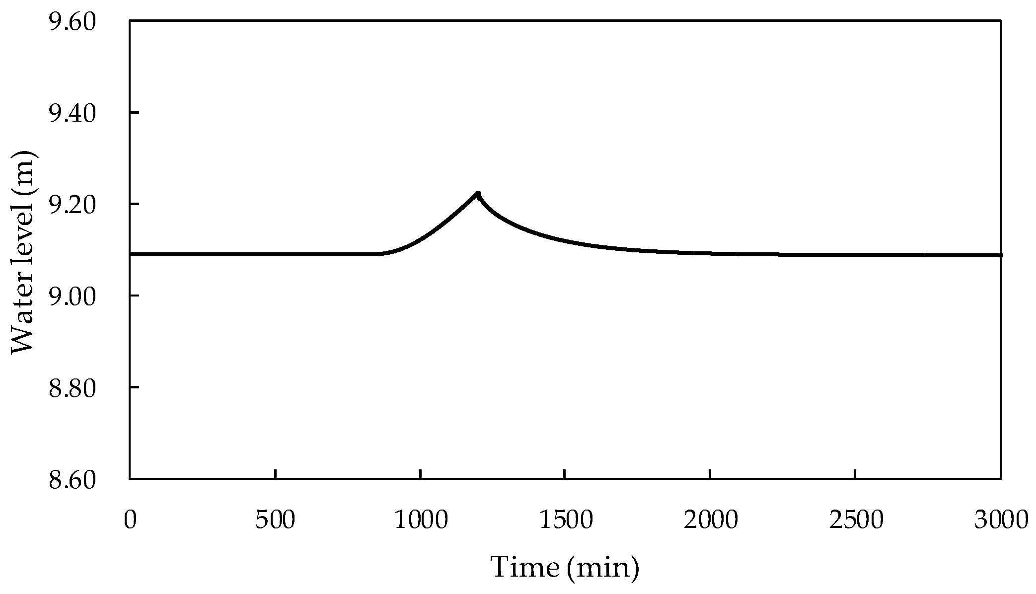
4.4. Joint Control of the Cascade Pumping Stations

The joint control of the cascade pumping stations from the Songzhuang sluice gate (G1) to the Dongsong pumping station (P2) was analyzed as an example. The initial discharge was 11 m³/s, the water level immediately upstream of P1 and P2 were 4.04 m and 9.09 m, respectively, and the variable discharge was 1.1 m³/s. The control time of P1 was 728 min and the control time of P2 was 1204 min. The variation of the water level immediately upstream of P1 and P2 are shown in Figure 6b and Figure 10, respectively. The water levels immediately upstream of P1 and P2 returned to the original water level after a short period of fluctuation, with variations of only 14 cm and 12 cm, respectively, which can ensure the safe operation of the pumping station.

The initial discharge was 11 m³/s, the water levels immediately upstream of P1 and P2 were 4.04 m and 9.09 m, and the variable discharge was 4.4 m³/s. The control time of P1 was 712 min and that of P2 was 1198 min. The variations of the water level immediately upstream of P1 and P2 are shown in Figure 11. Due to the small water storage capacity of G1–P2, the water levels immediately upstream of P1 and P2 changed dramatically by 48 cm and 53 cm, respectively. Generally, the variation of the water level in an open channel should not exceed 30 cm per day. Thus, the proposed method is more applicable to water diversion projections with wide channels and a high storage capacity, and a multi-step control method should be considered for narrow channels with dramatic changes in the discharge.

5. Conclusions

A simple method was proposed in this study to determine the control time of a pumping station to ensure the stability of the water level immediately upstream of the pumping station in an open channel. A case study was performed using G1–P1 of the Jiaodong water diversion project, where the effects of the initial discharge, variable discharge, and water level on the control time were investigated. The main conclusions are as follows: (1) The greater the initial discharge, the greater the flow velocity and wave velocity, and consequently, the smaller the control time. There was a power function relationship between the initial discharge and the control time of the pumping station. (2) Increasing the upstream discharge reduced the control time, while decreasing the upstream discharge increased the control time. (3) The control time decreased with the increase of the water depth immediately upstream of the pumping station.

However, some limitations of the proposed method should also be noted. The upstream variable discharge should be kept consistent with the discharge of pumping units. In addition, this method is more applicable to water diversion projects with wide channels and a large storage capacity. Dramatic changes may occur in the water level immediately upstream of the pumping station when the upstream discharge changes significantly or the channel is narrow. In this case, the critical water level is likely to be exceeded, and thus, a multi-step control method should be considered in future research. In this study, the characteristic curve of the pumping station was not considered, which should be considered in future research.

References

1. Zhang, C.; Li, M.; Guo, P. An interval multistage joint-probabilistic chance-constrained programming model with left-hand-side randomness for crop area planning under uncertainty. J. Clean. Prod. 2017, 167, 1276–1289. [Google Scholar] [CrossRef]
2. Wang, Y.; Li, Z.; Guo, S.; Zhang, F.; Guo, P. A risk-based fuzzy boundary interval two-stage stochastic water resources management programming approach under uncertainty. J. Hydrol. 2020, 582, 124553. [Google Scholar] [CrossRef]
3. Kerim, E.D.; David, A.D. Drivers of interbasin transfers in the United States: Insights from sampling. J. Am. Water Resour. Assoc. 2019, 55, 1038–1052. [Google Scholar]
4. Wang, L.; Yan, D.; Wang, H.; Yin, J.; Bai, Y. Impact of the Yalong-Yellow River water transfer project on the eco-environment in Yalong River basin. Sci. China Technol. Sci. 2013, 56, 831–842. [Google Scholar] [CrossRef]
5. Xi, S.; Wang, B.; Liang, G.; Li, X.; Lou, L. Inter-basin water transfer-supply model and risk analysis with consideration of rainfall forecast information. Sci. China Technol. Sci. 2010, 53, 3316–3323. [Google Scholar] [CrossRef]
6. Lu, L.; Tian, Y.; Lei, X.; Wang, H.; Qin, T.; Zhang, Z. Numerical analysis of the hydraulic transient process of the water delivery system of cascade pump stations. Water Sci. Technol. Water Suppl. 2018, 18, 1635–1649. [Google Scholar] [CrossRef]
7. Abdallah, M.; Kapelan, Z. Iterative extended lexicographic goal programming method for fast and optimal pump scheduling in water distribution networks. J. Water Resour. Plan. Manag. 2017, 143, 04017066. [Google Scholar] [CrossRef]
8. Bagirov, A.M.; Barton, A.F.; Mala-Jetmarova, H.; Al Nuaimat, A.; Ahmed, S.; Sultanova, N.; Yearwood, J. An algorithm for minimization of pumping costs in water distribution systems using a novel approach to pump scheduling. Math. Comput. Model. 2013, 57, 873–886. [Google Scholar] [CrossRef]
9. Wu, P.; Lai, Z.N.; Wu, D.Z.; Wang, L. Optimization research of parallel pump system for improving energy efficiency. J. Water Resour. Plan. Manag. 2015, 141, 04014094. [Google Scholar] [CrossRef]
10. Georgescu, S.C.; Georgescu, A.M. Application of HBMOA to pumping stations scheduling for a water distribution network with multiple tanks. Procedia Eng. 2014, 70, 715–723. [Google Scholar] [CrossRef] [Green Version]
11. Iglesias-Rey, P.L.; Martínez-Solano, F.J.; Mora Meliá, D. Combining Engineering judgment and an optimization model to increase hydraulic and energy efficiency in water distribution networks. J. Water Resour. Plan. Manag. 2015, 142, C4015012. [Google Scholar] [CrossRef]
12. Zhang, Z.; Lei, X.; Tian, Y.; Wang, L.; Wang, H.; Su, K. Optimized scheduling of cascade pumping stations in open-channel water transfer systems based on station skipping. J. Water Resour. Plan. Manag. 2019, 145, 05019011. [Google Scholar] [CrossRef]
13. Boxall, J.B.; Mounce, S.R.; Ostojin, S. An artificial intelligence approach for optimizing pumping in sewer systems. J. Hydroinform. 2011, 13, 295–306. [Google Scholar]
14. Nowak, D.; Krieg, H.; Bortz, M.; Geil, C.; Knapp, A.; Roclawski, H.; Böhle, M. Decision support for the design and operation of variable speed pumps in water supply systems. Water 2018, 10, 734. [Google Scholar] [CrossRef] [Green Version]
15. Price, E.; Ostfeld, A. Optimal pump scheduling in water distribution systems using graph theory under hydraulic and chlorine constraints. J. Water Resour. Plan. Manag. 2016, 142, 04016037. [Google Scholar] [CrossRef]
16. Petrollese, M.; Seche, P.; Cocco, D. Analysis and optimization of solar-pumped hydro storage systems integrated in water supply networks. Energy 2019, 189, 116176. [Google Scholar] [CrossRef]
17. Sang, G.; Cao, S.; Guo, R.; Zhang, L. Optimization of cost per day of cascade pumping station water-delivery system. J. Drain. Irrig. Mach. Eng. 2013, 31, 688–695. [Google Scholar]
18. Zheng, H.; Zhang, Z.; Wu, H.; Lei, X. Study on the daily optimized dis-patching and economic operation of cascade pumping stations in water conveyance system. J. Hydraul. Eng. 2016, 47, 1558–1565. [Google Scholar]
19. Liu, X.; Tian, Y.; Lei, X.; Wang, H.; Liu, Z.; Wang, J. An improved self-adaptive grey wolf optimizer for the daily optimal operation of cascade pumping stations. Appl. Soft Comput. 2019, 75, 473–493. [Google Scholar] [CrossRef]
20. Zhuan, X.; Zhang, L.; Li, W.; Yang, F. Efficient operation of the fourth huaian pumping station in east route of south-to-north water diversion project. Int. J. Electr. Power Energy Syst. 2018, 98, 399–408. [Google Scholar] [CrossRef]
21. Gong, Y.; Cheng, J. Optimization of cascade pumping stations’ operations based on head decomposition–dynamic programming aggregation method considering water level requirements. J. Water Resour. Plan. Manag. 2018, 144, 04018034. [Google Scholar] [CrossRef]
22. Malaterre, P.O.; Rogers, D.C.; Schuurmans, J. Classification of canal control algorithms. J. Irrig. Drain. Eng. 1998, 124, 3–10. [Google Scholar] [CrossRef] [Green Version]
23. Bautista, E.; Clemmens, A.J. Volume compensation method for routing irrigation canal demand changes. J. Irrig. Drain. Eng. 2005, 131, 494–503. [Google Scholar] [CrossRef] [Green Version]
24. Isapoor, S.; Montazar, A.; Van Overloop, P.J.; Van De Giesen, N. Designing and evaluating control systems of the Dez main canal. Irrig. Drain. 2011, 60, 70–79. [Google Scholar] [CrossRef]
25. Malaterre P, O. Pilote: Linear quadratic optimal controller for irrigation canals. J. Irrig. Drain. Eng. 1998, 124, 187–194. [Google Scholar] [CrossRef]
26. Tian, X.; van Overloop, P.; Negenborn, R.R.; Van De Giesen, N. Operational flood control of a low-lying delta system using large time step Model Predictive Control. Adv. Water Resour. 2015, 75, 1–13. [Google Scholar] [CrossRef]
27. Wahlin, B.T.; Clemmens, A.J. Automatic downstream water-level feedback control of branching canal networks: Simulation results. J. Irrig. Drain. Eng. 2006, 132, 208–219. [Google Scholar] [CrossRef] [Green Version]
28. Kong, L.; Lei, X.; Wang, H.; Long, Y.; Lu, L.; Yang, Q. A model predictive water-level difference control method for automatic control of irrigation canals. Water 2019, 11, 762. [Google Scholar] [CrossRef] [Green Version]
29. García, L.; Barreiro-Gomez, J.; Escobar, E.; Téllez, D.; Quijano, N.; Ocampo-Martinez, C. Modeling and real-time control of urban drainage systems A review. Adv. Water Resour. 2015, 85, 120–132. [Google Scholar] [CrossRef] [Green Version]
30. Chang, F.J.; Chang, K.Y.; Chang, L.C. Counterpropagation fuzzy-neural network for city flood control system. J. Hydrol. 2008, 358, 24–34. [Google Scholar] [CrossRef]
31. Hsu, N.-S.; Huang, C.-L.; Wei, C.-C. Intelligent real-time operation of a pumping station for an urban drainage system. J. Hydrol. 2013, 489, 85–97. [Google Scholar] [CrossRef]
32. Mullapudi, A.; Lewis, M.J.; Gruden, C.L.; Kerkez, B. Deep reinforcement learning for the real time control of stormwater systems. Adv. Water Res. 2020, 140, 103600. [Google Scholar] [CrossRef]
33. Pereira, A.; Pinho, J.L.S.; Faria, R.; Vieira, J.M.P.; Costa, C. Improving operational management of wastewater systems. A case study. Water Sci. Technol. 2019, 80, 173–183. [Google Scholar] [CrossRef] [PubMed]
34. Eker, I.; Kara, T. Operation and control of a water supply system. ISA Trans. 2003, 42, 1–13. [Google Scholar] [CrossRef]
35. Abdulrahman, A.; Nasher, N. Water supply network system control based on model predictive control. J. King Saud Univ.—Eng. Sci. 2010, 22, 119–126. [Google Scholar] [CrossRef]
36. Wu, Z.; Luo, H.; Liu, C.; Sun, L.; Zhao, P. Start-up time difference of pumping station of Nansi Lake in the South-to-North water transfer. South North Water Transf. Water Sci. Technol. 2008, 6, 77–80, 91. [Google Scholar]
37. Gao, X.; Nie, X.; Sun, B.; Zhang, C. Study on opening time difference of the adjacent multi-stages pump stations in water transfer projects. J. Hydraul. Eng. 2016, 47, 1502–1509. [Google Scholar]
38. Shang, Y.; Liu, R.; Li, T.; Zhang, C.; Wang, G. Transient flow control for an artificial open channel based on finite difference method. Sci. China Technol. Sci. 2011, 54, 781–792. [Google Scholar] [CrossRef]
39. Lu, L.; Lei, X.; Tian, Y.; Wu, H. Research on the characteristic of hydraulic response in open channel of the cascade pumping station project in an emergent state. J. Basic Sci. Eng. 2018, 26, 263–275. [Google Scholar]
40. Goodwin, P.; Lyn, D.A. Stability of a general preissmann scheme. J. Hydraul. Eng. 1987, 113, 16–28. [Google Scholar]
41. Wang, C.; Yang, J.; Nilsson, H. Simulation of water level fluctuations in a hydraulic system using a coupled liquid-gas model. Water 2015, 7, 4446–4476. [Google Scholar] [CrossRef] [Green Version]
42. Hu, J.; Yang, S.; Fu, X. Experimental investigation on propagating characteristics of sinusoidal unsteady flow in open-channel with smooth bed. Sci. China Technol. Sci. 2012, 55, 2028–2038. [Google Scholar] [CrossRef]
43. Fan, J.; Wang, C.; Guan, G.; Cui, W. Study on the hydraulic reaction of unsteady flows in open channel. Adv. Water Sci. 2006, 17, 55–60. [Google Scholar]
44. Li, K.; Shen, B.; Li, Z.; Hao, G. Open channel hydraulic response characteristics in irrigation area based on unsteady flow simulation analysis. Trans. Chin. Soc. Agric. Eng. 2015, 31, 107–114. [Google Scholar]
Figure 1. The variation of the discharge immediately upstream of the pumping station.
Water 13 00355 g001
Figure 2. The experimental verification setup.
Water 13 00355 g002
Figure 3. The variation of the discharge of the pumping station (a) and water level immediately upstream of the pumping station (b).
Water 13 00355 g003
Figure 4. The layout of the engineering project.
Water 13 00355 g004
Figure 5. Water level simulation results at the S5 (a) and S6 (b) inlets.
Water 13 00355 g005
Figure 6. The variation of the discharge of the pumping station (a) and water level immediately upstream of the pumping station (b).
Water 13 00355 g006
Figure 7. Relationship between Q/Q0 and t/t0.
Water 13 00355 g007
Figure 8. Relationship between |∆Q|/Q0 and t/t0 for increasing (a) and decreasing discharge (b).
Water 13 00355 g008
Figure 9. Relationship between h/h0 and t/t0 when the upstream discharge was increased by 1.1 m3/s.
Water 13 00355 g009
Figure 10. Variation of the water level immediately upstream of P2 when the upstream discharge was increased by 1.1 m3/s.
Water 13 00355 g010
Figure 11. Variation of the water levels immediately upstream of P1 (a) and P2 (b) when the upstream discharge was increased by 4.4 m3/s.
Water 13 00355 g011