Evaluation of Improved Model to Accurately Monitor Soil Water Content

Abstract

The accurate monitoring of soil water content during the growth of crops is of great importance to improve agricultural water use efficiency. The Campbell model is one of the most widely used models for monitoring soil moisture content from soil thermal conductivities in farmland, which always needs to be calibrated due to the lack of adequate original data and the limitation of measurement methods. To precisely predict the water content of complex soils using the Campbell model, this model was evaluated by investigating several factors, including soil texture, bulk density and organic matter. The comparison of the R² and the reduced Chi-Sqr values, which were calculated by Origin, was conducted to calibrate the Campbell model calculated. In addition, combining factors of parameters, a new parameter named m related to soil texture and the organic matter was firstly introduced and the original fitting parameter, E, was improved to an expression related to clay fraction and the organic matter content in the improved model. The soil data collected from both the laboratory and the previous literature were used to assess the revised model. The results show that most of the R² values of the improved model are >0.95, and the reduced Chi-Sqr values are <0.01, which presents a better matching performance compared to the original. It is concluded that the improved model provides more accurate monitoring of soil water content for water irrigation management.

1. Introduction

Currently, more than 70% of agricultural water resources around the world are occupied by field crop irrigation [1,2], while the global average irrigation efficiency is only 50% [3,4,5]. Especially in China, the irrigation water use efficiency is only 30~40% [6,7], which is even lower than the worldwide level. The main factor of low irrigation efficiency is that the soil water content of farmland cannot be accurately monitored, which leads to irrationality in the formulation of the irrigation system, and it is impossible to accurately irrigate, resulting in wasted water resources over time. Wealth production and industrial growth are inseparable from the efficient use of water resources in agriculture [8,9], and it is important to accurately monitor soil water in real time, which helps to formulate a reasonable irrigation plan for realizing automated irrigation, increasing the irrigation water utilization coefficient, and optimizing the reasonable distribution of water resources [10,11,12,13,14].

Several methods of monitoring soil water content have been researched, such as time domain reflectometry, gravimetric sampling [15,16], the remote sensing measurement, the neutron detector method, and so on [17]. Among them, the prediction of soil moisture content from soil thermal properties has attracted the attention of many scholars [18,19,20,21,22]. The relationship between thermal characteristics and soil moisture can not only accurately estimate the soil moisture content, but also be helpful to explore the laws of soil water movement. The most widely used empirical model to determine soil water content based on thermal conductivity was presented by Campbell [20], which was applied in many later studies and instrument developments [23,24,25].

However, due to the complexity of field crops and soil conditions, as well as the differences in soil properties in each region, the estimated results of the Campbell model have been proven to have large errors in many cases [26,27]. The internal factors refer to the properties of the soil itself (such as its texture and composition [28]). Additionally, the external factors are those that can be controlled artificially, such as the porosity and organic matter content [29,30].

Researchers have analyzed and explored the Campbell model in multiple directions, and found that it is greatly affected by soil texture, compaction, and organic matter content, and large errors have occurred in estimating the water content of various types of soil [31,32]. Mahdavi et al. found the Campbell model was affected by the degree of compaction and the particle shape [33]. Wallen et al. explored the influence of soil texture on the Campbell model and proposed that the model needs to be improved [34]. Zhao et al. found that the Campbell model has large errors in the estimation of soil moisture content and thermal conductivity under high organic matter content and high temperature [35].

Some researchers have tried to calibrate the data estimated by the Campbell model for specific soil [11,34,36], but no improvement plan was proposed for the Campbell model to expand the applicable soil range. Therefore, focusing on the influencing factors of the Campbell model and improving its coefficients to accurately monitor water content of different soils will be of great importance to improve the efficiency of soil moisture monitoring. To improve the accuracy of soil water content evaluated from soil thermal conductivities by the Campbell model, this study investigated several influencing factors to assess the error of the λ~θ curve simulated by the Campbell model. In addition, the coefficients of the Campbell model were revised to reduce the error and the improved model was evaluated by the soil data from both laboratory and previous studies.

2. Materials and Methods

2.1. Soil Description

Ten soil samples with different geological conditions taken from various farmlands across five provinces of China including Jiangsu, Shandong, Hunan, Yunnan and Sichuan were measured in this study in the State Key Lab of Hydrology—Water Resources and Hydraulic Engineering, Hohai University, China. The particle size of soil distribution was determined by the pipette method [37] and classified according to the USDA standards, and the bulk density was determined by the cutting ring method [38]. The organic matter content was measured by the Automated Dry Combustion (ADC) method [39] and the total salt content of the soil was determined by the mass method [40]. These 10 soil samples are used to construct different test groups and verify the final modified model.

Table 1. Physical properties of 10 soil samples from different areas in China.

Sample Code	Type of Soil	Texture			Organic Matter	Salinity	Bulk Density
		Sand	Silt	Clay
		%					g cm−3
Soil 1	Sand	90	8	2	0.04	0.031	1.35
Soil 2	Loamy sand	78	21	1	0.89	0.041	1.36
Soil 3	Loamy sand	79	14	7	0.16	0.122	1.49
Soil 4	Loamy sand	76	13	11	0.01	0.083	1.45
Soil 5	Loam	20	70	10	0.53	0.010	1.42
Soil 6	Sandy loam	62	21	17	0.22	0.053	1.37
Soil 7	Loam	49	31	20	1.25	0.008	1.47
Soil 8	Silt loam	12	65	23	3.50	0.026	1.56
Soil 9	Clay loam	52	15	33	1.60	0.244	1.54
Soil 10	Clay	25	15	60	0.92	0.015	1.49

lists the raw soil characteristics.

2.2. Experiment Design

2.2.1. Sample Preparation for Evaluating the Campbell Model

To research the influencing factors of the Campbell model, the experiments were divided into three parts, each of which corresponds to one factor. This study adopted the controlled variable method and soils from Table 1 were chosen to be prepared into proper samples for research purposes. All prepared soil samples were placed in a cylindrical aluminum box (30 mm of height and 50 mm of diameter), and each prepared soil sample had five parallel samples. Each soil sample was tested three times and the average value was taken.

When studying the influence of soil texture, the selection and process of soils 1, 4, 5, 6, and 10 were according to the largest bulk density, organic matter, and salt content, which ensured that other factors, except soil composition, were in the same condition. Soil samples were air-dried and sieved before being filled into an aluminum box. According to the organic matter content of 0.92% and the salt content of 0.083%, peat moss and NaCl were mixed into the sample. When the bulk density was less than the set 1.55 g cm⁻¹, the triaxial compression was used to ensure that the physical properties of the soil sample other than the particle composition are maintained.

When exploring the influence of bulk density, soil 1 was chosen due to its small initial bulk density, which can be compressed to prepare soil samples with larger bulk densities. Soil 1 was air-dried and sieved before being placed in the aluminum boxes. Since the volume of the aluminum box was fixed, it was necessary to weigh different qualities of Soil 1 and compress them into aluminum boxes with the triaxial compression instrument [41].

When researching the influence of the organic matter, considering the interaction of clay content on soil organic matter [42], and when studying organic matter content as the influencing factor, soils with different textures were studied separately. Soils 1 and 10 were chosen to be prepared and peat moss was used as additional organic matter to provide different organic matter fraction samples [43]. After the soil was air-dried and sieved, peat moss was mixed into the soil sample according to five set organic content levels of 0.04%, 0.2%, 0.8%, 1.6%, and 3.0% [36,44]. After that, the bulk density was re-measured and adjusted to ensure that every sample was in the same bulk density state.

Table 2. Soil samples for evaluating the factors influencing the Campbell model.

Influencing Factors	Sample Code	Type of Soil	Texture			Organic Matter	Salinity	Bulk Density
			Sand	Silt	Clay
			%					g cm−3
Texture	S	Sand	90	8	2	0.92	0.09	1.55
	LS	Loamy sand	76	13	11
	SLL	Silt Loam	20	70	10
	SDL	Sandy loam	62	21	17
	C	Clay	25	15	60
Bulk density	BD1.35	Sand	90	8	2	0.04	0.031	1.35
	BD1.45							1.45
	BD1.50							1.50
	BD1.55							1.55
	BD1.60							1.60
Organic matter	SOM0.04	Sand	90	8	2	0.04	0.031	1.45
	SOM0.2					0.2
	SOM0.8					0.8
	SOM1.6					1.6
	SOM3.0					3.0
	COM0.04	Clay	25	15	60	0.04	0.015	1.49
	COM0.2					0.2
	COM0.8					0.8
	COM1.6					1.6
	COM3.0					3.0

lists the basic properties of soil samples to explore the influencing factors of the λ~θ model.

2.2.2. Calibration of the Revised Model

Soils listed in Table 1 were prepared to calibrate the revised model. After being dried and sieved, each kind of soil was weighed into five equal parts and placed in aluminum boxes according to a consistent operation process, that is, there were five parallel samples of each kind of soil. Water with different quality was added and mixed. Measurements were conducted from five different locations of each sample to average the error of measurement of thermal conductivities. The relationship curve between soil thermal conductivity and water content was drawn and compared with the improved model.

2.2.3. Soil Thermal Properties and Water Content Measurement

The thermal conductivities of the soil throughout the entire experiment were measured using a KD2 Pro. The thermal conductivity detector KD2 Pro developed by Decagon has been proven to be relatively highly accurate by many researchers [45,46]. Additionally, the data measured by the KD2 Pro were used to represent the actual thermal conductivities [47].

To show the influence of these factors on the model curve more intuitively, the method of actively adding water was adopted to obtain a quantitative soil water value, so that the disturbance of organic matter and salinity during each drying process could be avoided. For each set of experiments, the same quality of water was mixed into each aluminum box at the same time. All the samples were sealed with plastic wrap for 24 h. During the water injection process, the soil was completely filled in the aluminum box, and each sample weighed again to avoid the overflow of solid materials due to the injection of water.

2.3. Evaluation Methods

2.3.1. The Campbell Model

In 2010, the Campbell model was used to explore the feasibility of optical fiber for distributed soil water measurement [48], which provided a theoretical basis for the real-time monitoring of soil water status, automatic irrigation, and field management [49]. Since soil thermal conductivity is an inherent property of soil and even water is constantly changing, Campbell takes soil water as the independent variable and soil thermal conductivity as the dependent variable. The model expression and the parameters are as follows:

$$\mathsf{\lambda }=\mathrm{A}+\mathrm{B}\mathsf{\theta }-\left(\mathrm{A}-\mathrm{D}\right)\exp \left[-{(\mathrm{C}\mathsf{\theta })}^{\mathrm{E}}\right]$$

(1)

The coefficient A is determined by the volume fraction of quartz and other minerals:

$$\mathrm{A}=\frac{0.57+1.73{\varphi }_q+0.93{\varphi }_m}{1-0.74{\varphi }_q-0.49{\varphi }_m}-2.8{\varphi }_s\left(1-{\varphi }_s\right)$$

(2)

where ${\varphi }_q$ is the volume fraction of quartz, ${\varphi }_m$ is the volume fraction of other minerals and ${\varphi }_s$ is the solid fraction of the soil, which equals the sum of ${\varphi }_q$ and ${\varphi }_m$. The coefficients B, C, D, and E are given as

$$\mathrm{B}=1.06{\rho }_b$$

(3)

$$\mathrm{C}=1+\frac{2.6}{{\varphi }_{clay}{}^{1/2}}$$

(4)

$$\mathrm{D}=0.03+0.1{\rho }_b{}^2$$

(5)

$$\mathrm{E}=4$$

(6)

where ${\rho }_b$ is the bulk density of the soil and ${\varphi }_{clay}$ is the clay content, and the particle density of mineral soil is assumed to be 2.65 g cm⁻³. The parameters B and D are determined by the bulk density of the soil, C is associated with the clay content, which determines the water content where the thermal conductivity starts rising rapidly, and E is the fitting parameter of the curve [20].

It can be seen that the parameters in the Campbell model, except for the parameter E, have certain physical meanings and are closely related to various influencing factors. By analyzing the error trend in the Campbell model curve under each influencing factor, the parameters that need to be improved can be preliminarily judged.

2.3.2. Error Analysis

This study uses R² and the reduced Chi-Sqr calculated by Origin to analyze the error between the Campbell model curve and the measured curve under each influencing factor. The R² represents the fit of the Campbell model curve to the measured value. The closer the R² is to 1, the better the fit. The reduced Chi-Sqr represents the error between the simulated curve and the measured curve [50]. When the reduced Chi-Sqr approaches 0, the error of the simulated value becomes smaller [51].

Since it is difficult to control the thermal conductivity of the soil at the same level, the study chose to verify the error between the simulated value and the measured value of the soil thermal conductivity under the same moisture content, and performed a linear fitting, of which the R² represents the fitting spend.

3. Results

3.1. Campbell Model Implications

In this part, the λ~θ curve of the measured soil samples with the Campbell model curve and quantitatively analyzed error was compared. The Campbell model also gives detailed anatomy in terms of parameter assignment, and corrections were made based on the factors influencing the parameters.

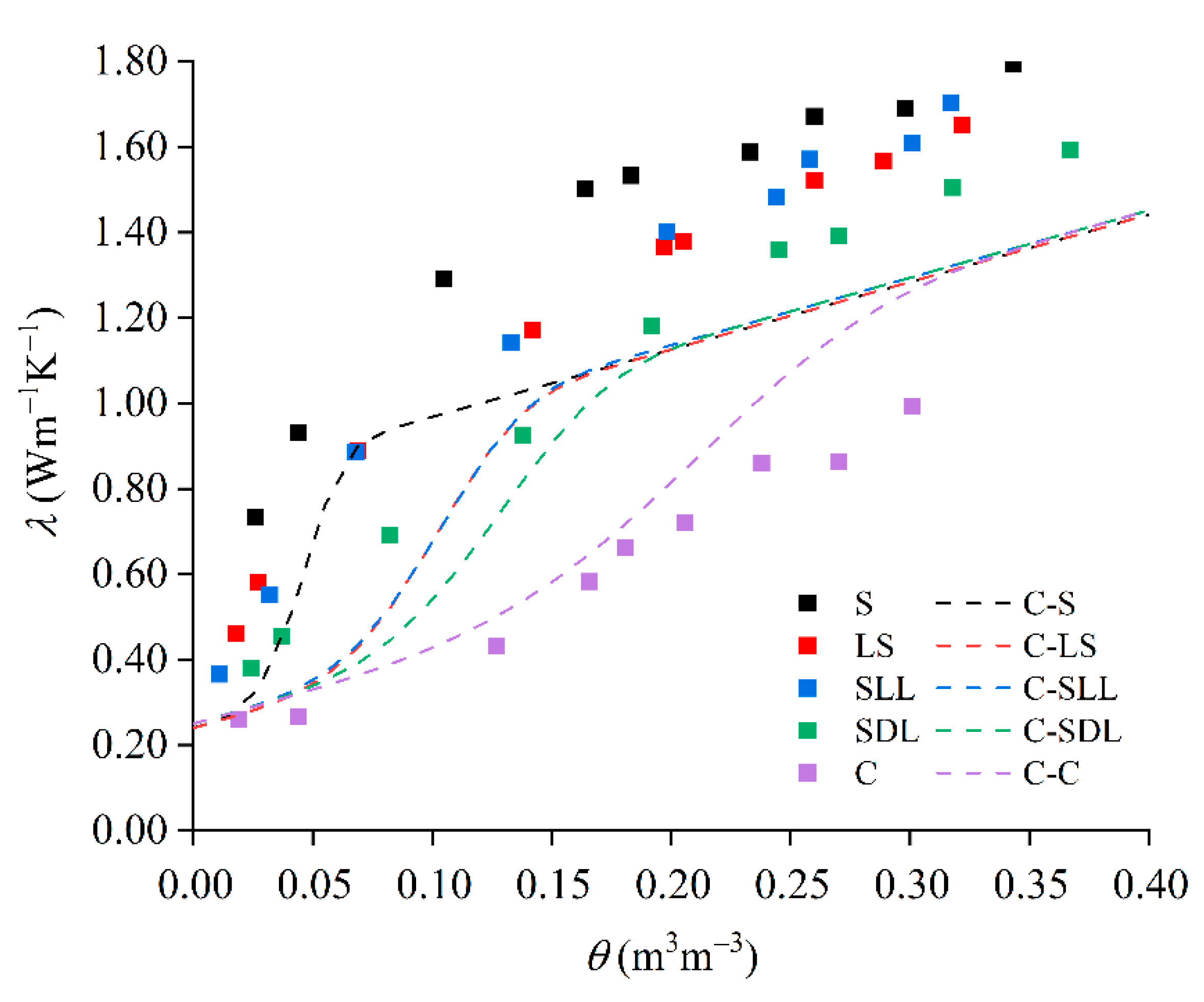
3.1.1. Among Soil with Different Textures

For soil with a specific texture, the thermal conductivity increases rapidly as the soil water content increases (Figure 1). The response shows two stages. When the water content is higher than a certain level, which is generally 0.05–0.1 m³ m⁻³, the rate gradually declines with the increase in soil thermal conductivity.

Among soils with different textures, the growth rate of thermal conductivity for sandy soil with low water content is significantly greater than that of clay soil. On a full range of water content, the thermal conductivity of coarse-grain soil for any water content is greater than that of fine-grain soil due to the high proportion of quartz [52].

The Campbell [20] model almost matched the measured data of soil sample S when the water content was <0.1 (m³ m⁻³) and that of sample C when the water content was <0.2 (m³ m⁻³). The thermal conductivities predicted by the Campbell model are always lower than the measured values, which implies that the parameters that determine the degree of increase in the model curve need to be adjusted. At full water content, R² varies in the range 0.722–0.876, with a low degree of matching and a large range. The reduced Chi-Sqr tends to decrease as the soil clay content increases (

Table 3. Reduced Chi-Sqr and R² of the measured value and the Campbell model simulation value for soils with different textures.

Soil Code	Reduced Chi-Sqr	R2
S	0.190	0.722
LS	0.097	0.781
SLL	0.104	0.777
SDL	0.028	0.783
C	0.027	0.876

). Thus, soil texture has a great impact on the λ~θ curve, and the Campbell model showed different trends under soils with different textures, which is consistent with the research conclusion of Wallen et al. [34]. It is assumed that the error of the model curve comes from the parameters of the soil texture.

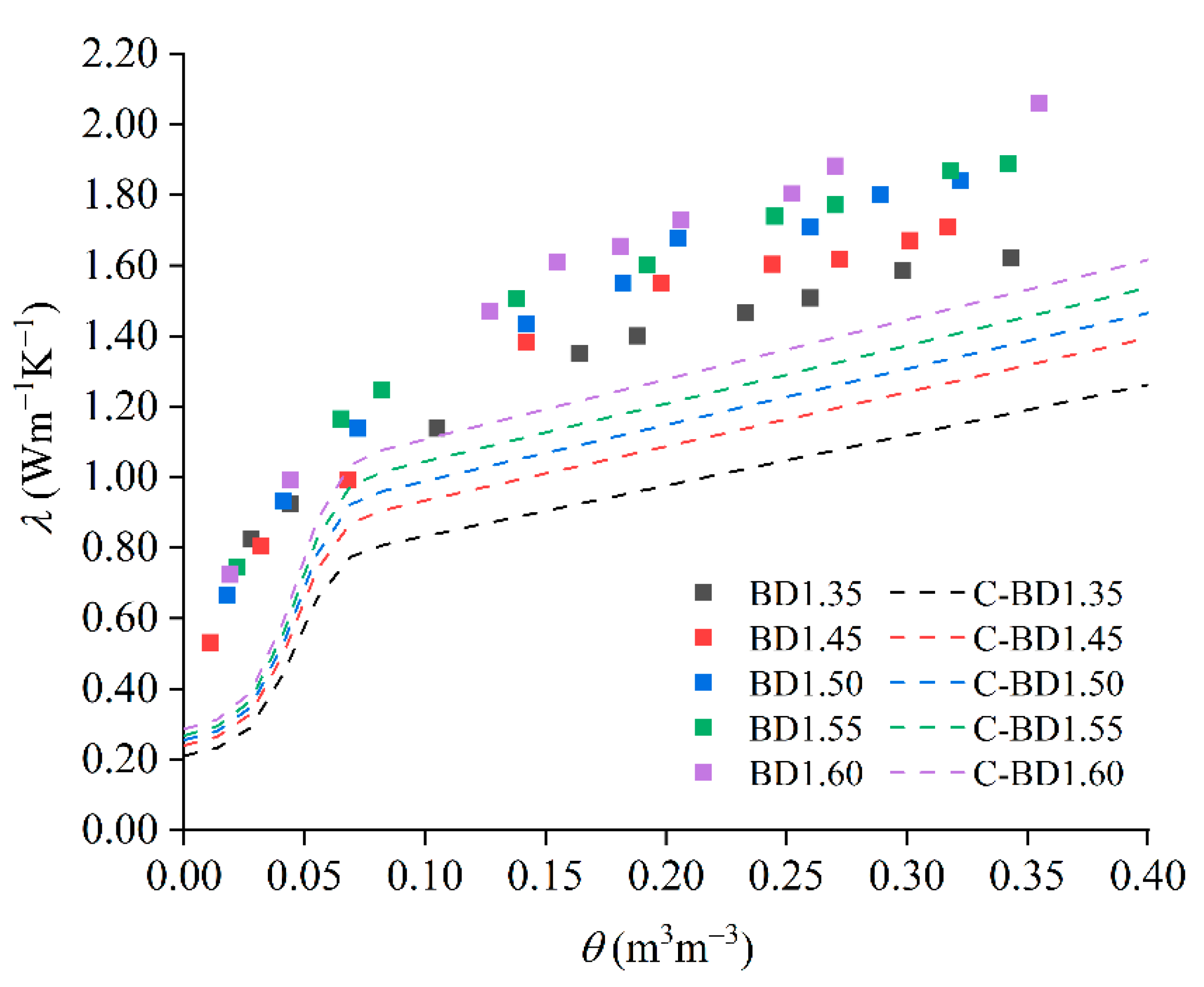
3.1.2. Among Soil with Different Bulk Densities

As is shown is Figure 2, when the water content was low (<0.05 m³ m⁻³), the difference between the λ~θ of soil samples with different bulk densities was very little. As the water content increases, the thermal conductivity of soil samples with larger bulk densities increases to a greater degree than that of soil samples with lower bulk density. The higher the dry density of the soil, the more solid matter per unit volume of the soil and the closer the soil particles are arranged. Thus, the contact area between particles increases accordingly, which ultimately leads to an increase in the soil’s thermal conductivity.

Compared with the Campbell model, R² varies in the range 0.652–0.732, which is far from 1, and the degree of matching is lower than that of the influence of soil texture (

Table 4. Reduced Chi-Sqr and R² of the measured value and the Campbell model simulation value for soils with different bulk densities.

Soil Code	Reduced Chi-Sqr	R2
BD1.35	0.219	0.652
BD1.45	0.176	0.672
BD1.50	0.210	0.655
BD1.55	0.179	0.717
BF1.60	0.201	0.732

). This may be due to the fact that particle density in the Campbell model is assumed to be 2.65 g cm⁻³, while the particle density of soils is actually in the range 2.6–2.8 g cm⁻³ [53].

Under different soil bulk density, the Campbell model curve is higher than the measured curve, that is, the influence of the soil bulk density on the Campbell model is monotonic, but because the degree of influence is less than the soil texture, it is not suitable to directly select the parameters that have a more obvious response to the curve shape for correction.

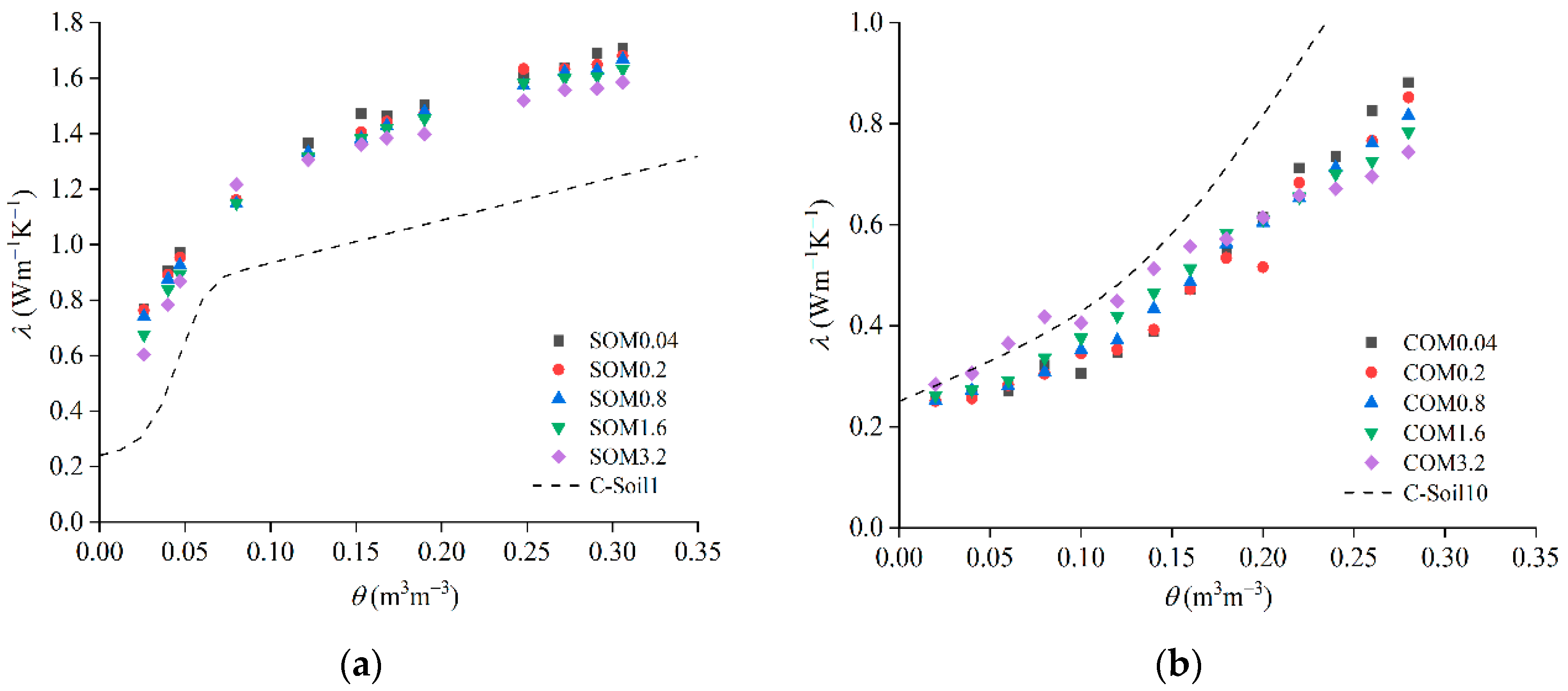
3.1.3. Among Soil with Different Organic Matter Contents

The empirical models proposed in the previous studies rarely consider the organic matter. To improve the model’s applicability and accuracy, the effects of organic matter on the model were studied with two soil texture types: sand and clay. The properties and the experimental results of samples are shown below (Figure 3).

For the sandy soil shown in Figure 3a, the soil sample with more organic matter has lower thermal conductivity for almost the entire range of water content. However, for clay soil (Figure 3b) with a low level of water content, the λ of the soil sample with more organic matter is higher than the soil containing less organic matter. Additionally, as the water content increases, the λ of the soil sample with more organic matter has a lower rate of increase and gradually becomes lower than that of samples with less organic matter.

The Campbell model does not consider the differences in soil organic matter content, that only one response model can be given for two different soil samples. In terms of the sandy soil sample, the simulation overall is small, and the R² decreases with the increase in organic matter content. For the clay soil, the model value is overall large, the deviation is greater at high water content, and the trend in R² is opposite to that of sandy soil (

Table 5. Reduced Chi-Sqr and R² of the measured value and the Campbell model simulation value for soils with different organic matter contents.

Soil Code	Reduced Chi-Sqr	R2	Soil Code	Reduced Chi-Sqr	R2
SOM0.04	0.193	0.792	COM0.04	0.037	0.748
SOM0.2	0.176	0.766	COM0.2	0.047	0.829
SOM0.8	0.161	0.744	COM0.8	0.045	0.872
SOM1.6	0.144	0.731	COM1.6	0.046	0.876
SOM3.0	0.117	0.722	COM3.0	0.050	0.892

).

The different responses of the Campbell model to organic matter on different texture soils illustrated that organic matter plays a different role for different soil textures. It can be explained that organic matter plays an important role in the water and heat coupling process [44]. Usowicz and Lipiec [29] analyzed the effect of biochar obtained from wood biomass and other organic amendments (peat and compost) on soil thermal properties and attributed the results to the addition of exogenous organic matter. In the performance of reduced Chi-Sqr and R², the λ~θ curve predicted by the Campbell model for cohesive soil was significantly better than that for sandy soil.

3.2. Summary of Error Sources in the Campbell Model Curve

• Among the various factors, Campbell has the lowest match degree of soils with different bulk densities. Therefore, it may be necessary to focus on parameters related to bulk density. The soil texture and organic matter content will affect the particle density of soil. In the Campbell model, the values of the parameters B and D default the soil particle density to 2.65 g/cm³.
• The organic matter not only reduces the density of soil particles but also interacts with clay particles in the soil, thereby affecting the parameters related to clay content in the Campbell model.
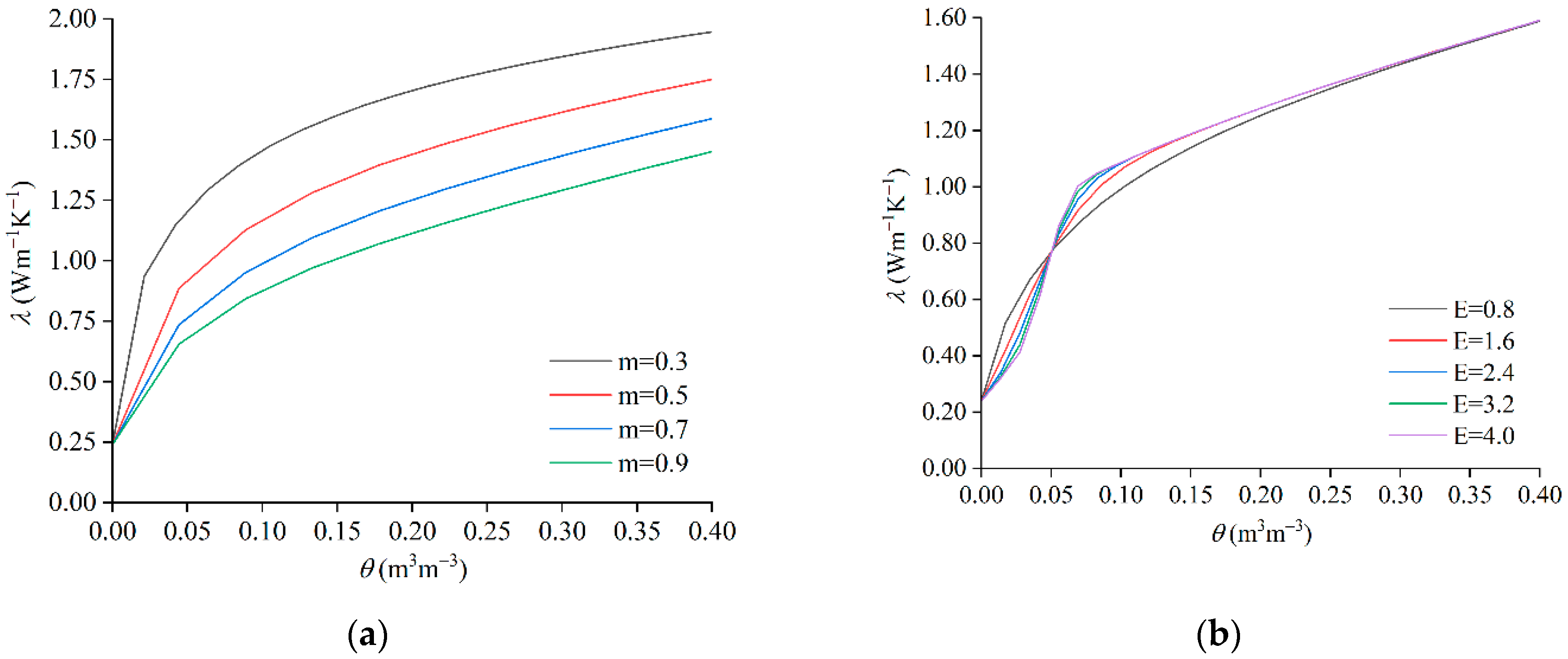
• Various parameters have different influences on the shape of the model and the parameters for correction can be determined by changes in the shape.

4. Discussion

4.1. Revised Model

The Campbell model proved through experiments that there are unequal errors under various influencing factors that need to be corrected, which is also consistent with the conclusions of other scholars. The revised empirical model attempts to improve the accuracy of the λ~θ relationship evaluation and to expand the range of water content that can match this model.

In the curve of the Campbell model, the parameters, which are C, D, and E, are in an exponential expression. Among them, the parameter E is a fitting parameter with no actual physical meaning. Therefore, the correction of the parameter E was selected rather than the parameters C and D. If the parameter E is revised, the influence of the parameters C and D on the curve could be expressed at the same time, which makes it easier to obtain a convergent solution than revising three parameters at the same time when using the least squares method to fit [54]. At the same time, the correction parameter m is introduced and the original parameter B is corrected. Since the bulk density has a smaller effect on the curve than the soil texture, and a small change in parameter B will also have a greater effect on the curve, this study chose to introduce the parameter m. The revised empirical model was proposed as follows (Equation (7)):

$$\mathsf{\lambda }=\mathrm{A}+\mathrm{B}{\mathsf{\theta }}^{\mathrm{m}}-\left(\mathrm{A}-\mathrm{D}\right)\exp \left[-{(\mathrm{C}\mathsf{\theta })}^{\mathrm{E}}\right]$$

(7)

To find the determinants of the values of parameter m and E, Soil 1 was selected as an example to analyze the influence of different m and E values in the curve (Figure 4).

Parameter m affects the degree of curve rise. As the value of m approaches 1, the curve gradually flattens, the growth rate slows, and parameter m has an influence on the thermal conductivity value under the full range of water content. As parameter E increases, the rising part of the curve steepens. Furthermore, while parameter E determines the shape of the curve when the volumetric water content is <0.3 m³ m⁻³, under high water content, changes in the value of parameter n have few effects on the curve.

It is assumed that parameter m is the matched option associated with the soil texture and organic matter and that parameter E, which replaced the parameter E proposed by Campbell, was decided by the clay fraction and organic matter. The soil sample data were used to match the measured data using the software Originlab 2021.

Table 6. The values of m and E of the soil samples.

Influencing Factors	Sample Code	m	E
Texture	S	0.468	1.211
	LS	0.619	1.362
	SLL	0.542	1.350
	SDL	0.763	1.466
	C	1.582	2.203
Bulk density	BD1.35	0.452	0.928
	BD1.45	0.454	0.931
	BD1.50	0.458	0.931
	BD1.55	0.455	0.930
	BF1.60	0.452	0.933
Organic matter	SOM0.04	0.452	0.931
	SOM0.2	0.458	0.977
	SOM0.8	0.479	1.164
	SOM1.6	0.488	1.418
	SOM3.0	0.514	1.854
	COM0.04	2.111	2.659
	COM0.2	2.119	2.595
	COM0.8	2.133	2.237
	COM1.6	2.146	1.789
	COM3.0	2.172	1.001

shows the m and E values of each soil sample.

For soil samples of different bulk densities, the values of parameter m and E are almost equal, which illustrates that the values of m and E have nothing to do with soil bulk densities. For soil samples with different textures, the values of parameter m and E tend to increase as the clay content increases. Regarding the influence of organic matter, the parameter m values of sandy soil and clay soil both increase with the increase in organic matter content. However, the changing trend for parameter E is the opposite. The parameter E of sandy soil increases in proportion with the increase in organic matter content, while that of cohesive soil decreases.

Therefore, it is assumed that the value of parameter m is related to soil texture and organic matter content, while parameter E is only related to clay content and organic matter content. We used the least-squares method to obtain the expression of the parameters m and E (Equations (8) and (9)):

$$\mathrm{m}=0.71{\phi }_{sand}+0.57{\phi }_{silt}+2.6{\phi }_{clay}+1.88{\phi }_{om}-0.28$$

(8)

$$\mathrm{E}=3.07{\phi }_{clay}+34{\phi }_{om}-151{\phi }_{clay}{\phi }_{om}+0.86$$

(9)

where ${\phi }_{sand}$ is the sand fraction, ${\phi }_{silt}$ is the silt fraction,${\phi }_{clay}$ is the clay fraction, and ${\phi }_{om}$ is the organic matter fraction.

4.2. Evaluation and Error Analysis

The model evaluation is conducted to prove the applicability of the revised model, including the range of water content. Here, two groups of data were used: the soil sample listed in Table 1 and the data from previous studies. The reduced Chi-Sqr and R² of the measured and modeled curve were used to evaluate the new model.

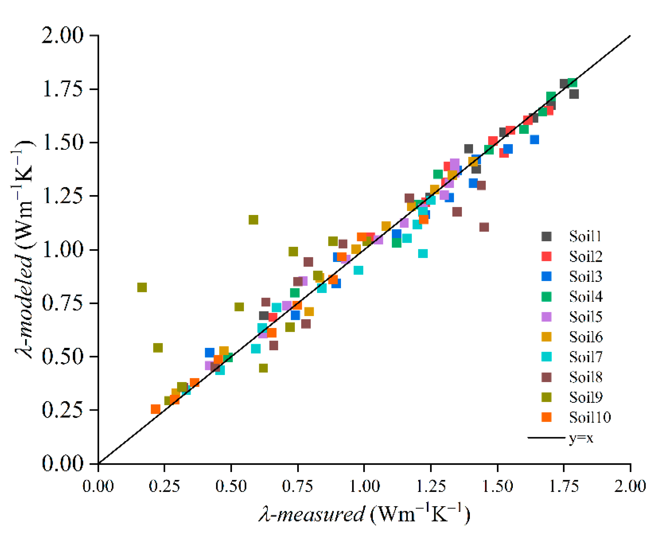
4.2.1. Model Evaluation by Laboratory Data

The comparison of soil thermal conductivity predicted by the Campbell model and the revised model that used data from the laboratory in Table 1 are as follows.

As depicted in

Table 7. Comparison of the reduced Chi-Sqr and R² of the Campbell model and the revised model on the measured soil in Table 1.

Soil Code	Reduced Chi-Sqr		R2
	Campbell	Revised	Campbell	Revised
Soil 1	0.168	0.006	0.718	0.983
Soil 2	0.178	0.012	0.803	0.982
Soil 3	0.045	0.001	0.722	0.995
Soil 4	0.077	0.002	0.782	0.988
Soil 5	0.015	0.017	0.847	0.967
Soil 6	0.022	0.002	0.84	0.987
Soil 7	0.032	0.018	0.871	0.965
Soil 8	0.073	0.004	0.792	0.991
Soil 9	0.254	0.133	0.616	0.538
Soil 10	0.045	0.002	0.912	0.981

, for other soils except Soil 9, compared with the Campbell model, the R² of the revised model is 0.001–0.012, which was much lower than 0.28–0.93 from the reduced Chi-Sqr of the original Campbell model. The R² values of the revised model are all >0.95, except for Soil 9. Soil 9 is clay loam with 0.244% salinity. The cause of this error would be the high value of the clay fraction [55]. Noborio and Mcinnes [36] suggested that clay particles interacted with salt, thereby affecting the soil’s thermal conductivity.

Figure 5 shows that the measured values of other soils except Soil 9 and the predicted thermal conductivities of the revised model with the same water content are evenly distributed on both sides of the 1:1 line, that means the revised model has good predictions on laboratory data.

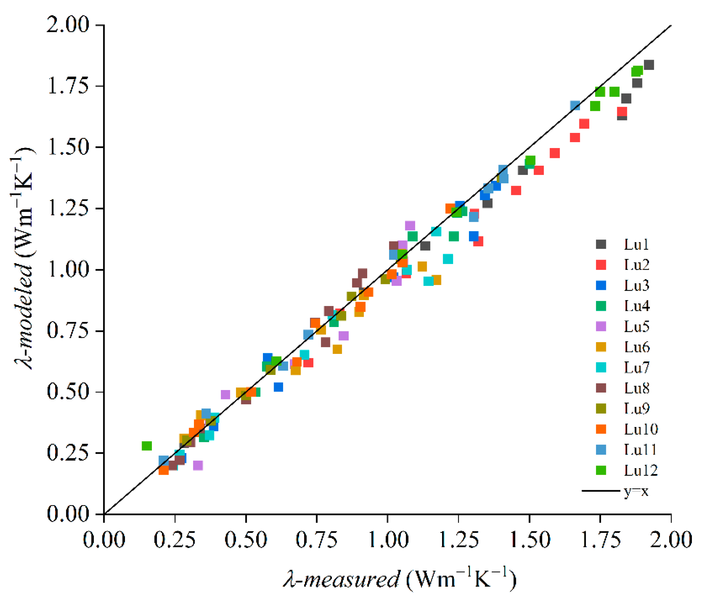
4.2.2. Model Evaluation by Data from Previous Studies

Twelve groups of data from Lu et al. [56], were used to evaluate the improved model (Figure 6).

As shown in

Table 8. Comparison of the reduced Chi-Sqr and R² of the Campbell model and the new model on the measured soil from Lu et al.

Soil Code	Type of Soil	Texture			Organic Matter	Bulk Density	Reduced Chi-Sqr		R2
		Sand	Silt	Clay
		%				g cm−3	Campbell	Revised	Campbell	Revised
Lu1	Sand	94	1	5	0.09	1.60	0.209	0.013	0.713	0.962
Lu2	Sand	93	1	6	0.07	1.60	0.202	0.017	0.782	0.872
Lu3	Sandy loam	67	21	12	0.86	1.39	0.060	0.006	0.741	0.976
Lu4	Loam	40	49	11	0.49	1.30	0.066	0.002	0.629	0.987
Lu5	Silt loam	27	51	22	1.19	1.33	0.022	0.006	0.844	0.956
Lu6	Silt loam	11	70	19	0.84	1.31	0.055	0.010	0.397	0.893
Lu7	Silty clay loam	19	54	27	0.39	1.30	0.016	0.009	0.898	0.945
Lu8	Silty clay loam	8	60	32	3.02	1.30	0.011	0.003	0.869	0.967
Lu9	Clay loam	32	38	30	0.27	1.29	0.004	0.000	0.969	0.997
Lu10	Silt loam	2	73	25	4.4	1.20	0.007	0.001	0.940	0.988
Lu11	Loam	50	41	9	0.25	1.38	0.082	0.002	0.670	0.993
Lu12	Sand	92	7	1	0.6	1.58	0.232	0.009	0.401	0.976

, for soil from previous studies, the reduced Chi-Sqr of the improved model was significantly smaller than that of the Campbell model. The measured soil thermal conductivities are evenly distributed on both sides of the 1:1 line. Moreover, the R² of the revised model is mostly >0.95. Among them, the R² of Lu 2 and Lu 6 were 0.872 and 0.893, respectively. It is assumed that these errors came from either the measurement process or interference in the salt content of the soil samples. However, their R² are still higher than those of the Campbell model, which improves the matching accuracy to a certain extent.

5. Conclusions

This study proposed a revised model of the relationship between soil water and thermal conductivity. The influence of soil texture, bulk density, and organic matter content on the λ~θ model was analyzed and the parameters that need to be improved which influenced the performance of the Campbell model were well evaluated.

Both laboratory and literature data proved that the revised model improved the accuracy of λ~θ relationship prediction and expanded the applicability of the model. However, this study was a laboratory experiment, completed by preparing soil samples, and the measurement of actual soil moisture generally requires in situ measurement. Whether the improved model can be used in in situ measurement needs further verification. The results also confirm that the revised model could not match the clay soil with a high salt concentration, which could be attributed to the interaction between clay and salt. However, for most texture and salt concentrations of soil, the revised model had higher accuracy and a wider applicable water content range than the original model. Moreover, although the revised model had improved accuracy, the calculation became more complicated and each parameter required a large amount of soil information. In the actual application process, it is necessary to use software, such as Matlab, to insert the model in the water monitoring system. The revised model is expected to provide greater service when applied to agricultural field water measurement to accurately obtain field water conditions, thereby increasing the irrigation water utilization coefficient.

References

1. Forouzani, M.; Karami, E. Agricultural water poverty index and sustainability. Agron. Sustain. Dev. 2010, 31, 415–431. [Google Scholar] [CrossRef] [Green Version]
2. Koech, R.; Langat, P. Improving Irrigation Water Use Efficiency: A Review of Advances, Challenges and Opportunities in the Australian Context. Water 2018, 10, 1771. [Google Scholar] [CrossRef] [Green Version]
3. Velasco-Muñoz, J.F.; Aznar-Sánchez, J.A.; Batlles-Delafuente, A.; Fidelibus, M.D. Sustainable Irrigation in Agriculture: An Analysis of Global Research. Water 2019, 11, 1758. [Google Scholar] [CrossRef] [Green Version]
4. Wu, P.T. The modern water-saving agricultural technology: Progress and focus. Afr. J. Biotechnol. 2010, 9, 6017–6026. [Google Scholar]
5. Ozdogan, M. Exploring the potential contribution of irrigation to global agricultural primary productivity. Glob. Biogeochem. Cycles 2011, 25. [Google Scholar] [CrossRef]
6. Xiang, K.; Li, Y.; Horton, R.; Feng, H. Similarity and difference of potential evapotranspiration and reference crop evapotranspiration—A review. Agric. Water Manag. 2020, 232, 106043. [Google Scholar] [CrossRef]
7. Hashem, M.; Qi, X. Treated Wastewater Irrigation—A Review. Water 2021, 13, 1527. [Google Scholar] [CrossRef]
8. Hatamkhani, A.; Moridi, A. Optimal Development of Agricultural Sectors in the Basin Based on Economic Efficiency and Social Equality. Water Resour. Manag. 2021, 35, 917–932. [Google Scholar] [CrossRef]
9. Hatamkhani, A.; Moridi, A. Multi-Objective Optimization of Hydropower and Agricultural Development at River Basin Scale. Water Resour. Manag. 2019, 33, 4431–4450. [Google Scholar] [CrossRef]
10. Medici, L.; Reinert, F.; de Carvalho, D.F.; Kozak, M.; Azevedo, R.A. What about keeping plants well watered? Environ. Exp. Bot. 2014, 99, 38–42. [Google Scholar] [CrossRef]
11. Wang, J.; He, H.; Li, M.; Dyck, M.; Si, B.; Lv, J. A review and evaluation of thermal conductivity models of saturated soils. Arch. Agron. Soil Sci. 2021, 67, 974–986. [Google Scholar] [CrossRef]
12. Wang, H.; Liu, C.; Zhang, L. Water-saving agriculture in China: An overview. In Advances in Agronomy; Sparks, D.L., Ed.; Elsevier BV: Amsterdam, The Netherlands, 2002; Volume 75, pp. 135–171. [Google Scholar]
13. Patle, G.T.; Kumar, M.; Khanna, M. Climate-smart water technologies for sustainable agriculture: A review. J. Water Clim. Chang. 2020, 11, 1455–1466. [Google Scholar] [CrossRef]
14. Regulwar, D.G.; Gurav, J.B. Sustainable Irrigation Planning with Imprecise Parameters under Fuzzy Environment. Water Resour. Manag. 2012, 26, 3871–3892. [Google Scholar] [CrossRef]
15. Qin, P.-J.; Liu, Z.-R.; Lai, X.-L.; Wang, Y.-B.; Song, Z.-W.; Miao, C.-X. A New Method to Determine the Spatial Sensitivity of Time Domain Reflectometry Probes Based on Three-Dimensional Weighting Theory. Water 2020, 12, 545. [Google Scholar] [CrossRef] [Green Version]
16. Hupet, F.; Vanclooster, M. Intraseasonal dynamics of soil moisture variability within a small agricultural maize cropped field. J. Hydrol. 2002, 261, 86–101. [Google Scholar] [CrossRef]
17. Ochsner, T.; Cosh, M.; Cuenca, R.H.; Dorigo, W.; Draper, C.; Hagimoto, Y.; Kerr, Y.H.; Larson, K.; Njoku, E.G.; Small, E.; et al. State of the Art in Large-Scale Soil Moisture Monitoring. Soil Sci. Soc. Am. J. 2013, 77, 1888–1919. [Google Scholar] [CrossRef] [Green Version]
18. de Vries, D. The Thermal Conductivity of Soil; North-Holland Publ. Co.,: Amsterdam, The Netherlands, 1952. [Google Scholar]
19. Johansen, O. Thermal Conductivity of Soils. Ph.D. Thesis, Norwegian University of Science and Technology, Trondheim, Norway, 1977. [Google Scholar]
20. Campbell, G.S. Soil physics with basic. In Transport Models for Soil-Plant Systems; Elsevier Sci. Publ. Co.,: New York, NY, USA, 1985. [Google Scholar]
21. Tarnawski, V.R.; Momose, T.; McCombie, M.; Leong, W.H. Canadian Field Soils III. Thermal-Conductivity Data and Modeling. Int. J. Thermophys. 2015, 36, 119–156. [Google Scholar] [CrossRef]
22. Côté, J.; Konrad, J.-M. A generalized thermal conductivity model for soils and construction materials. Can. Geotech. J. 2005, 42, 443–458. [Google Scholar] [CrossRef]
23. Flint, A.L.; Campbell, G.S.; Ellett, K.M.; Calissendorff, C. Calibration and Temperature Correction of Heat Dissipation Matric Potential Sensors. Soil Sci. Soc. Am. J. 2002, 66, 1439–1445. [Google Scholar] [CrossRef]
24. Gee, G.W.; Campbell, M.D.; Campbell, G.S.; Campbell, J.H. Rapid Measurement of Low Soil Water Potentials Using a Water Activity Meter. Soil Sci. Soc. Am. J. 1992, 56, 1068–1070. [Google Scholar] [CrossRef]
25. Marek, G.W.; Marek, T.H.; Heflin, K.R.; Porter, D.O.; Moorhead, J.E.; Schwartz, R.C.; Brauer, D.K. Factory-Calibrated Soil Water Sensor Performance Using Multiple Installation Orientations and Depths. Appl. Eng. Agric. 2020, 36, 39–54. [Google Scholar] [CrossRef]
26. Steele-Dunne, S.C.; Rutten, M.M.; Krzeminska, D.M.; Hausner, M.; Tyler, S.W.; Selker, J.; Bogaard, T.; van de Giesen, N. Feasibility of soil moisture estimation using passive distributed temperature sensing. Water Resour. Res. 2010, 46. [Google Scholar] [CrossRef] [Green Version]
27. Sayde, C.; Gregory, C.; Gil-Rodriguez, M.; Tufillaro, N.; Tyler, S.; van de Giesen, N.; English, M.; Cuenca, R.; Selker, J. Feasibility of soil moisture monitoring with heated fiber optics. Water Resour. Res. 2010, 46. [Google Scholar] [CrossRef] [Green Version]
28. Kaveh, M.; Keyvan, M.; Fahimeh, K. Response of soil thermal conductivity to various soil properties. Int. Commun. Heat Mass Transf. 2021, 127, 105516. [Google Scholar]
29. Sadeghi, M. Comment on “A model for soil surface evaporation based on Campbell’s retention curve” by G. Zarei, M. Homaee, A.M. Liaghat, A.H. Hoorfar. J. Hydrol. 2015, 525, 486–488. [Google Scholar] [CrossRef]
30. Wierenga, P.J.; Nielsen, D.R.; Hagan, R.M. Thermal Properties of a Soil Based Upon Field and Laboratory Measurements. Soil Sci. Soc. Am. J. 1969, 33, 354–360. [Google Scholar] [CrossRef]
31. Usowicz, B.; Lipiec, J. The effect of exogenous organic matter on the thermal properties of tilled soils in Poland and the Czech Republic. J. Soils Sediments 2020, 20, 365–379. [Google Scholar] [CrossRef] [Green Version]
32. Lipiec, J.; Hatano, R. Quantification of compaction effects on soil physical properties and crop growth. Geoderma 2003, 116, 107–136. [Google Scholar] [CrossRef]
33. Bachmann, J.; Horton, R.; Ren, T.; Van Der Ploeg, R.R. Comparison of the thermal properties of four wettable and four water-repellent soils. Soil Sci. Soc. Am. J. 2001, 65, 1675–1679. [Google Scholar] [CrossRef]
34. Su, L.; Wang, Q.; Wang, S.; Wang, W. Soil thermal conductivity model based on soil physical basic parameters. Trans. Chin. Soc. Agric. Eng. 2016, 32, 127–133. [Google Scholar]
35. Mahdavi, S.M.; Neyshabouri, M.R.; Fujimaki, H. Assessment of some soil thermal conductivity models via variations in temperature and bulk density at low moisture range. Eurasian Soil Sci. 2016, 49, 915–925. [Google Scholar] [CrossRef]
36. Noborio, K.; Mcinnes, K.J. Thermal Conductivity of Salt-Affected Soils. Soil Sci. Soc. Am. J. 1993, 57, 329. [Google Scholar] [CrossRef]
37. Wallen, B.M.; Smits, K.; Sakaki, T.; Howington, S.E.; Chamindu Deepagoda, T.K.K. Thermal Conductivity of Binary Sand Mixtures Evaluated through Full Water Content Range. Soil Sci. Soc. Am. J. 2016, 80, 592–603. [Google Scholar] [CrossRef]
38. Zhao, B.; Li, L.; Zhao, Y.; Zhang, X. Thermal conductivity of a Brown Earth soil as affected by biochars derived at different temperatures: Experiment and prediction with the Campbell model. Int. Agrophys. 2020, 34, 433–439. [Google Scholar] [CrossRef]
39. Li, T.; Wang, Q.; Fan, J. Modification and comparison of methods for determining soil thermal parameters. Trans. Chin. Soc. Agric. Eng. 2008, 24, 59–64. [Google Scholar]
40. Abu-Hamdeh, N.H.; Reeder, R.C. Soil Thermal Conductivity Effects of Density, Moisture, Salt Concentration, and Organic Matter. Soil Sci. Soc. Am. J. 2000, 64, 1285–1290. [Google Scholar] [CrossRef]
41. Indorante, S.J.; Hammer, R.D.; Koenig, P.G.; Follmer, L.R. Particle-Size Analysis by a Modified Pipette Procedure. Soil Sci. Soc. Am. J. 1990, 54, 560–563. [Google Scholar] [CrossRef]
42. Jacobsen, O.; Schjønning, P. A laboratory calibration of time domain reflectometry for soil water measurement including effects of bulk density and texture. J. Hydrol. 1993, 151, 147–157. [Google Scholar] [CrossRef]
43. Vitti, C.; Stellacci, A.M.; Leogrande, R.; Mastrangelo, M.; Cazzato, E.; Ventrella, D. Assessment of organic carbon in soils: A comparison between the Springer–Klee wet digestion and the dry combustion methods in Mediterranean soils (Southern Italy). Catena 2016, 137, 113–119. [Google Scholar] [CrossRef]
44. Fujimaki, H.; Shiozawa, S.; Inoue, M. Effect of salty crust on soil albedo. Agric. For. Meteorol. 2003, 118, 125–135. [Google Scholar] [CrossRef]
45. Burland, B.J. On the compressibility and shear strength of natural clays. Geotechnique 1990, 40, 329–378. [Google Scholar] [CrossRef]
46. Farouki, O.T. The thermal properties of soils in cold regions. Cold Reg. Sci. Technol. 1981, 5, 67–75. [Google Scholar] [CrossRef]
47. Lawrence, D.M.; Slater, A.G. Incorporating organic soil into a global climate model. Clim. Dyn. 2008, 30, 145–160. [Google Scholar] [CrossRef]
48. Gamage, D.N.V.; Biswas, A.; Strachan, I.B. Spatial variability of soil thermal properties and their relationships with physical properties at field scale. Soil Tillage Res. 2019, 193, 50–58. [Google Scholar] [CrossRef]
49. Mengistu, A.G.; Van Rensburg, L.D.; Mavimbela, S.S. The effect of soil water and temperature on thermal properties of two soils developed from aeolian sands in South Africa. Catena 2017, 158, 184–193. [Google Scholar] [CrossRef]
50. Cegła, M.; Zmywaczyk, J.; Koniorczyk, P. Alternative method of determination of thermo-physical properties of energetic materials. In Proceedings of the 23rd International Meeting of Thermophysics, Smolenice, Slovakia, 7–9 November 2018. [Google Scholar]
51. Menard, S. Coefficients of Determination for Multiple Logistic Regression Analysis. Am. Stat. 2000, 54, 17. [Google Scholar] [CrossRef]
52. Zhang, Y.-B.; Li, D.-J.; Yan, H.-J.; Zhao, J. Estimation for the Moisture Content of Oil-immersed Insulating Pressboard Using Dielectric Characteristic Parameter. In Proceedings of the 2nd International Conference on Electrical and Electronic Engineering (EEE 2019), Hangzhou, China, 26–27 May 2019. [Google Scholar]
53. Tarnawski, V.R.; McCombie, M.L.; Leong, W.H.; Wagner, B.; Momose, T.; Schönenberger, J. Canadian Field Soils II. Modeling of Quartz Occurrence. Int. J. Thermophys. 2012, 33, 843–863. [Google Scholar] [CrossRef]
54. Andrady, A.L. Microplastics in the marine environment. Mar. Pollut. Bull. 2011, 62, 1596–1605. [Google Scholar] [CrossRef]
55. Cao, Y. Study on the Model and Errors in Data Fitting. In Proceedings of the International Conference on Informatization in Education, Management and Business (IEMB), Guangzhou, China, 13–14 September 2014. [Google Scholar]
56. Lu, S.; Ren, T.; Gong, Y.; Horton, R. An Improved Model for Predicting Soil Thermal Conductivity from Water Content at Room Temperature. Soil Sci. Soc. Am. J. 2007, 71, 8–14. [Google Scholar] [CrossRef]
Figure 1. The measured relationship of λ~θ and the curves estimated by the Campbell model for soil with different textures. The colored dots represent the measured values and the dotted lines represent the Campbell model curves.
Water 13 03441 g001
Figure 2. The measured relationship of λ~θ and the curves estimated by the Campbell model for soil with different bulk densities. The colored dots represent the measured values and the dotted lines represent the Campbell model curves.
Water 13 03441 g002
Figure 3. The relationship of λ~θ and the curve estimated by the Campbell model for soil with different organic matter contents. Figure (a) shows the results of Soil 1, representing sandy soil. Figure (b) shows the results of Soil 10, representing clay soil.
Water 13 03441 g003
Figure 4. The influence of m and E values on the shape of the λ~θ curve, respectively. Figure (a) shows the influence of different values of m on the curve when E = 0.8 and Figure (b) shows the influence of different values of E on the curve when m = 0.7.
Water 13 03441 g004
Figure 5. Comparison of predicted soil thermal conductivity (λ) values from the new model vs. measured data under the same water content of soils in Table 1.
Water 13 03441 g005
Figure 6. Comparison of soil thermal conductivity predicted from the revised model vs. measured values.
Water 13 03441 g006