Article

Case Study of Urban Flood Inundation—Impact of Temporal Variability in Rainfall Events

1
School of Architectural, Civil, Environmental and Energy Engineering, Kyungpook National University, 80 Daehak-ro, Buk-gu, Daegu 41566, Korea
2
Center for Atmospheric REmote Sensing (CARE), Department of Astronomy and Atmospheric Sciences, Kyungpook National University, 80 Daehak-ro, Buk-gu, Daegu 41566, Korea
*
Author to whom correspondence should be addressed.
Water 2021, 13(23), 3438; https://doi.org/10.3390/w13233438
Submission received: 3 November 2021 / Revised: 30 November 2021 / Accepted: 1 December 2021 / Published: 4 December 2021
(This article belongs to the Topic Water Management in the Era of Climatic Change)

Abstract

:
This study aimed to calculate and analyze total overflows that accumulate in urban manholes in the target drainage basin of Samsung-dong, Seoul in heavy rainfall events with different temporal distribution characteristics, using the EPA’s Storm Water Management Model (EPA-SWMM model). Inundation behaviors were analyzed using the two-dimensional flood model (FLO-2D). The extreme rainfall events were produced using different exceedance probability Huff distributions for different durations and return periods, such as from 1 to 3 h and 10 years, 50 years, 80 years, 100 years, respectively. The inundation model was validated using the actual flood observations on 21 September 2010 in the Samsung-dong drainage basin. The total overflow amount showed considerable differences according to the different time distribution characteristics, such as the temporal location of the storm peak and the concentration level of the storm. Furthermore, the inundation behaviors were also related to the temporal characteristics of storms. The results illustrated that the consideration of the temporal distribution characteristics of extreme rainfall events is essential for an accurate understanding of the rainfallrunoff response and inundation behavior in urban drainage basins.

1. Introduction

The issue of urban flood inundation has become a key global concern in recent years because of the regional impacts of climate change, which cause more frequent short-duration extreme storms [1]. The negative impacts of urban floods include the failure of city infrastructure, economic loss, the risk to life, etc. Inundation in urban areas is associated not only with the increase in the intensity and frequency of extreme rainfall, but also with impermeable surfaces and limited discharge capacity during heavy rainfall, as well as inappropriate artificial interventions that affect the intensity and magnitude of floods [2,3,4]. Analyses of the temporal characteristics of rainfall in Korea show a gradual increase in the intensity and frequency of extreme rainfall events. Therefore, the failure of the stormwater drainage system has become more frequent and severe. The metropolitan area of Seoul is vulnerable to urban flooding due to its high precipitation compared to other regions of Korea [5,6]. Recently, the potential for flood-resilient and sustainable redevelopment of Seoul was analyzed to propose city renovation strategies for resistance to flood disasters [7]. In Japan, urban flood vulnerability was quantified by analyzing the topographic characteristics of a fluvial area of the Kaki River in Nagaoka city to evaluate evacuation urgency during urban flooding [8]. Various studies have been conducted to accurately express the temporal distribution characteristics of input rainfall data used for urban flood simulation and analysis, including the Keifer and Chu method [9], the method suggested by Yen and Chow [10], the SCS curve method [11], the Huff method [12], etc. For example, the SCS curve method has been used in urban areas to predict the surface runoff from impervious areas and sediment yield in downstream areas [13]. In South Korea, there have been many studies on the distribution of Huff rainfall time; the Huff rainfall distribution is constructed so that the peak of the heavy rain can be placed in the desired time section. This tends to represent the time distribution of heavy rain relatively well; therefore, the Huff method was chosen in this study as the time distribution of rainfall was suitable for the applied rainfall–runoff model [14].
Many studies have been conducted on the assessment and management of urban flood inundation, using the Huff method to represent the time distribution of heavy storms. Yang et al. [15] modeled floods by coupling the 1D stormwater management model (SWMM) and the 2D flood inundation model (ECNU Flood-Urban) to analyze rainfall–runoff processes in an urban environment in the central business district of East Nanjing Road in downtown Shanghai. Bezak et al. [16] investigated the impact of the different design rainfall events of Huff curves on the combined 1D/2D hydraulic modeling results. Lee [17] proposed a support plan for the Huff rainfall distribution, impact-based, urban flooding forecast. The SWMM or FLO-2D models can be used to predict floods and pipeline drainage, or prepare flood hazard maps. Erena et al. [18] proposed local flood management strategies for 232 households located in flood-prone areas of Dire Dawa city, Ethiopia. Flood hazard mapping was used for different storm events. Luo et al. [19] used a calibrated flood inundation model to assess the influence of four extreme rainfall events on water depth and inundation area in the Hanoi Central Area, Vietnam. The research only focused on overland flooding caused by extreme rainfall, while little attention was paid to floods caused by failures of the drainage system. Vojtek et al. [20] investigated the sensitivity of flood areas, flood volume associated with model input parameters, and showed the importance of proper input parameter estimation in the flood simulation. GebreEgziabher et al. [21] coupled the one-dimensional SWMM model with the new flood inundation and recession model (FIRM) to model urban flood inundation and recession and the impact of manhole characteristics such as spatial extent and depth.
Urban floods are highly associated not only with future rainfall quantities, but also the time distribution characteristics of heavy storms, the antecedent rainfall conditions, the capacity of drainage networks, etc. Among all of these factors, the influence of the temporal patterns of extreme rainfall on the manhole overflow is one of the most important factors. Previous research has demonstrated that the impacts of the temporal characteristics of potential extreme rainfall events on the amount of urban flooding should be considered to enhance urban flood risk management systems. Nevertheless, previous studies have not thoroughly explored the impacts of the time distribution characteristics of extreme rainfall patterns on urban floods.
The temporal concentration level of storms and the storm peak occurrence quartile are the main time distribution characteristics of heavy storms associated with manhole overflow. In this study, the urban flood inundation impacts caused by the temporal concentration level of storms and the storm peak occurrence quartile were analyzed for a target drainage basin in Seoul, Korea. The total manhole overflow in the target urban drainage basin was calculated using the EPA-SWMM model for different rainfall scenarios. Rainfall scenarios reflecting the temporal characteristics of rainfall events were constructed using the Huff method. The impacts of the temporal concentration level were analyzed using nine different exceedance probabilities (10–90%) and the impacts of the temporal location of storm peak were analyzed using four different quartiles (1–4th quartile) for three different storm durations (1–3 h) and four different return periods (10, 50, 80, and 100-years). The two-dimensional inundation analysis of the overflow in each manhole was conducted using the FLO-2D model.

2. Materials and Methods

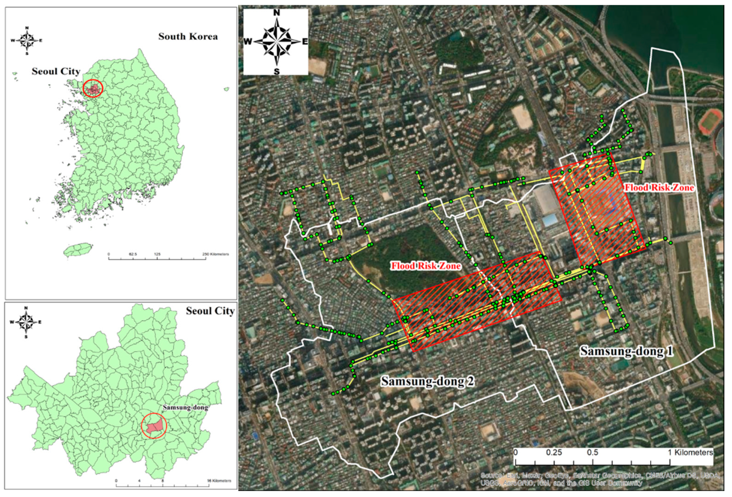
2.1. Study Area and Input Rainfall Data

The Samsung-dong area is divided into Samsung 1-dong and Samsung 2-dong, and is located in the Seoul metropolitan area, which contains 239 drainage basins. Samsung-dong has a population of 44,031, with an area of 3.18 km2, and there are 342 manholes and 359 conduit links from the urban drainage system in the study area. Rainwater from both areas is pumped to the Tancheon river (Figure 1). The ratio of the impervious area in Seoul is as high as 54.4% according to the management report of the National Institute of Environmental Sciences of Korea, 2014. Samsung-dong, which is a part of Gangnam-gu, Seoul, consists of relatively low land and has a complex drainage system. Figure 2 showed the actual rainfall on 21 September 2010 which was used for the verification of the EPA-SWMM and FLO-2D model and extreme rainfall scenario using the Huff time distribution method which were used for analysis. An inundation trace map shows the extent of flooding from rainfall on 21 September 2010 (Figure 3) [22].
For more accurate research on the impact of extreme rainfall on severe flooding in the city, the latest precipitation data from an automated synoptic observing system (ASOS) were obtained from the South Korea Meteorological Administration. The actual rainfall on 21 September 2010 was investigated, and the Huff method produced data for different duration periods of extreme rainfall; the total extreme rainfall event data included 432 different periods of extreme rainfall event data, such as 10-year, 50-year, 80-year, and 100-year periods. The Huff curve characterizes the temporal distribution of rainfall depth over an area and is widely utilized as an input to rainfall–runoff models for drainage design [23,24]. Most urban floods occur within 6 h, and the duration of extreme rainfall is divided into 1-h, 2-h, and 3-h timespans [25]. Table 1 shows the total, maximum and minimum rainfall during five extreme rainfall periods. Figure 2 shows that the actual total rainfall was 278 mm, minimum rainfall was 1 mm and maximum rainfall was 19 mm on 21 September 2010, with representative changes over 6 h of extreme rainfall event data.

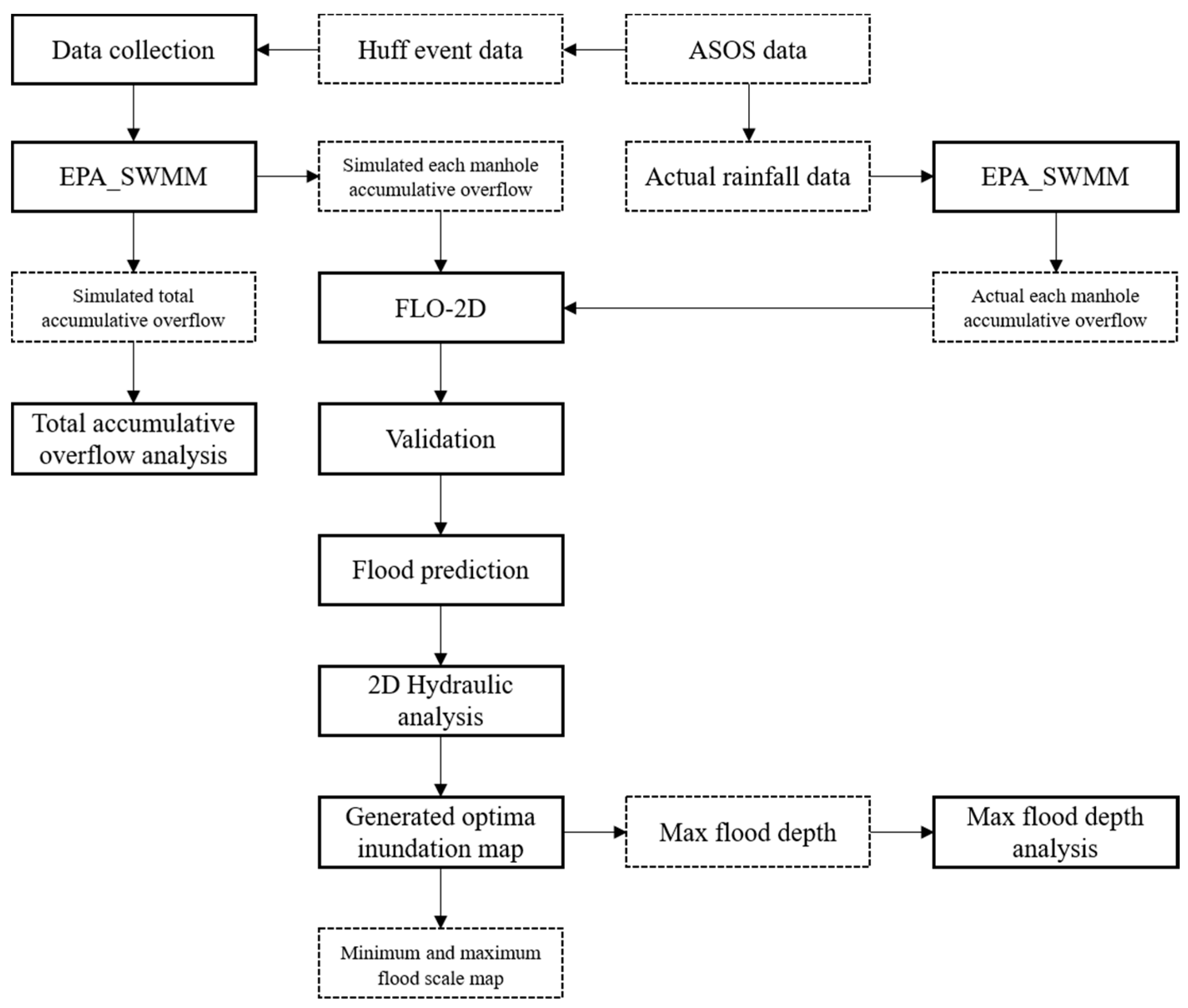
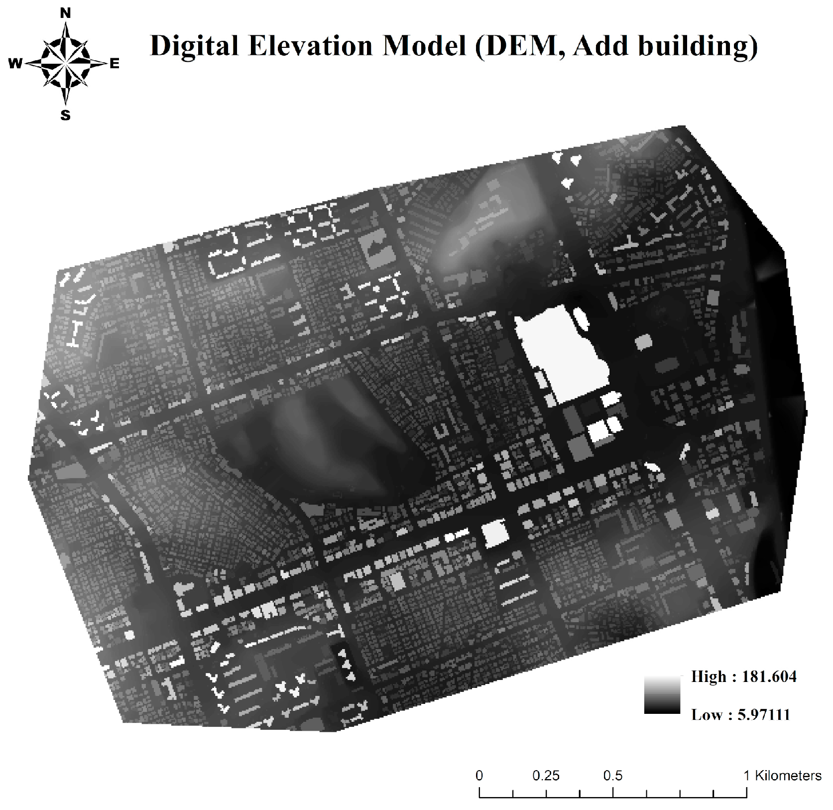
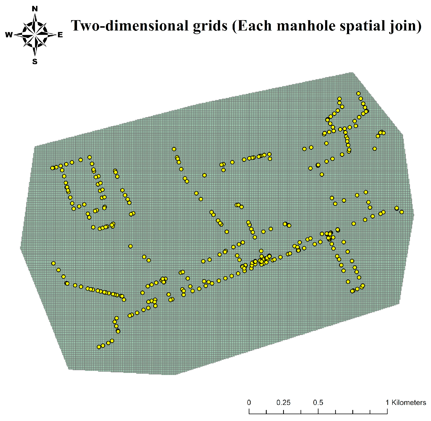
2.2. Hydraulic Modeling (EPA-SWMM and FLO-2D Model)

To construct the flood prediction model and calculate the runoff or overflow at each manhole in the urban watershed, the EPA-SWMM model was used to simulate 432 different extreme rainfall event data (1 to 3-h, in 10 min intervals) considering the high-intensity rainfall conditions. This was obtained from the United States Environmental Protection Agency and was useful for checking the amount of urban overflow [26]. The EPA-SWMM can calculate the total accumulative overflow in the study area. The flood volume for each rainfall scenario was calculated and the flows in the drainage pipe network in urban basins with drainage systems were analyzed [27]. The EPA-SWMM model performed the initial calculations of the flow rate and depth of the drainage pipe system, which allowed analysis of the backflow and overflow amount in the pipe based on the various rainfall events in the study area [28]. The Saint–Venant equations (Equations (1) and (2)) were used in this calculation.
Q = W × 1 n ( d d p ) 5 3 × S 1 2
Q t + g A S f 2 V A t V 2 A x + g A H x = 0
where Q is runoff (m3/s), W is the sub-watershed width (m), n is the Manning’s roughness coefficient, d is the depth (m), dp is the ground reservoir lost depth (m), S is the sub-watershed slope, A is the surface flow cross-sectional area of sub-watershed (m2), and V is the surface flow velocity (m/s). The EPA-SWMM model was used for the one-dimensional simulation of urban flood overflow analysis. To determine the adequacy of the one-dimensional urban runoff analysis results, the total accumulative overflow at each manhole point underwent a two-dimensional inundation analysis using a two-dimensional flood analysis program, the FLO-2D model [29]. The results were compared with those for actual flood areas because only the actual flood map can be used to verify the EPA-SWMM-simulated results at present, and data on the water level and discharge in the conduit were absent. Figure 3 shows the verification of the two-dimensional flood analysis results used for rainfall data and the flood mask map from 21 September 2010 in Samsung-dong. The total rainfall was 278 mm over 6 h in 10 min intervals.
FLO-2D is a grid-based, two-dimensional hydraulic model approved by the Federal Emergency Management Agency (FEMA), and developed by O’Brien in 2003. It is a two-dimensional, finite-difference model used to simulate flood hazards and urban floodplains [30]. In the whole digital elevation model simulated domain, the construction of two-dimensional grids needs to be completed; the exact location of a manhole in the two-dimensional 5 m2 grid system was found by using the spatial join tool of the ArcGIS model and flood routing and two-dimensional inundation analysis were performed using the FLO-2D model. Interactive flood routing between channel, street, and floodplain flow was performed using a 5 m2 grid system to properly reflect the influence of buildings and roads on the flood waves, and to describe the complex floodplain topography. The overflows of each manhole were calculated from EPA-SWMM, and these were entered into the input file of FLO-2D, which helped construct the two-dimensional grids. After completing the two-dimensional grids, the model-governing equations included the continuity equation and the two-dimensional equations of motion. The one continuity equation (Equation (3)) and two momentum equations were applied in the x and y directions (Equations (4) and (5), respectively) to carry out a two-dimensional analysis of urban flood inundation changes [31,32]. According to the results compared with those for actual flood areas, the synthetic roughness coefficient calibrated was 0.15.
d t + q x x + q y   y = e
u t + u u x + v u y = g ( S o x S f x d x )
v t + u v x + v v y = g ( S o y S f y d y )
where d is depth at a surface; qx and qy are the flows per unit width in the x and y directions, respectively; u and v indicate average velocities in the x and y directions, respectively; Sox and Soy are the bed slope x and y directions, respectively; Sfx and Sfy are the friction slopes in the x and y directions, respectively. The variable e is the generation or extinction section per unit area.
Figure 4 illustrates the summarized procedure of the EPA-SWMM and FLO-2D simulation. To effectively calculate and analyze total overflows that accumulated in urban manholes with different temporal distribution characteristics, heavy rainfall scenarios were designed using the Huff rainfall distribution method and the 10 min intervals rainfall data from the Seoul site of the Automated Synoptic Observation System (ASOS) of the Korea Meteorological Administration. These rainfall scenario data were used as the input for the EPA-SWMM to calculate the total overflow amount of each manhole in the target drainage basin of Samsung-dong, Seoul, Korea. The EPA-SWMM model was suitable for the one-dimensional simulation of urban flood overflow analysis. The adequacy of the one-dimensional urban runoff analysis results was validated for the actual urban flood observation by using a two-dimensional flood analysis program, the FLO-2D model. To do the two-dimensional flood simulation, a digital elevation model (DEM) (Figure 5) with a 5-m cell size was composed of the target area, which was produced by using the add building tool in the ArcGIS model.
In addition, the exact location of each manhole was found by using the spatial join tool in the ArcGIS model in the whole 5-m cell size digital elevation model simulated domain, which was needed to complete the construction of two-dimensional grids (Figure 6). After completing the two-dimensional grids, the total overflows of each manhole data and the exact location of each manhole were used as the input data for the FLO-2D model. Flood routing and two-dimensional inundation analysis were performed by interactive flood routing between channel, street, and floodplain flow to properly reflect the influence of buildings, and describe the complex floodplain topography. Also, the mapper pro. 2009 tool in the FLO-2D model was used to generate maximum flow depth in the cell map and to generate the optimal inundation map. The optimal inundation maps were generated according to the total overflows, reflecting different temporal rainfall distribution characteristics.

3. Results and Discussion

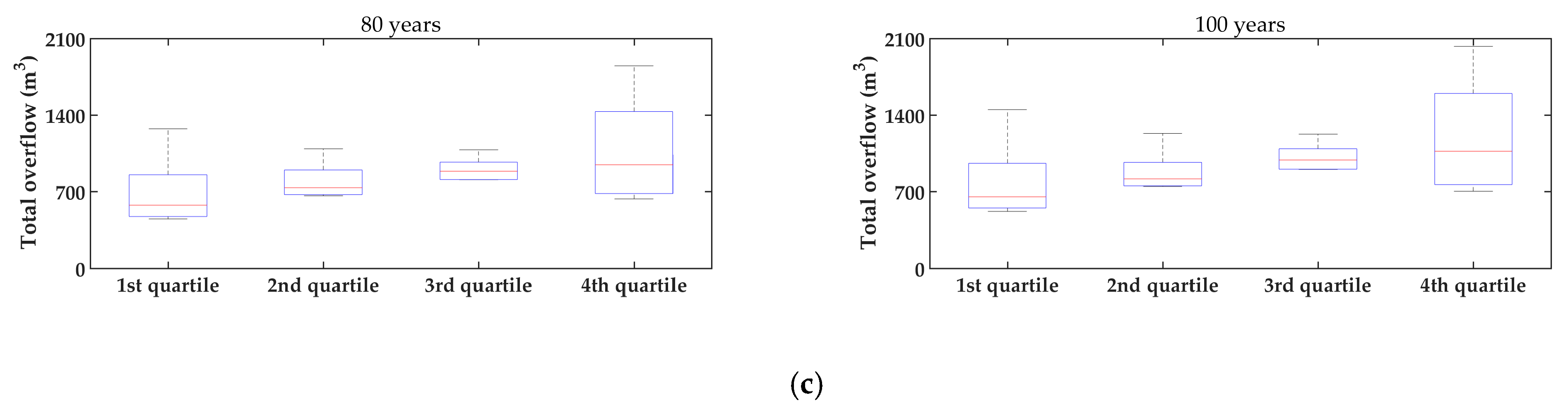
3.1. EPA-SWMM Model Simulation Results for Accumulated Manholes Overflows

The accumulated manhole overflow from 342 manholes in the study area was simulated using the EPA-SWMM model, and a model input rainfall database was established using diverse extreme rainfall events. The extreme rainfall event database periods were 10-years, 50-years, 80-years, and 100-years. The total rainfall is shown in Table 1, over 1-h, 2-h, and 3-h periods (in 10 min intervals). Table 2 shows the total EPA-SWMM-model-simulated overflow results for a duration of one hour over different periods in the same quartiles. The extreme rainfall data produced by the Huff method were used.
In a period of 10 years, the Huff method’s simulated results for the 1st quartile showed a minimum total overflow of 22.8 m3, a maximum total overflow of 110.2 m3, and an average total overflow of 61.6 m3. In a period of 50 years, the Huff method 1st quartile simulated results showed minimum, maximum and average total overflows with significant increases of 91.5 to 284.8 m3 relative to the 10-year simulated results. However, in a period of 80 years, the Huff method 1st quartile simulated results showed that the minimum, maximum and average total overflows increased by 18.1 to 94.7 m3 relative to the 50-year simulated results. In a period of 100 years, the Huff method 1st quartile simulated results showed that the minimum, maximum, and average total overflows were increased by 14.2 to 46.3 m3 relative to the 80-year simulated results. Additionally, in a period of 10 years, the Huff method 2nd quartile simulated results showed minimum, maximum and average total overflows of 74.3 m3, 102.7 m3, and 89.7 m3, respectively. In a period of 50 years, the Huff method 2nd quartile simulated results showed minimum, maximum and average total overflows with significant increases of 65.8 to 98.3 m3 relative to the 10-year simulated results. In a period of 80 years, the Huff method 2nd quartile simulated results showed that minimum, maximum and average total overflows were increased by 19.9 to 35.4 m3 relative to the 50-year simulated results. In a period of 100 years, the Huff method 2nd quartile simulated results showed that minimum, maximum and average total overflows were increased by 19.5 to 54.0 m3 relative to the 80-year simulated results. Additionally, in a period of 10 years, the Huff method 3rd quartile simulated results showed minimum, maximum and average total overflows of 71.4 m3, 115.4 m3, and 92.9 m3, respectively. In a period of 50 years, the Huff method 3rd quartile simulated results showed minimum, maximum and average total overflows with significant increases ranging from 81.5 to 90.4 m3 relative to the 10-year simulated results. However, in a period of 80 years, the Huff method 3rd quartile simulated results showed that the minimum, maximum and average total overflows increased by 25.3 to 62.3 m3 relative to the 50-year simulated results. In a period of 100 years, the Huff method 3rd quartile simulated results showed the minimum, maximum and average total overflows to be increased by 10.9 to 28.6 m3 relative to the 80-year simulated results. Finally, in a period of 10 years, the Huff method 4th quartile simulated results showed minimum, maximum and average total overflows of 43.4 m3, 133.2 m3, and 84.9 m3, respectively. In a period of 50 years, the Huff method 4th quartile simulated results showed increases in minimum, maximum and average total overflow of 70.3 to 353.6 m3 relative to the 10-year simulated results. In a period of 80 years, the Huff method 4th quartile simulated results showed minimum, maximum, and average total overflows that were increased by 25.5 to 152.3 m3 relative to the 50-year simulated results. In a period of 100 years, the Huff method 4th quartile simulated results showed minimum, maximum and average total overflows to be increased by 13.0 to 79.1 m3 relative to the 80-year simulated results.
Table 3 shows the EPA-SWMM-model-simulated overflow results for a duration of two hours. Similarly, in a period of 10 years, the Huff method 1st quartile simulated results showed minimum, maximum and average total overflows of 28.1 m3, 203.5 m3, and 101.1 m3, respectively. In a period of 50 years, the Huff method 1st quartile simulated results showed minimum, maximum and average total overflows with significant increases of 128.1 to 470.4 m3. In a period of 80 years, the Huff method 1st quartile simulated results showed minimum, maximum and average total overflows were increased by 76.7 to 247.7 m3. In a 100-year period, the Huff method 1st quartile simulated results showed the minimum, maximum, and average total overflow was increased by 42.6 to 129.0 m3. In a period of 10 years, the Huff method 2nd quartile simulated results showed minimum, maximum and average total overflows of 93.8 m3, 182.1 m3, and 141.9 m3 respectively. In a period of 50 years, the Huff method 2nd quartile simulated results showed minimum, maximum, and average total overflow with significant increases of 228.9 to 296.1 m3. In a period of 80 years, the Huff method 2nd quartile simulated results showed that the minimum, maximum and average total overflows increased by 96.0 to 177.8 m3. In a period of 100 years, the Huff method 2nd quartile simulated results showed that minimum, maximum and average total overflows increased by 40.8 to 83.1 m3. In a period of 10 years, the Huff method 3rd quartile simulated results showed minimum, maximum, and average total overflows of 121.2 m3, 201.9 m3, and 159.5 m3, respectively. In a period of 50 years, the Huff method 3rd quartile simulated results showed minimum, maximum and average total overflows with significant increases of 250.1 to 326.2 m3. In a period of 80 years, the Huff method 3rd quartile simulated results showed minimum, maximum and average total overflows to be increased by 104.3 to 124.6 m3. In a period of 100 years, the Huff method 3rd quartile simulated results showed minimum, maximum and average total overflows were increased by 46.01 to 74.6 m3. In a period of 10 years, the Huff method 4th quartile simulated results showed minimum, maximum and average total overflows of 74.3 m3, 361.5 m3, and 177.0 m3, respectively. In a period of 50 years, the Huff method 4th quartile simulated results showed minimum, maximum and average total overflows with significant increases of 181.6 to 624.2 m3. In a period of 80 years, the Huff method 4th quartile simulated results showed that the minimum, maximum and average total overflows increased by 90.5 to 281.2 m3. In a period of 100 years, the Huff method 4th quartile simulated results showed that the minimum, maximum and average total overflows increased by 47.7 to 127.3 m3.
Finally, Table 4 shows the EPA-SWMM-model-simulated results for a duration of three hours. In a period of 10 years, the Huff method 1st quartile simulated results showed minimum, maximum and average total overflows of 27.3 m3, 286.5 m3, and 123.5 m3, respectively. In a period of 50 years, the Huff method 1st quartile simulated results showed minimum, maximum and average total overflows with significant increases ranging from 271.0 to 630.8 m3. In a period of 80 years, the Huff method 1st quartile simulated results showed that minimum, maximum and average total overflows increased by 152.6 to 354.1 m3. In a period of 100 years, the Huff method 1st quartile simulated results showed that minimum, maximum and average total overflows increased by 68.4 to 176.7 m3. Similarly, in a period of 10 years, the Huff method 2nd quartile simulated results showed the minimum, maximum and average total overflows were 100.0 m3, 256.8 m3, and 166.7 m3, respectively. In a period of 50 years, the Huff method 2nd quartile simulated results showed minimum, maximum and average total overflows with significant increases of 428.2 to 544.1 m3. In a period of 80 years, the Huff method 2nd quartile simulated results showed minimum, maximum and average total overflows to be increased by 133.5 to 290.3 m3. In a period of 100 years, the Huff method 2nd quartile simulated results showed that minimum, maximum and average total overflows were increased by 77.1 to 141.7 m3. In a period of 10 years, the Huff method 3rd quartile simulated results showed minimum, maximum, and average total overflows of 174.1 m3, 371.3 m3, and 231.6 m3, respectively. In a period of 50 years, the Huff method 3rd quartile simulated results showed minimum, maximum and average total overflows with significant increases of 426.3 to 463.1 m3. In a period of 80 years, the Huff method 3rd quartile simulated results showed that minimum, maximum and average total overflows increased by 193.9 to 253.3 m3. In a period of 100 years, the Huff method 3rd quartile simulated results showed minimum, maximum and average total overflows were increased by 93.7 to 144.1 m3. In a period of 10 years, the Huff method 4th quartile simulated results showed minimum, maximum, and average total overflows of 119.5 m3, 459.9 m3, and 269.3 m3, respectively. In a period of 50 years, the Huff method 4th quartile simulated results showed minimum, maximum and average total overflows with significant increases of 349.7 to 996.7 m3. In a period of 80 years, the Huff method 4th quartile simulated results showed that minimum, maximum and average total overflows increased by 164.1 to 391.3 m3. In a period of 100 years, the Huff method 4th quartile simulated results showed minimum, maximum and average total overflows were increased by 70.1 to 179.3 m3. The simulated total overflow results for different periods in the same quantiles showed a gradual increase in simulated overflow over the different periods, with significant increases concentrated in a 50-year period.

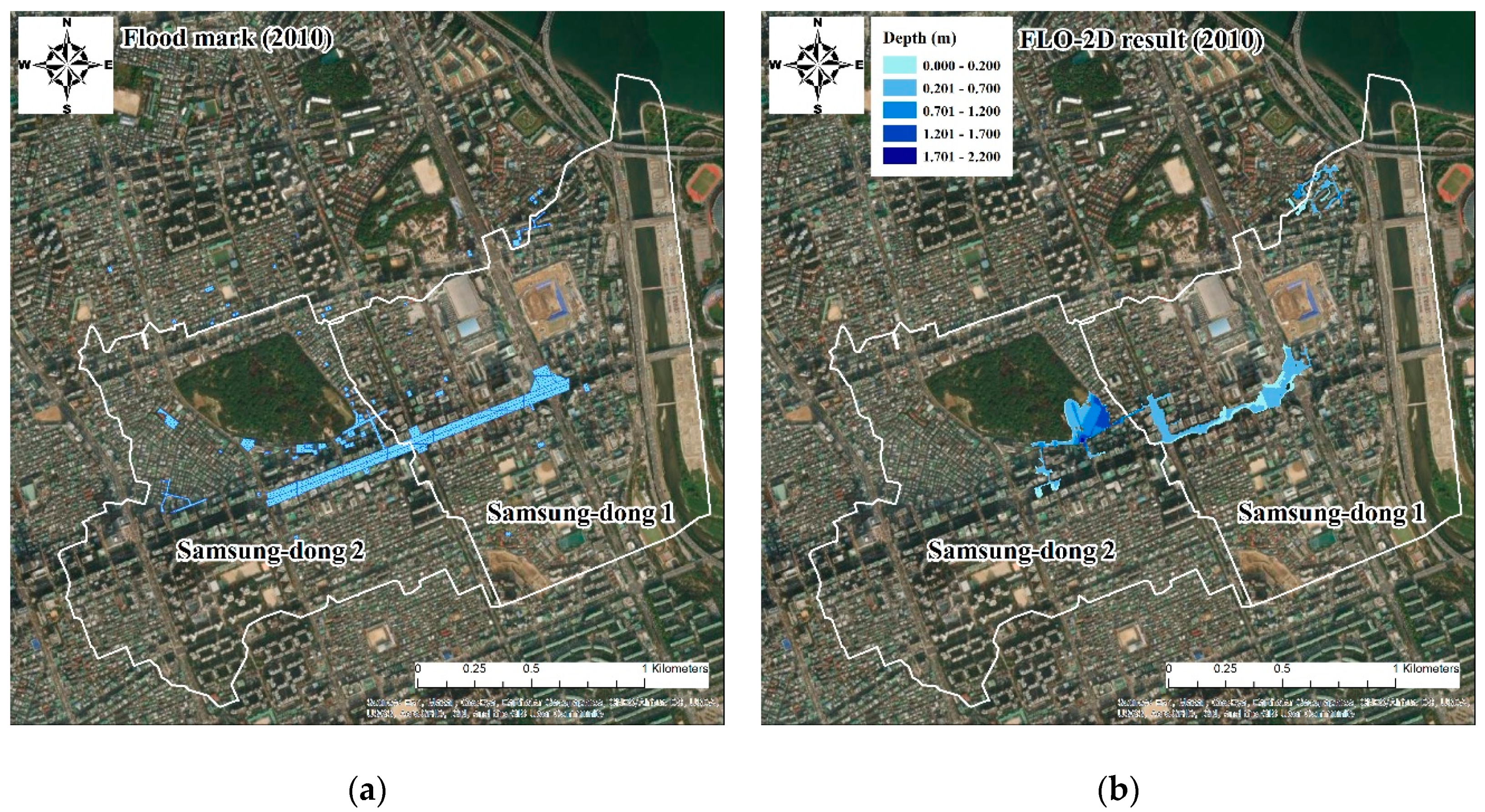
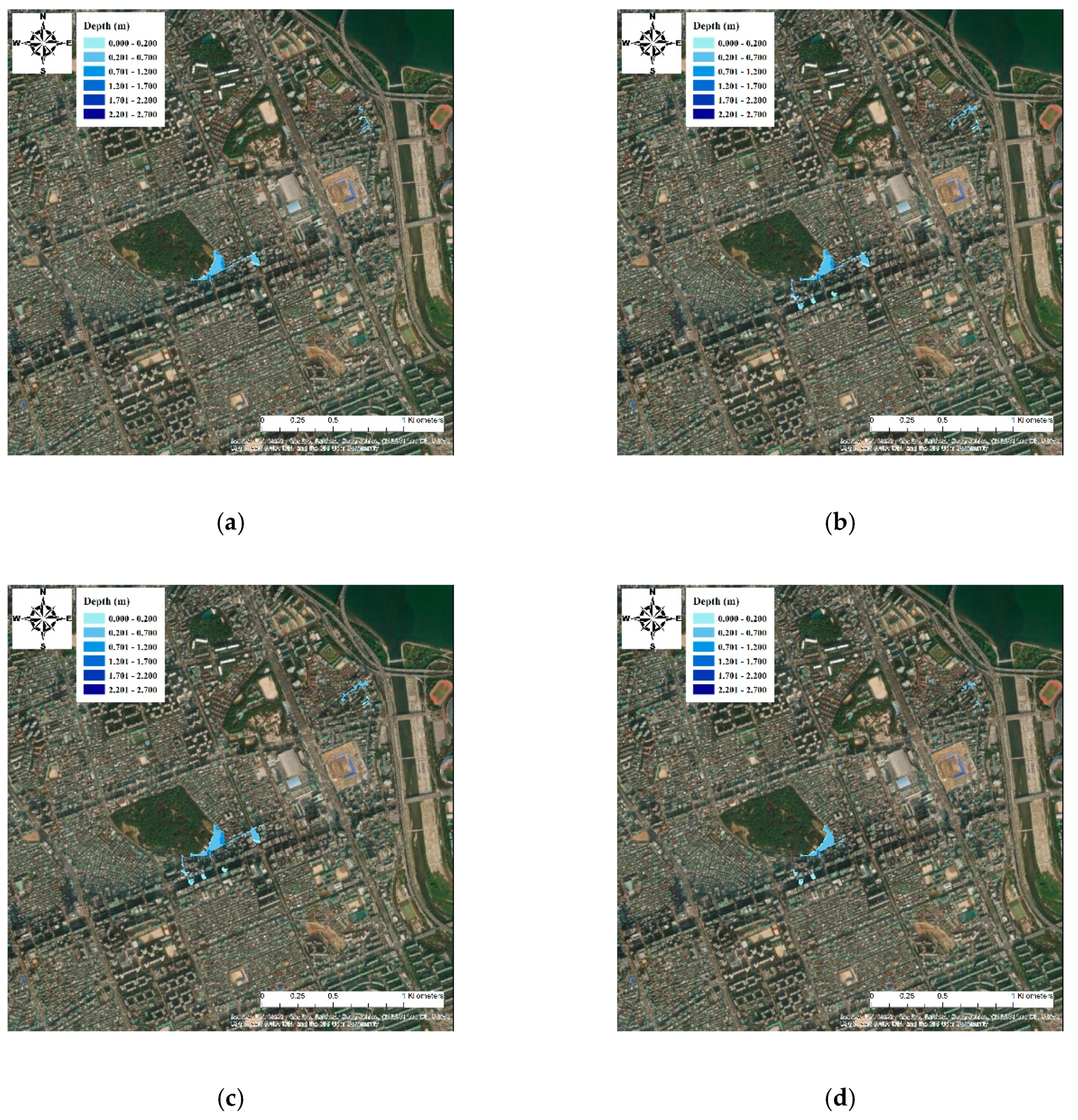
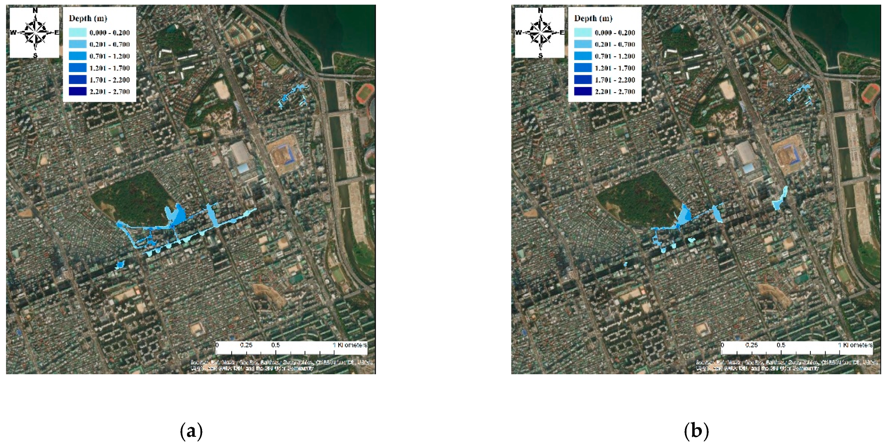
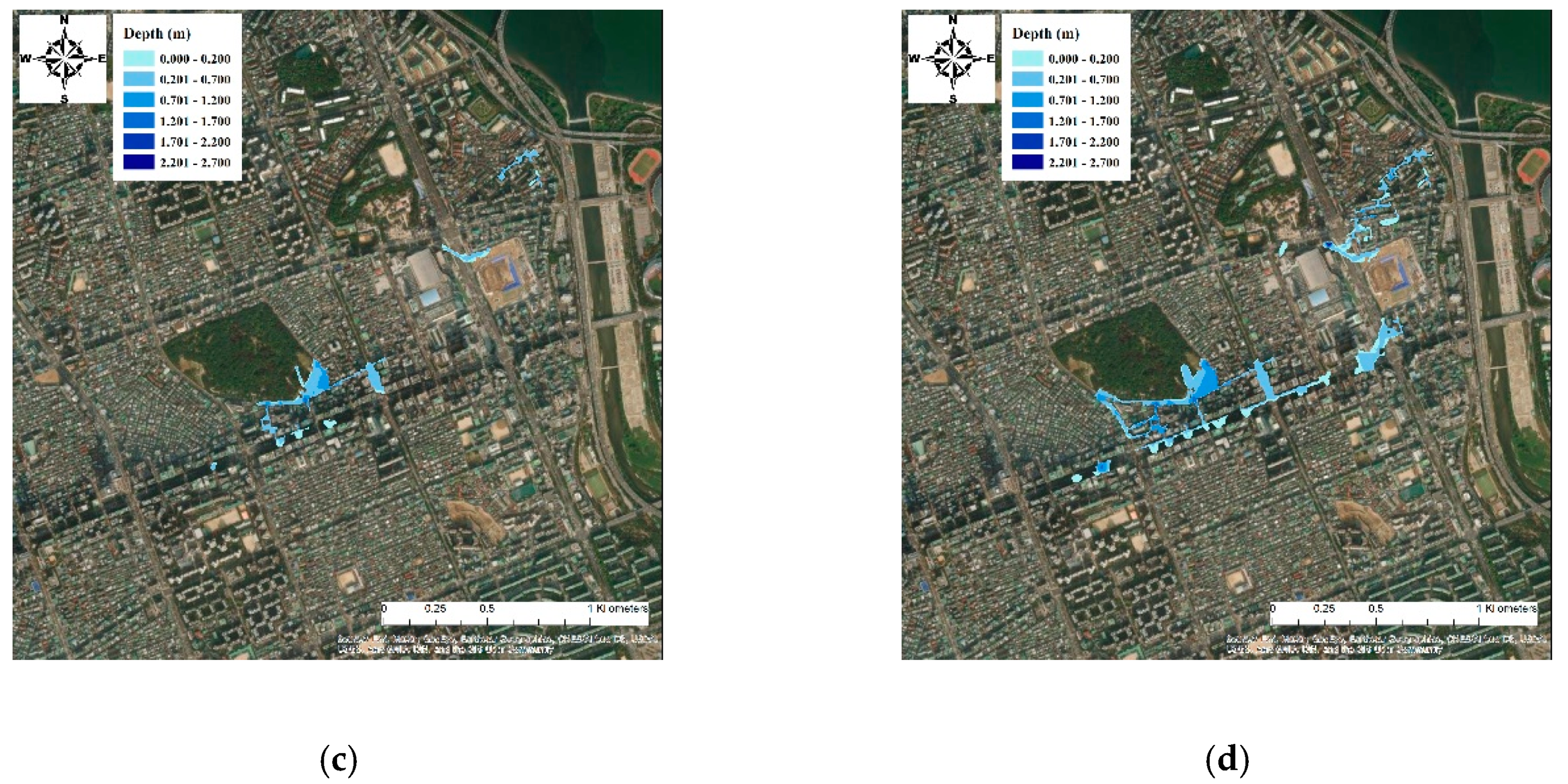
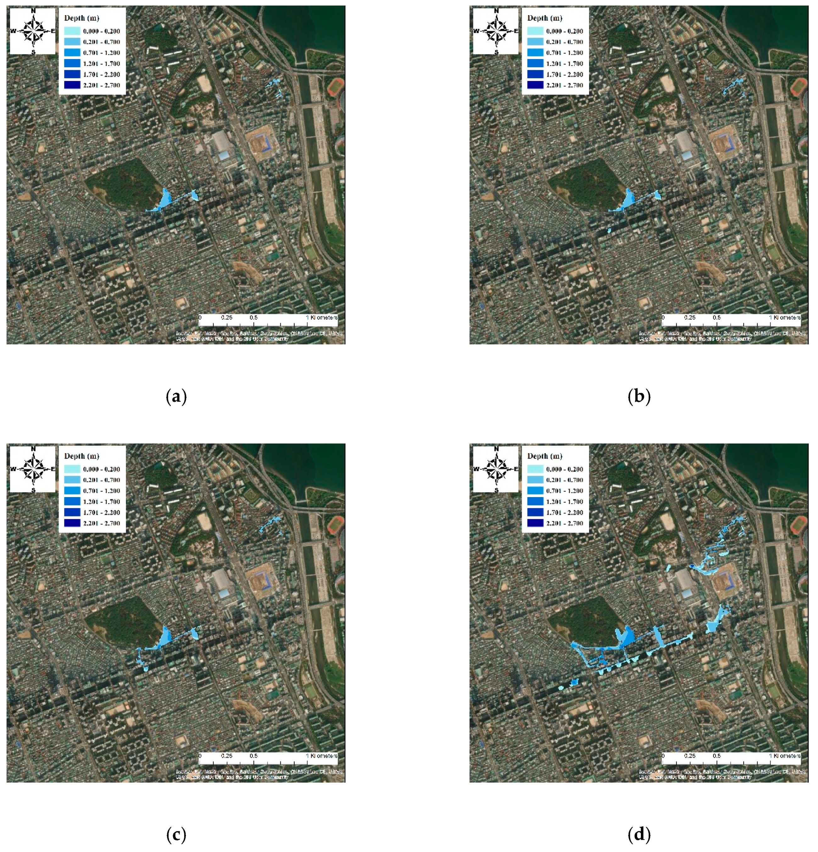
3.2. Perform of Optimum Inundation Map by FLO-2D Model

The overflow calculated by considering the simulated results for accumulated overflow from 342 manholes was used as the input data for the 2D hydraulic analysis program (FLO-2D model) based on the finite-difference method, as well as generated optimum inundation maps that can reflect maximum flood depth. According to the simulated total overflow results, most of the simulated maximum values of total overflow in the same year exist in different quartiles. Thus, the minimum and maximum flood occurrence maps were generated for different quantiles in the same year (Figure 7, Figure 8 and Figure 9), using the simulated results of a 1-h minimum, and maximum total overflow for the 100 years from the 1st to the 4th quartile of the Huff method. Figure 7 shows the minimum flood occurrence map results; over the 100 years, the largest flood scale can be seen in the map of the 3rd quartile. Similarly, Figure 8 shows that over 100 years, the largest flood scale can be found in the map of the 4th quartile. Figure 9 shows the simulated results of 100-year 1-h rainfall events with different exceedance probabilities (10%, 30%, 60%, 90%) of the Huff 4th quartile. The results showed that different exceedance probabilities for Huff events also produce different flood inundation responses. This means that the temporal concentration level of storms has a strong influence on the inundation behaviors, even when they occur in the same temporal peak location.
The results demonstrated that the same quantity of rainfall events showed considerable differences in overflow quantities with different time distribution characteristics. The difference between overflow amount and temporal distribution showed the different inundation behaviors. The rainfall event of the 4th quartile, with a 90% exceedance probability according to the Huff distribution, showed the maximum manhole overflow and widest range of inundation. The results showed that the temporal characteristics of storms, such as the temporal location of the storm peak and concentration level should be considered in order to generate the optimal inundation map to establish inundation prevention measures and conduct preliminary analysis and identification of the flood risk areas in urban drainage basins.

3.3. Discussion

Boxplots of the simulated total manhole overflow provide a visual summary of the results of 432 different rainfall scenarios reflecting the temporal characteristics of rainfall events such as the temporal concentration level and the temporal location of the storm peak. The rainfall scenarios consisted of nine different exceedance probabilities (10–90%), four different quartiles (1–4th quartile) of the Huff method, three different storm durations (1–3 h) and four different return periods (10, 50, 80, and 100-year) (Figure 10). The difference between the maximum and minimum total overflow with different temporal concentration levels of the 1, 2, and 3 h 10-year return period was 28.4 to 340.4 m3 (the maximum total overflow was 1.4 to 10.5 times larger than the minimum total overflow), the difference between maximum total overflow and minimum with different temporal concentration levels of the 1, 2 and 3 h 100-year return period was 101 to 1323.8 m3 (the maximum total overflow was 1.5 to 4.7 times the minimum total overflow), shown according to the growth in the return period and duration, has the larger difference in overflow quantity with the same rainfall amount, and is related to temporal concentration levels. In addition, the difference between maximum total overflow and minimum in the 1st quartile of the 1, 2, and 3 h 10 to 100-year return period was 87.4 to 928.8 m3 (the maximum total overflow was 2.8 to 10.5 times larger than the minimum total overflow), whereas the difference between maximum total overflow and minimum in the 2nd quartile of the 1, 2, and 3 h 10 to 100-year return period was 28.4 to 485.9 m3 (the maximum total overflow was 1.4 to 2.6 times larger than the minimum total overflow). Furthermore, the difference between maximum total overflow and minimum in the 3rd quartile of the 1, 2, and 3 h 10 to 100-year return period was 44 to 323.6 m3 (the maximum total overflow was 1.4 to 1.7 times larger than the minimum total overflow). The difference between maximum total overflow and minimum in the 4th quartile of the 1, 2, and 3 h 10 to 100-year return period was 89.8 to 1323.8 m3 (the maximum total overflow was 3.1 to 4.9 times larger than the minimum total overflow). The simulated total overflow results for the different quartiles in the same period showed that most of the simulated maximum values of total overflow in the same year exist in different quartiles. The simulated total overflow results also showed considerable differences.
Overall, the results demonstrated that the average total overflow increases with the increase in the quartile of the storm peak location. The maximum total overflow generally occurred when the storm peak was located in the 4th quartile. The minimum total overflow generally occurred when the storm peak was located in the 1st quartile. Nevertheless, the difference between the maximum and minimum total overflow in the 1st and 4th quartile was greater than that of the 2nd and 3rd quartile. The storm concentration level effect on the total overflow is larger than that of the storm peak location. This means that accurate time distribution characteristics of rainfall events are essential for a correct understanding and response to unban flood management. Even though the results showed that the total overflow is highly related to the storm concentration level and the temporal location of the storm peak, there are limitations to generalizing the results since the results are generated by a case study of an urban drainage basin. To overcome the locality issues and to enhance the applicability, extensive further research is necessary to generalize the relationships between the characteristics of time distribution of heavy storms and manhole overflow.

4. Conclusions

The urban flood inundation impacts associated with the temporal characteristics of heavy storms were analyzed for a target drainage basin in Seoul, Korea. The total manhole overflow and the inundation behavior were simulated using the EPA-SWMM and the FLO-2D model, respectively. Rainfall scenarios reflecting the temporal characteristics of rainfall events, such as the temporal concentration level and the temporal location of the storm peak were created using the Huff method for nine different exceedance probabilities (10–90%), for four different quartiles (1–4th quartile), for three different storm durations (1–3 h) and four different return periods (10, 50, 80, and 100-years).
The simulated manhole overflow and inundation area were highly related to the temporal characteristics of storms, not only the temporal location of the storm peak but also the concentration level. The manhole overflow with different temporal concentration levels of 1, 2, and 3 h 10-year return period events showed a 4.8, 7.2 and 10.5 times difference, respectively. This means that the longer rainfall duration has the larger difference in overflow quantity with the same rainfall amount. The overflow amount with different temporal concentration levels of 1, 2, and 3 h 100-year return period events showed a 3.7, 3.8 and 2.8 times difference, respectively.
The manhole overflow with different temporal locations of the storm peak of 1, 2, and 3 h 10-year return period events showed a 29.7, 98.5 and 79.1%, difference, respectively. The manhole overflow with different temporal locations of the storm peak of 1, 2, and 3 h 100-year return period events showed a 2.17, 1.92 and 1.65 times difference, respectively. The rainfall event in the 4th quartile, with 90% exceedance in terms of Huff distribution probability, showed the maximum manhole overflow and widest inundation range. The results also illustrated that the temporal concentration level is more effective in determining the manhole overflow amount than the temporal location of the storm peak.
The results illustrate that despite the same rainfall quantity, there is a huge difference in the manhole overflow amount and the inundation area according to the difference in the time distribution characteristics. Therefore, a consideration of the temporal distribution characteristics of extreme rainfall events is essential for an accurate understanding of the rainfallrunoff response and the inundation behavior in urban areas. The results also show the possibility of establishing appropriate inundation prevention measures in urban drainage basins when rainfall forecasts including not only quantity but also time distribution characteristics are available.

Author Contributions

T.L., G.L. and G.K. conceived and designed the experiments; T.L. performed the experiments; G.K. provided the Huff rainfall data; T.L. ran the EPA-SWMM and FLO-2D model; T.L. analyzed the data; G.K. and G.L. supervision experiments; T.L. wrote the paper. All authors have read and agreed to the published version of the manuscript.

Funding

This research was funded by the Korea Environmental Industry & Technology Institute (KEITI) of the Korea Ministry of Environment (MOE) as part of the “Advanced Water Management Research Program”. (79615).

Institutional Review Board Statement

Not applicable.

Informed Consent Statement

Not applicable.

Data Availability Statement

Authors have the raw data readily available for presentation to the referees and the editors of the journal, if requested. Authors ensure appropriate analysis are taken so that raw data is retained in full for a reasonable time after publication.

Acknowledgments

This work was supported by the Korea Environmental Industry & Technology Institute (KEITI) of the Korea Ministry of Environment (MOE) as part of the “Advanced Water Management Research Program”. (79615).

Conflicts of Interest

The authors declare no conflict of interest.

References

  1. Westra, S.; Fowler, H.J.; Evans, J.P.; Alexander, L.V.; Berg, P.; Johnson, F.; Kendon, E.J.; Lenderink, G.; Roberts, N.M. Future changes to the intensity and frequency of short-duration extreme rainfall. Rev. Geophys. 2014, 52, 522–555. [Google Scholar] [CrossRef]
  2. Jha, A.K.; Bloch, R.; Lamond, J. Cities and Flooding: A Guide to Integrated Urban Flood Risk Management for the 21st Century; The World Bank: Washington, DC, USA, 2012; pp. 1–631. [Google Scholar]
  3. Wang, X.; Kinsland, G.; Poudel, D.; Fenech, A. Urban flood prediction under heavy precipitation. J. Hydrol. 2019, 577, 1–21. [Google Scholar] [CrossRef]
  4. Myronidis, D.; Stathis, D.; Sapountzis, M. Post-Evaluation of flood hazards induced by former artificial interventions along a coastal Mediterranean settlement. J. Hydrol. Eng. 2016, 21, 05016022. [Google Scholar] [CrossRef]
  5. Korea Meteorological Administration (KMA). Climate Change Projection Report on Korean Peninsula, Seoul, Republic of Korea; Korea Meteorological Administration: Seoul, Korea, 2012; pp. 1–40.
  6. Gantidis, N.; Pervolarakis, M.; Fytianos, K. Assessment of the quality characteristics of two Lakes (Koronia and Volvi) of N. Greece. Environ. Monito. Assess. 2007, 125, 175–181. [Google Scholar] [CrossRef] [PubMed]
  7. Hwang, K.; Schuetze, T.; Amoruso, F.M. Flood Resilient and Sustainable Urban Regeneration Using the Example of an Industrial Compound Conversion in Seoul, South Korea. Sustainability 2020, 12, 918. [Google Scholar] [CrossRef] [Green Version]
  8. Kim, J.; Kuwahara, Y.; Kumar, M. A DEM-based evaluation of potential flood risk to enhance decision support system for safe evacuation. Nat. Hazards 2011, 59, 1561–1572. [Google Scholar] [CrossRef]
  9. Keifer, G.J.; Chu, H.H. Synthetic storm pattern for drainage design. J. Hydraul. Div. 1957, 83, 1–25. [Google Scholar] [CrossRef]
  10. Yen, B.C.; Chow, V.T. Design hyetographs for small drainage structures. J. Hydraul. Div. 1980, 106, 1055–1076. [Google Scholar] [CrossRef]
  11. Soil Conservation Service (SCS). Urban hydrology for small watersheds. In Technical Release 55; U.S. Department of Agriculture: Washington, DC, USA; Soil Conservation Service: Washington, DC, USA, 1986. [Google Scholar]
  12. Huff, F.A. Time distributions of heavy rainstorms in Illinois. In Illinois State Water Survey, Circular 173; Illinois State Water Survey: Champaign, IL, USA, 1990. [Google Scholar]
  13. Myronidis, D.; Ioannou, K. Forecasting the urban expansion effects on the design storm hydrograph and sediment yield using artificial neural networks. Water 2019, 11, 31. [Google Scholar] [CrossRef] [Green Version]
  14. Choi, S.Y.; Joo, K.W.; Shin, H.J.; Heo, J.H. Improvement of Huff’s Method Considering Severe Rainstorm Events. J. Korea Water Resour. Assoc. 2014, 47, 985–996. [Google Scholar] [CrossRef]
  15. Yang, Y.; Sun, L.; Li, R.; Yin, J.; Yu, D. Linking a storm water management model to a novel two-dimensional model for urban pluvial flood modeling. Int. J. Disaster Risk Sci. 2020, 11, 508–518. [Google Scholar] [CrossRef]
  16. Bezak, N.; Šraj, M.; Rusjan, S.; Mikoš, M. Impact of the rainfall duration and temporal rainfall distribution defined using the Huff curves on the hydraulic flood modelling results. J. Geosci. 2018, 8, 69. [Google Scholar] [CrossRef] [Green Version]
  17. Lee, B.J. Analysis on inundation characteristics for flood impact forecasting in Gangnam drainage basin. J. Atmo. 2017, 27, 189–197. [Google Scholar]
  18. Erena, S.H.; Worku, H.; Paola, F.D. Flood hazard mapping using FLO-2D and local management strategies of Dire Dawa city, Ethiopia. J. Hydrol. Reg. Stud. 2018, 19, 224–239. [Google Scholar] [CrossRef]
  19. Luo, P.; Mu, D.; Xue, H.; Duc, T.N.; Dinh, K.D.; Takara, K.; Nover, D.; Schladow, G. Flood inundation assessment for the Hanoi Central Area, Vietnam under historical and extreme rainfall conditions. Sci. Rep. 2018, 12623. [Google Scholar] [CrossRef]
  20. Vojtek, M.; Petroselli, A.; Vojteková, J.; Asgharinia, S. Flood inundation mapping in small and ungauged basins: Sensitivity analysis using the EBA4SUB and HEC-RAS modeling approach. Hydrol. Resear. 2019, 50, 1002–1019. [Google Scholar] [CrossRef] [Green Version]
  21. GebreEgziabher, M.; Demissie, Y. Modeling Urban Flood Inundation and Recession Impacted by Manholes. Water 2020, 12, 1160. [Google Scholar] [CrossRef] [Green Version]
  22. Choi, S.; Yoon, S.; Lee, B.; Choi, Y. Evaluation of High-Resolution QPE data for Urban Runoff Analysis. J. Korea Water Resour. Assoc. 2015, 48, 719–728. [Google Scholar] [CrossRef] [Green Version]
  23. Ellouze, M.; Habib, A.; Riadh, S. A triangular model for the generation of synthetic hyetographs. Hydrol. Sci. J. 2009, 54, 287–299. [Google Scholar] [CrossRef]
  24. Kang, M.S.; Goo, J.H.; Song, I.; Chun, J.A.; Her, Y.G.; Hwang, S.W.; Park, S.W. Estimating design floods based on the critical storm duration for small watersheds. J. Hydro-Environ. Res. 2013, 7, 209–218. [Google Scholar] [CrossRef]
  25. Yoon, S.S.; Bae, D.H.; Choi, Y.J. Urban Inundation Forecasting Using Predicted Radar Rainfall: Case Study. J. Korean Soc. Hazard. Mitig. 2014, 14, 117–126. [Google Scholar] [CrossRef] [Green Version]
  26. Shin, S.Y.; Yeo, C.G.; Baek, C.H.; Kim, Y.J. Mapping Inundation Areas by Flash Flood and Developing Rainfall Standards for Evacuation in Urban Settings. J. Korean Assoc. Geogr. Inf. Stud. 2005, 8, 71–80. [Google Scholar]
  27. Huber, W.C.; Dickson, R.E. Storm Water Management Model. User’s Manual Version 4; Environmental Protection Agency: Washington, DC, USA, 1988.
  28. Park, J.H.; Kim, S.H.; Bae, D.H. Evaluating Appropriateness of the Design Methodology for Urban Sewer System. J. Korea Water Resour. Assoc. 2019, 52, 411–420. [Google Scholar]
  29. Pellicani, R.; Parisi, A.; Iemmolo, G.; Apollonio, C. Economic risk evaluation in urban flooding and instability-prone areas: The case study of San Giovanni Rotondo (Southern Italy). Geosciences 2018, 8, 112. [Google Scholar] [CrossRef] [Green Version]
  30. Risi, R.D.; Jalayer, F.; Paola, F.D. Meso-scale hazard zoning of potentially flood prone areas. J. Hydrol. 2015, 527, 316–325. [Google Scholar] [CrossRef]
  31. Hromadka, T.V.; Guymon, G.L.; Pardoen, G.C. Nodal domain integration model of unsaturated two-dimensional soil-water flow: Development. Water Resour. Res. 1981, 17, 1425–1430. [Google Scholar] [CrossRef]
  32. Kim, H.I.; Han, K.Y. Inundation Map Prediction with Rainfall Return Period and Machine Learning. Water 2020, 12, 1552. [Google Scholar] [CrossRef]
Figure 1. Location of the study area in the Samsung-dong and flood risk zone.
Water 13 03438 g001
Figure 2. (a) Actual rainfall sample on 21 September 2010 and (b) 6-h extreme Huff rainfall sample.
Water 13 03438 g002aWater 13 03438 g002b
Figure 3. Verification of two-dimensional flood analysis results.
Water 13 03438 g003
Figure 4. Flowchart of study methodology.
Water 13 03438 g004
Figure 5. Digital elevation model (DEM) for the target area.
Water 13 03438 g005
Figure 6. The exact location of each manhole was adjusted by the ArcGIS model.
Water 13 03438 g006
Figure 7. Sample minimum inundation maps applying 100-year, 1-h rainfall events with different Huff quartile distributions ((ad): 1st, 2nd, 3rd, and 4th quartile).
Water 13 03438 g007
Figure 8. Sample maximum inundation maps applying 100-year, 1-h rainfall events with different Huff quartile distributions ((ad): 1st, 2nd, 3rd, and 4th quartile).
Water 13 03438 g008aWater 13 03438 g008b
Figure 9. Sample inundation maps applying 100-year, 1-h rainfall events with different exceedance probabilities ((a–d): 10%, 30%, 60%, 90%) of Huff 4th quartile distribution.
Water 13 03438 g009
Figure 10. Boxplots of the EPA-SWMM-model-simulated total overflow from 1 to 3 h for a period from 10 to 100 years ((a) total overflow of 1-h rainfall, (b) total overflow of 2-h rainfall, (c) total overflow of 3-h rainfall).
Water 13 03438 g010aWater 13 03438 g010b
Table 1. 1, 2, and 3-h total rainfall during different return periods.
Duration (Hour)Total Rainfall by Periods (mm)
10 Years50 Years80 Years100 Years
172.691.596.699.01
2108.6140.4149.2153.3
3136.2181.4194.5200.6
Table 2. The EPA-SWMM-model-simulated 1-h total overflow results.
Huff
Quartile
Period
(Year)
Total Overflow According to Different Exceedance Probabilities (m3)Average
(m3)
Minimum
(m3)
Maximum
(m3)
10%20%30%40%50%60%70%80%90%
1st10 110.270.274.472.767.158.946.432.022.861.622.8110.2
50 395.0206.3133.3118.8122.8129.7118.3117.5114.3161.8114.3395.0
80 489.7222.6167.8137.0149.3142.4141.4136.8132.4191.0132.4489.7
100 536.0263.9180.1149.8153.9153.1149.3146.6156.8209.9146.6536.0
2nd10 102.798.9101.3101.084.085.182.077.974.389.774.3102.7
50 189.9187.9158.0156.8157.9140.1148.6201.0156.1166.3140.1201.0
80 236.4233.5182.5173.6173.0160.0169.4172.3183.7187.2160.0236.4
100 290.4225.9192.8236.2186.4186.0179.5184.0201.2209.2179.5290.4
3rd10 71.484.089.485.993.695.893.0108.0115.492.971.4115.4
50 159.6168.6165.8162.7159.5170.7176.8200.7205.8174.5159.5205.8
80 190.2192.5185.2184.8185.0202.8215.2217.3268.1204.6184.8268.1
100207.5197.4196.5195.7206.7217.3232.0241.8296.7221.3195.7296.7
4th10 43.454.265.577.588.393.897.1111.0133.284.943.4133.2
50 113.7122.2119.7132.2134.2153.5179.1263.5486.8189.4113.7486.8
80 139.2149.1153.1154.8167.7189.7241.1371.7639.1245.1139.2639.1
100153.0152.2156.8166.0184.1203.0368.3447.4718.2283.2152.2718.2
Table 3. The EPA-SWMM-model-simulated duration 2-h total overflow results.
Huff
Quartile
Period
(Year)
Total Overflow According to Different Exceedance Probabilities (m3)Average
(m3)
Minimum
(m3)
Maximum
(m3)
10%20%30%40%50%60%70%80%90%
1st10 203.5166.1142.6110.293.868.955.441.528.1101.128.1203.5
50 673.9370.4331.8287.8256.5221.0185.2216.0156.2299.9156.2673.9
80 921.6489.6403.7386.8351.8322.7288.1232.9237.0403.8232.9921.6
100 1050.6549.6446.0426.9390.0374.8346.6303.6275.5462.6275.51050.6
2nd10 182.1175.5146.9161.2157.1129.3117.8113.693.8141.993.8182.1
50 478.2400.1378.1379.0355.4346.9324.3323.4352.0370.8323.4478.2
80 656.0520.9463.3461.0466.4432.5419.4421.0442.4475.9419.4656.0
100 739.1574.3510.0509.9504.1472.7462.1460.2488.2524.5460.2739.1
3rd10 128.2121.2150.8156.8153.7163.3177.9182.0201.9159.5121.2201.9
50 374.1371.3384.2402.2490.6436.3451.8463.9528.1433.6371.3528.1
80 507.2475.6482.6499.1531.9630.2556.0596.3652.7548.0475.6652.7
100588.9523.8541.6546.5574.8569.9613.6659.3727.3594.0523.8727.3
4th10 74.399.4121.0148.2165.6178.7212.2231.7361.5177.074.3361.5
50 255.9347.8326.3403.9418.6462.8590.5661.9985.7494.8255.9985.7
80 346.4383.8427.5507.1537.9601.4785.2874.41266.9636.7346.41266.9
100394.1435.7473.8561.5584.7687.7888.1988.01394.2712.0394.11394.2
Table 4. The EPA-SWMM-model-simulated total overflow results for a 3-h duration.
Huff
Quartile
PeriodTotal Overflow According to Different Exceedance Probabilities (m3)Average
(m3)
Minimum
(m3)
Maximum
(m3)
10%20%30%40%50%60%70%80%90%
1st10 286.5216.6176.9122.5105.584.956.334.827.3123.527.3286.5
50 917.3601.9523.1480.7439.2395.5333.9298.3311.0477.9298.3917.3
80 1271.4746.8682.7611.1575.8532.4496.7463.5450.9647.9450.91271.4
100 1448.1847.9740.9693.1652.0603.8563.9557.1519.3736.2519.31448.1
2nd10 256.8250.3183.4122.5178.5155.4132.4121.3100.0166.7100.0256.8
50 800.9634.8605.9584.2582.8566.2532.4528.2534.4596.6528.2800.9
80 1091.2900.6764.5755.4735.5729.3690.0661.7712.9782.3661.71091.2
100 1232.9916.5839.6838.3816.1800.2761.0747.0783.3859.4747.01232.9
3rd10 174.1192.3194.9210.9220.6227.6236.1256.5371.3231.6174.1371.3
50 600.4619.7625.9650.6698.7700.0717.9810.5828.7694.7600.4828.7
80 810.4808.8811.6834.0885.8903.8913.9947.21082.0888.6808.81082.0
100940.2907.3902.5911.7988.2998.81030.11062.51226.1996.4902.51226.1
4th10 119.5136.5179.7234.7243.4271.6339.3439.5459.9269.3119.5459.9
50 469.2503.9563.1691.5729.0876.6966.9984.11456.6804.5469.21456.6
80 633.3671.3725.5900.7944.81048.31272.51310.31847.91039.4633.31847.9
100703.4752.1815.71013.71068.91175.01423.71484.22027.21162.7703.42027.2
Publisher’s Note: MDPI stays neutral with regard to jurisdictional claims in published maps and institutional affiliations.

