
Flood Hazard Mapping with Distributed Hydrological Simulations and Remote-Sensed Slackwater Sediments in Ungauged Basins

 , , and
Abstract
:1. Introduction
2. Materials and Methods
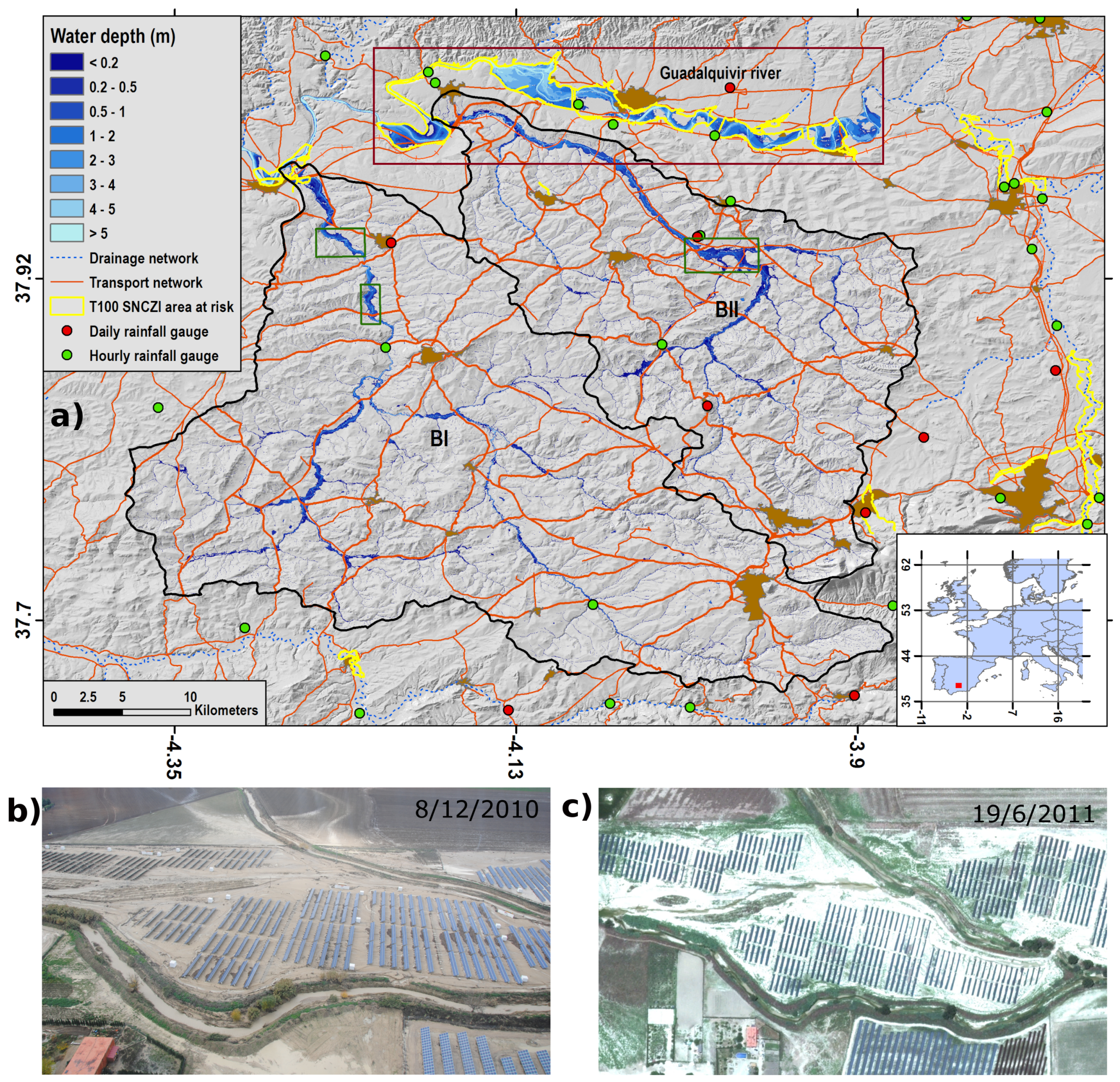
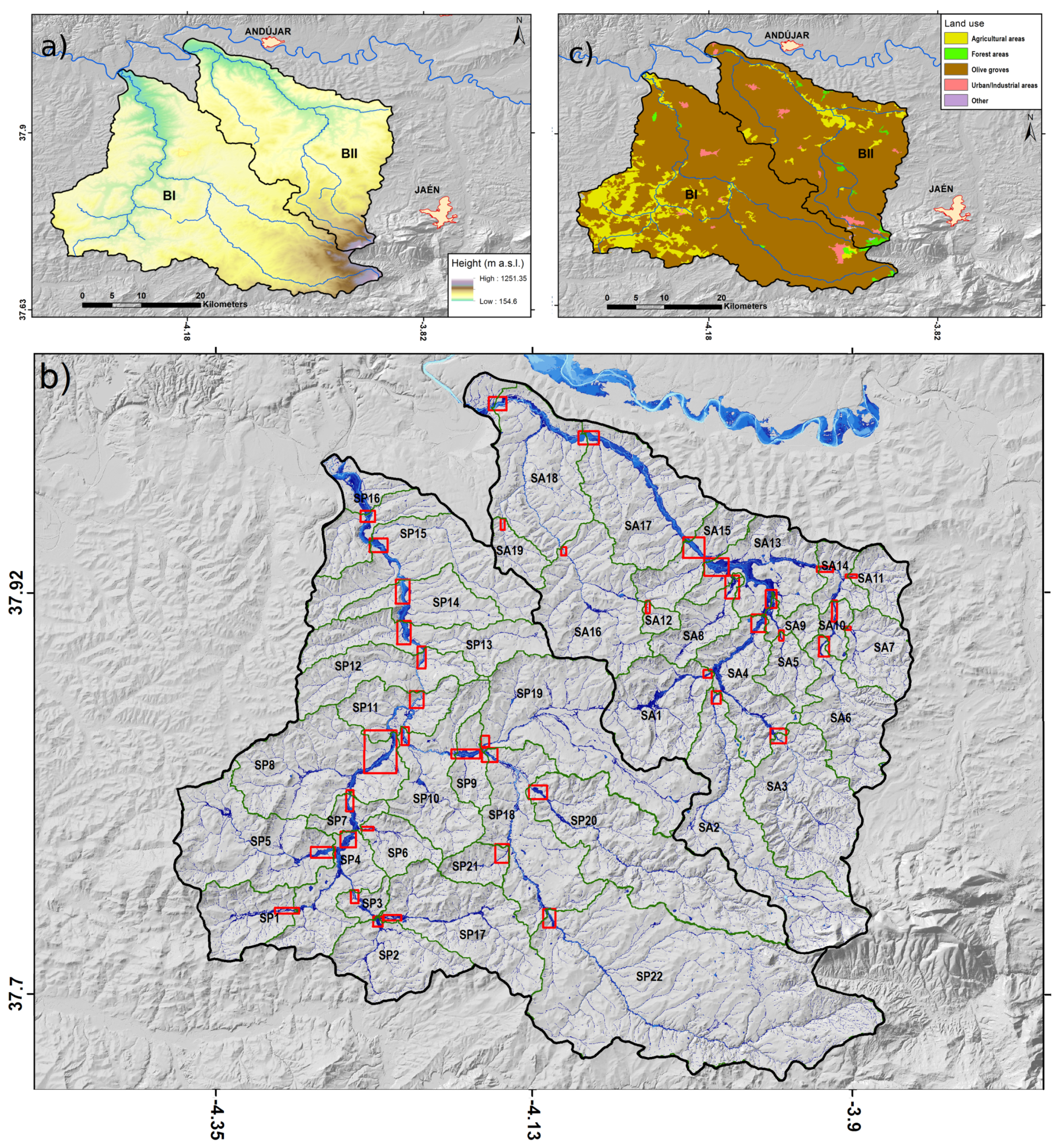
2.1. Study Site
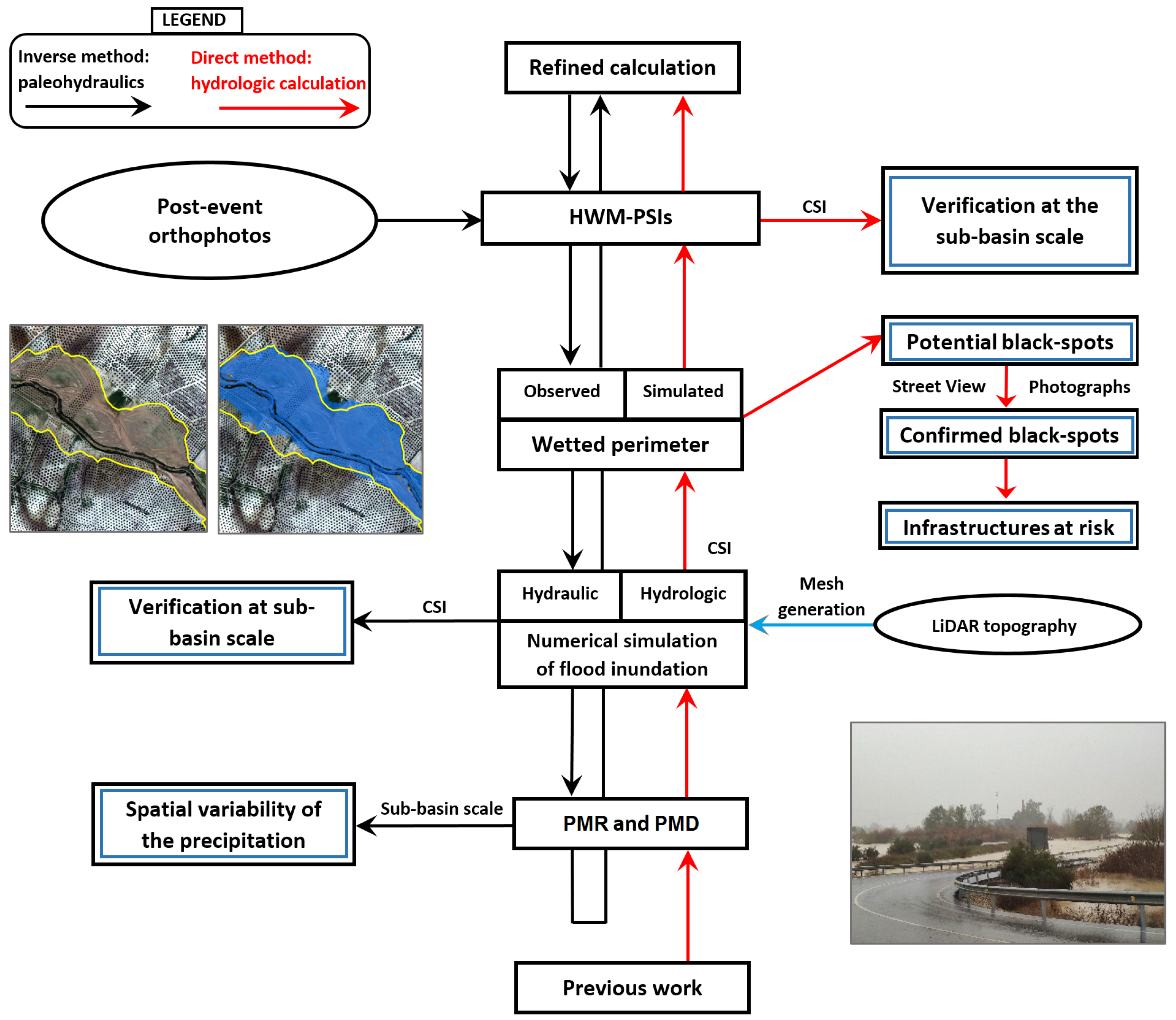
2.2. Methodology
2.2.1. Direct Method: Hydrological Calculation with Uniform Precipitation
2.2.2. Recursive Paleohydrological Reconstruction in Multiple Sub-Basins
2.2.3. Verification of the Simulated Water Level and Rainfall Databases
3. Results and Discussion
3.1. Quality of the Hydrological Calculation with a Uniform Precipitation
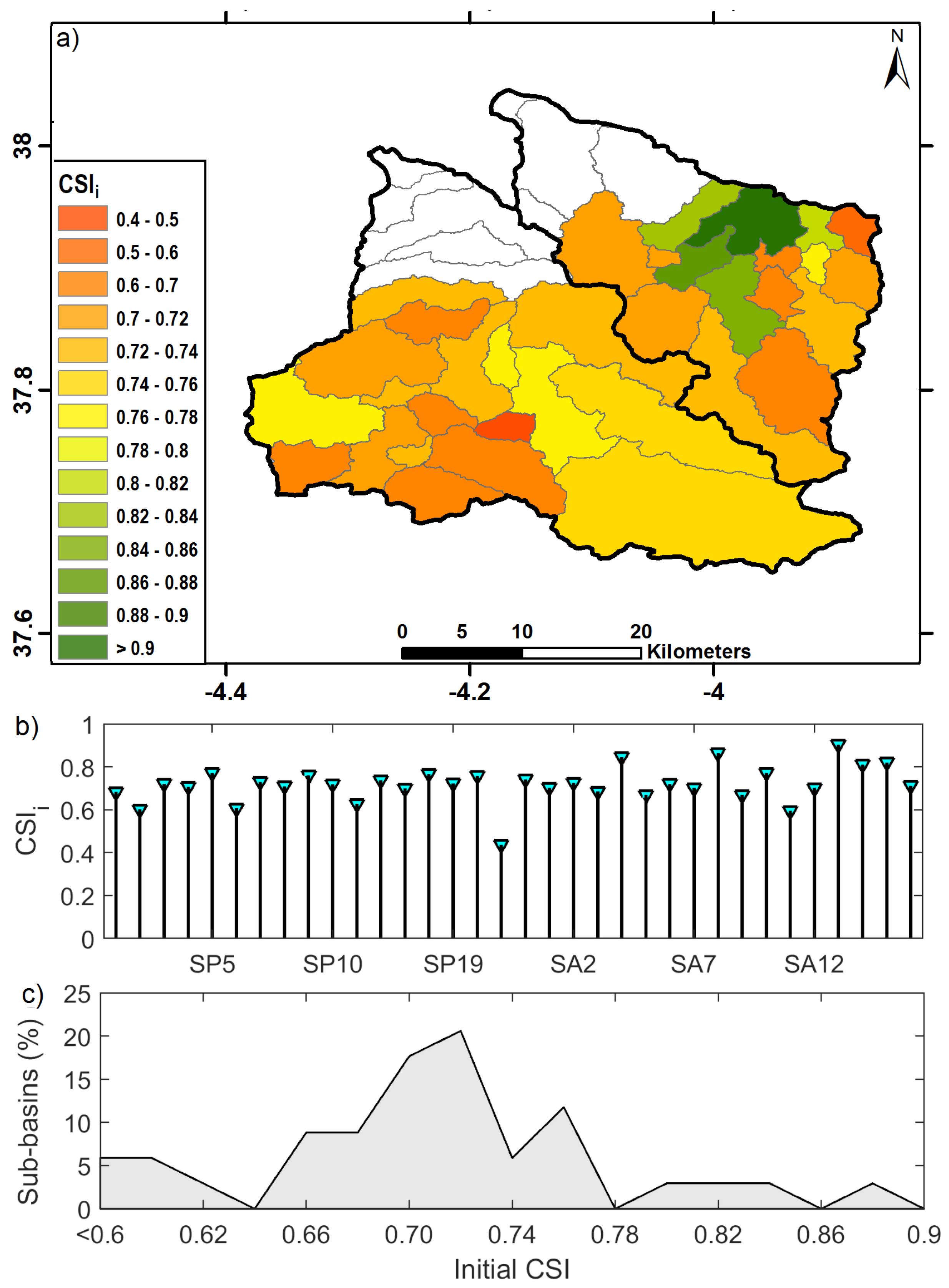
3.1.1. Verification of Flooding Maps through the Critical Success Index
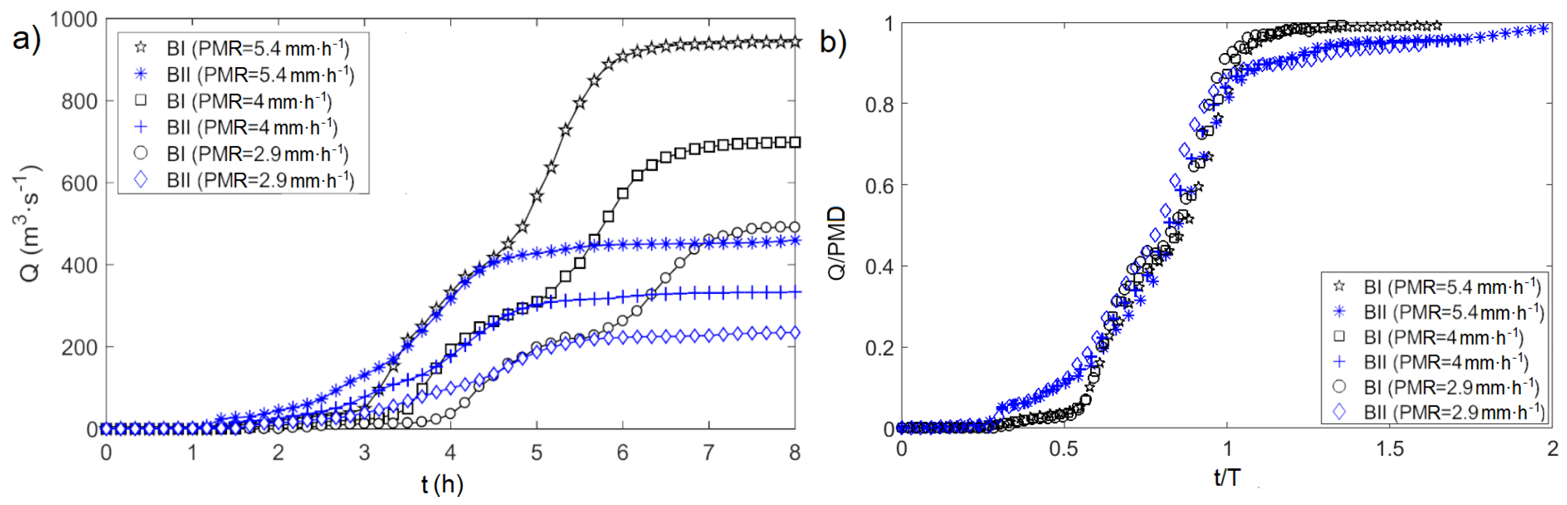
3.1.2. Dimensional and SELF-Similar Analysis of the Hydrograph: S-Curve
3.2. Recursive Paleohydrological Reconstruction at the Sub-Basin Scale
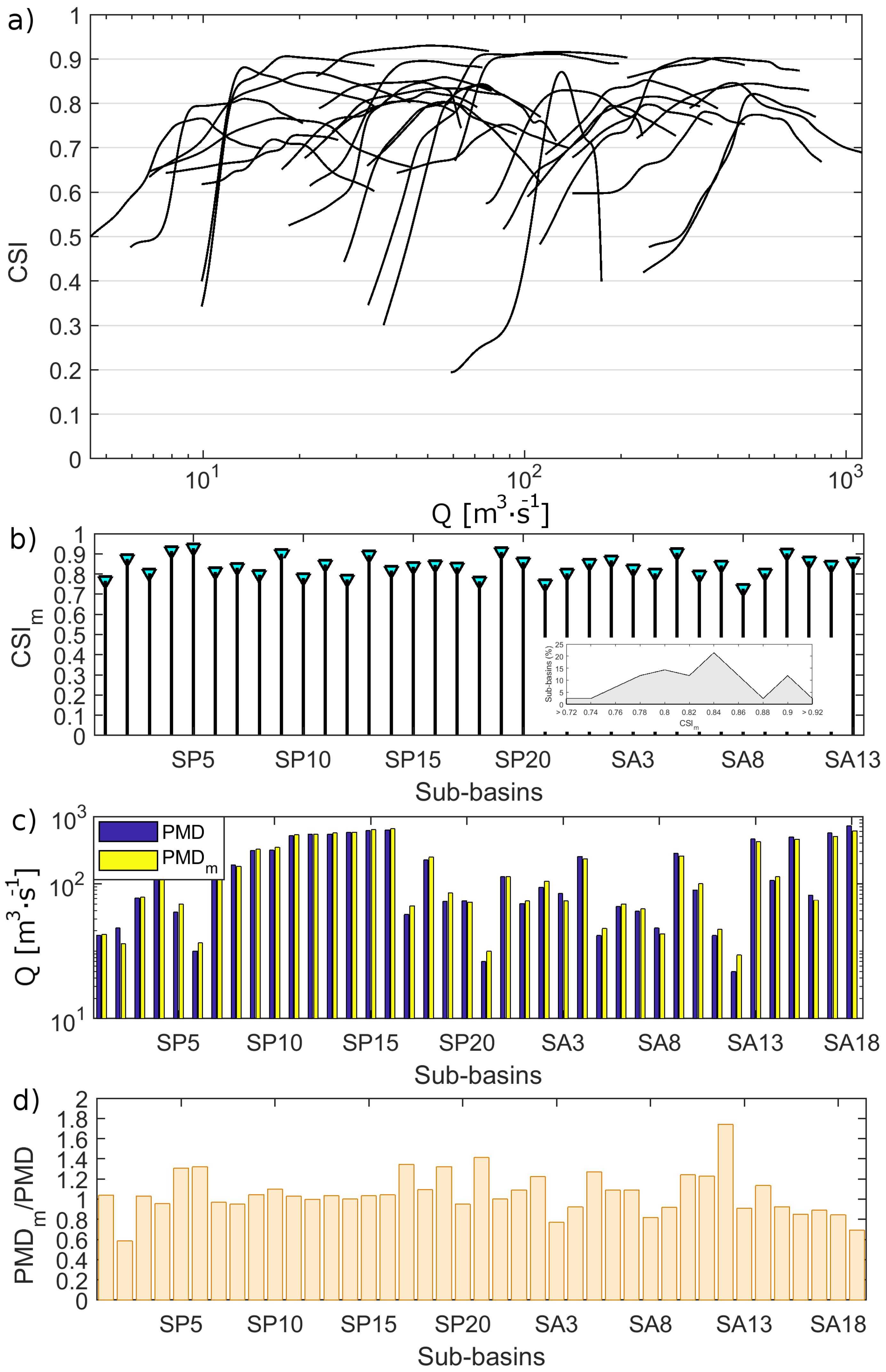
3.2.1. Peak Discharge Calculation from Optimal Analysis of CSI
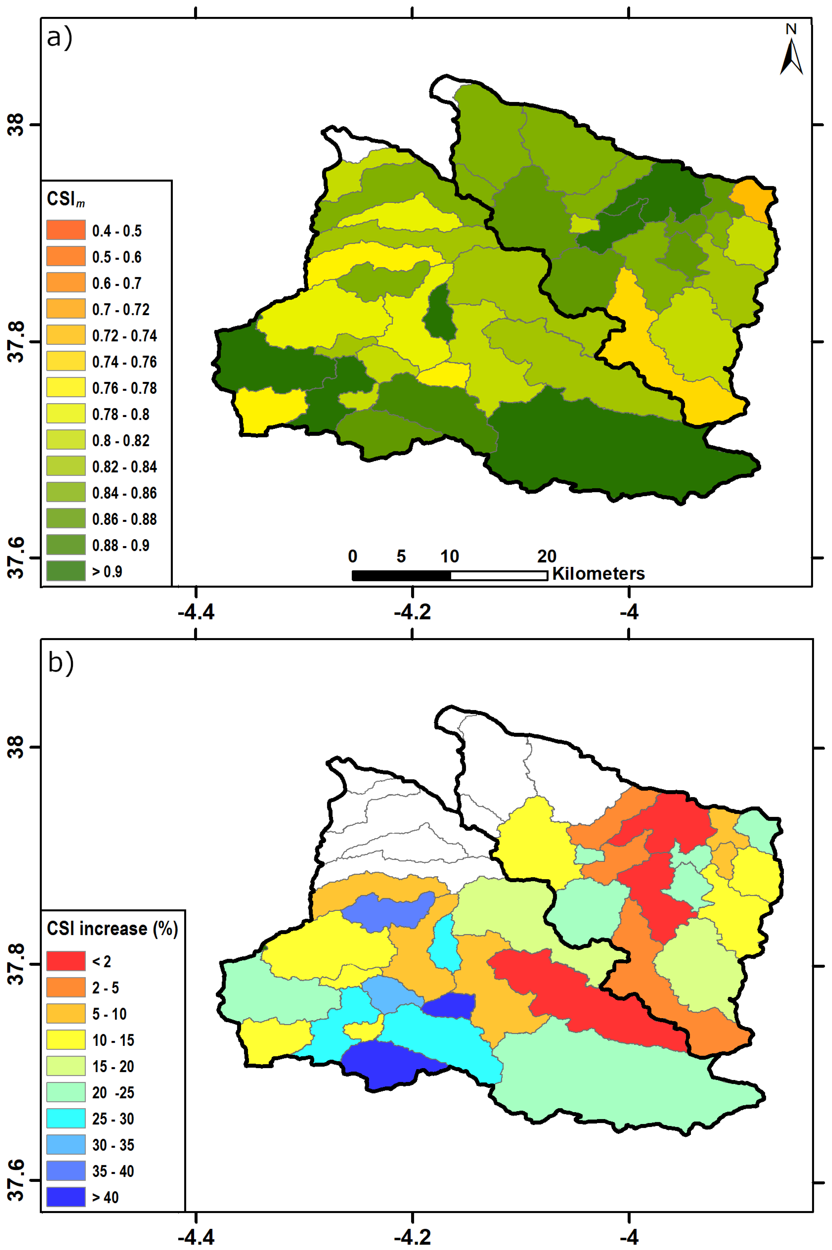
3.2.2. Spatial Distribution of the Precipitation
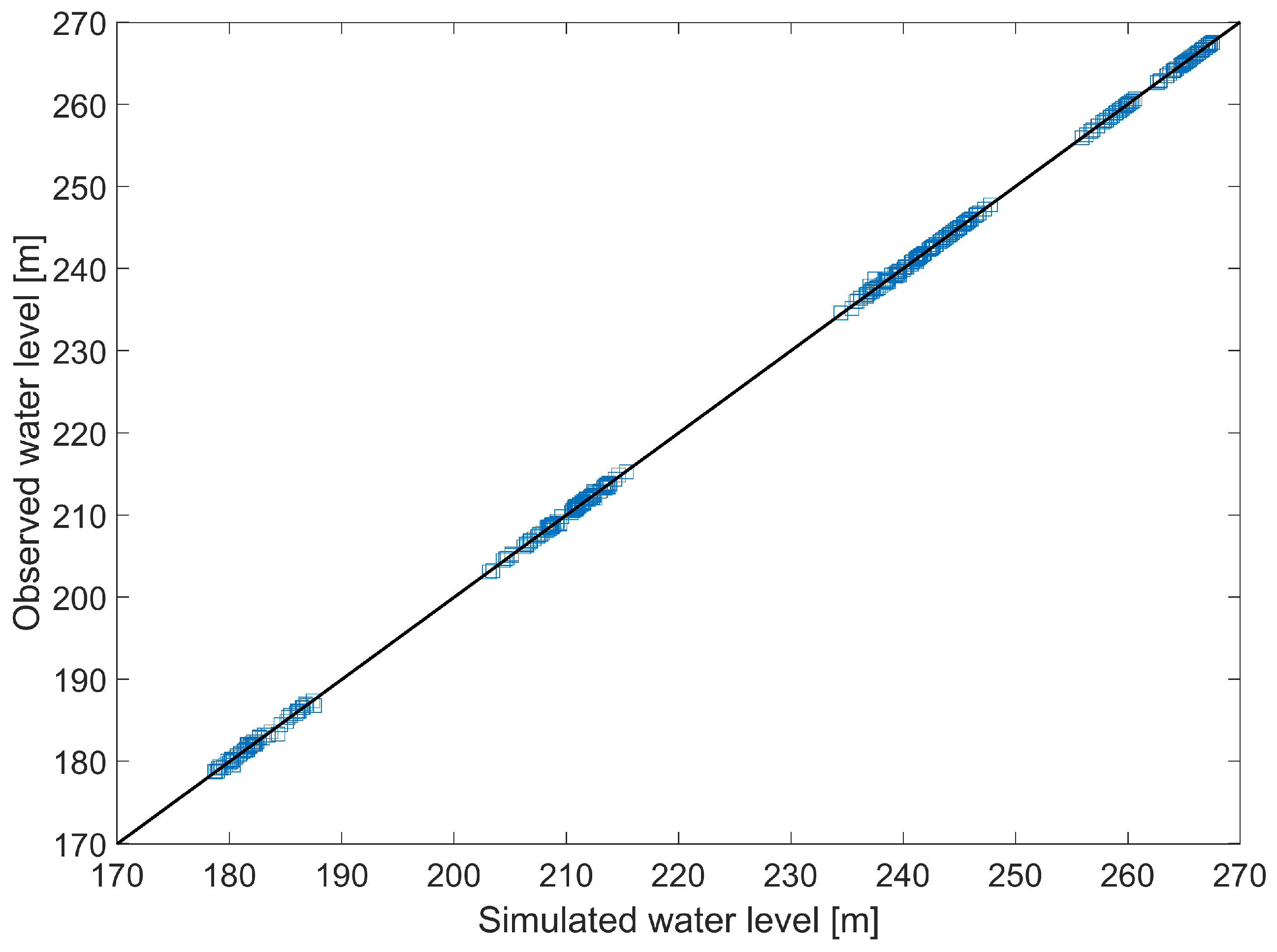
3.3. Verification of the Simulated Water Level and Rainfall Databases
4. Conclusions
Author Contributions
Funding
Institutional Review Board Statement
Informed Consent Statement
Data Availability Statement
Conflicts of Interest
Abbreviations
| BI | Basin I (Salado de Porcuna) |
| BII | Basin II (Salado de Arjona) |
| CPU | Central Processing Unit |
| CSI | Critical Success Index |
| DEM | Digital Elevation Model |
| GPU | Graphics Processing Unit |
| GPS | Global Positioning System |
| HWM | High-Water Marks |
| LiDAR | Light Detection and Ranging |
| PMD | Probable Maximum Discharge |
| PMR | Probable Maximum Rainfall |
| PSI | Paleo-Stage Indicator |
| IA | Index of Agreement |
| RMSE | Root Mean Square Error |
| MAPE | Mean Absolute Percentage of Error |
| BIAS | Bias Index |
| SI | Scatter Index |
References
- Moral-Erencia, J.; Bohorquez, P.; Jimenez-Ruiz, P.; Pérez-Latorre, F. Slackwater Sediments Record the Increase in Sub-daily Rain Flood due to Climate Change in a European Mediterranean Catchment. Water Resour. Manag. 2020, 34, 4431–4447. [Google Scholar] [CrossRef]
- IPCC. Climate Change 2013: The Physical Science Basis. Contribution of Working Group I to the Fifth Assessment Report of the Intergovernmental Panel on Climate Change; Stocker, T.F., Qin, D., Plattner, G.K., Tignor, M.M.B., Allen, S.K., Boschung, J., Nauels, A., Xia, Y., Bex, V., Midgley, P.M., Eds.; Cambridge University Press: Cambridge, UK, 2013; ISBN 978-92-9169-138-8. [Google Scholar]
- EEA. Climate Change, Impacts and Vulnerability in Europe 2016: An Indicator-Based Report; Publications Office of the European Union: Luxembourg, 2017; Number 1/2017. [Google Scholar] [CrossRef]
- Merz, R.; Blöschl, G. A process typology of regional floods. Water Resour. Res. 2003, 39, SWC510–SWC520. [Google Scholar] [CrossRef]
- Alfieri, L.; Thielen, J. A European precipitation index for extreme rain-storm and flash flood early warning. Meteorol. Appl. 2015, 22, 3–13. [Google Scholar] [CrossRef] [Green Version]
- Burguet, M.; Taguas, E.V.; Cerdà, A.; Gómez, J. Soil water repellency assessment in olive groves in Southern and Eastern Spain. Catena 2016, 147, 187–195. [Google Scholar] [CrossRef]
- Merz, B.; Thieken, A.; Gocht, M. Flood Risk Mapping At The Local Scale: Concepts and Challenges. In Flood Risk Management in Europe: Innovation in Policy and Practice; Begum, S., Stive, M.J.F., Hall, J.W., Eds.; Springer: Dordrecht, The Netherlands, 2007; pp. 231–251. [Google Scholar] [CrossRef]
- Nones, M.; Caviedes-Voullième, D. Computational advances and innovations in flood risk mapping. J. Flood Risk Manag. 2020, 13, e12666. [Google Scholar] [CrossRef]
- Guo, K.; Guan, M.; Yu, D. Urban surface water flood modelling—A comprehensive review of current models and future challenges. Hydrol. Earth Syst. Sci. 2021, 25, 2843–2860. [Google Scholar] [CrossRef]
- Castro, M.; Ortega, S.; de la Asunción, M.; Mantas, J.; Gallardo, J. GPU computing for shallow water flow simulation based on finite volume schemes. Comptes Rendus Mécanique 2011, 339, 165–184. [Google Scholar] [CrossRef]
- García-Feal, O.; González-Cao, J.; Gómez-Gesteira, M.; Cea, L.; Domínguez, J.; Formella, A. An accelerated tool for flood modelling based on Iber. Water 2018, 10, 1459. [Google Scholar] [CrossRef] [Green Version]
- Caviedes-Voullième, D.; Fernández-Pato, J.; Hinz, C. Performance assessment of 2D Zero-Inertia and Shallow Water models for simulating rainfall-runoff processes. J. Hydrol. 2020, 584, 124663. [Google Scholar] [CrossRef]
- Morales-Hernández, M.; Sharif, M.B.; Kalyanapu, A.; Ghafoor, S.; Dullo, T.; Gangrade, S.; Kao, S.C.; Norman, M.; Evans, K. TRITON: A Multi-GPU open source 2D hydrodynamic flood model. Environ. Model Softw. 2021, 141, 105034. [Google Scholar] [CrossRef]
- Shaw, J.; Kesserwani, G.; Neal, J.; Bates, P.; Sharifian, M.K. LISFLOOD-FP 8.0: The new discontinuous Galerkin shallow-water solver for multi-core CPUs and GPUs. Geosci. Model Dev. 2021, 14, 3577–3602. [Google Scholar] [CrossRef]
- Pilgrim, D.; Chapman, T.; Doran, D. Problems of rainfall-runoff modelling in arid and semiarid regions. Hydrol. Sci. J. 1988, 33, 379–400. [Google Scholar] [CrossRef]
- Peral-García, P.; Fernández-Victorio, B.; Ramos-Calzado, P. Serie de Precipitación Diaria en Rejilla Con Fines Climáticos; Agencia Estatal de Meteorología, Ministerio para la Transición Ecológica y el Reto Demográfico: Madrid, Spain, 2017. [Google Scholar] [CrossRef]
- Herrera, S.; Fernández, J.; Gutiérrez, J. Update of the Spain02 gridded observational dataset for EURO-CORDEX evaluation: Assessing the effect of the interpolation methodology. Int. J. Climatol. 2016, 36, 900–908. [Google Scholar] [CrossRef] [Green Version]
- Yuan, F.; Wang, B.; Shi, C.; Cui, W.; Zhao, C.; Liu, Y.; Ren, L.; Zhang, L.; Zhu, Y.; Chen, T. Evaluation of hydrological utility of IMERG Final run V05 and TMPA 3B42V7 satellite precipitation products in the Yellow River source region, China. J. Hydrol. 2018, 567, 696–711. [Google Scholar] [CrossRef]
- Yong, B.; Liu, D.; Gourley, J.; Tian, Y.; Huffman, G.; Ren, L.; Hong, Y. Global view of real-time TRMM multisatellite precipitation analysis: Implications for its successor global precipitation measurement mission. Bull. Am. Meteorol. Soc. 2015, 96, 283–296. [Google Scholar] [CrossRef]
- Joyce, R.; Janowiak, J.; Arkin, P.; Xie, P. CMORPH: A method that produces global precipitation estimates from passive microwave and infrared data at high spatial and temporal resolution. J. Hydrometeorol. 2004, 5, 487–503. [Google Scholar] [CrossRef]
- Ushio, T.; Sasashige, K.; Kubota, T.; Shige, S.; Okamoto, K.; Aonashi, K.; Inoue, T.; Takahashi, N.; Iguchi, T.; Kachi, M. A Kalman filter approach to the Global Satellite Mapping of Precipitation (GSMaP) from combined passive microwave and infrared radiometric data. J. Meteorol. Soc. Jpn. 2009, 87, 137–151. [Google Scholar] [CrossRef] [Green Version]
- Hong, Y.; Hsu, K.; Sorooshian, S.; Gao, X. Precipitation estimation from remotely sensed imagery using an artificial neural network cloud classification system. J. Appl. Meteorol. Climatol. 2004, 43, 1834–1853. [Google Scholar] [CrossRef] [Green Version]
- Goldberg, M.; Kilcoyne, H.; Cikanek, H.; Mehta, A. Joint Polar Satellite System: The United States next generation civilian polar-orbiting environmental satellite system. J. Geophys. Res. Atmos. 2013, 118, 13–463. [Google Scholar] [CrossRef]
- Kidd, C.; Kniveton, D.; Todd, M.; Bellerby, T. Satellite rainfall estimation using combined passive microwave and infrared algorithms. J. Hydrometeorol. 2003, 4, 1088–1104. [Google Scholar] [CrossRef]
- Farhadi, H.; Najafzadeh, M. Flood Risk Mapping by Remote Sensing Data and Random Forest Technique. Water 2021, 13, 3115. [Google Scholar] [CrossRef]
- Notti, D.; Giordan, D.; Caló, F.; Pepe, A.; Zucca, F.; Galve, J. Potential and limitations of open satellite data for flood mapping. Remote Sens. 2018, 10, 1673. [Google Scholar] [CrossRef] [Green Version]
- Schumm, S. Geomorphic Implications of Climatic Changes; Introduction to Fluvial Processes; Routledge: New York, NY, USA, 2019; Volume 3, pp. 202–211. [Google Scholar] [CrossRef]
- Bohorquez, P. Paleohydraulic Reconstruction of Modern Large Floods at Subcritical Speed in a Confined Valley: Proof of Concept. Water 2016, 8, 567. [Google Scholar] [CrossRef] [Green Version]
- Colomina, I.; Molina, P. Unmanned aerial systems for photogrammetry and remote sensing: A review. ISPRS J. Photogramm. Remote Sens. 2014, 92, 79–97. [Google Scholar] [CrossRef] [Green Version]
- Cook, K.L. An evaluation of the effectiveness of low-cost UAvs. and structure from motion for geomorphic change detection. Geomorphology 2017, 278, 195–208. [Google Scholar] [CrossRef]
- Granados-Bolaños, S.; Quesada-Román, A.; Alvarado, G. Low-cost UAV applications in dynamic tropical volcanic landforms. J. Volcanol. Geotherm. Res. 2021, 410, 107143. [Google Scholar] [CrossRef]
- Bohorquez, P.; Moral-Erencia, J. 100 years of competition between reduction in channel capacity and streamflow during floods in the Guadalquivir River (Southern Spain). Remote Sens. 2017, 9, 727. [Google Scholar] [CrossRef] [Green Version]
- Bates, P.; De Roo, A. A simple raster-based model for flood inundation simulation. J. Hydrol. 2000, 236, 54–77. [Google Scholar] [CrossRef]
- Wood, M.; Hostache, R.; Neal, J.; Wagener, T.; Giustarini, L.; Chini, M.; Corato, G.; Matgen, P.; Bates, P. Calibration of channel depth and friction parameters in the LISFLOOD-FP hydraulic model using medium-resolution SAR data and identifiability techniques. Hydrol. Earth Syst. Sci. 2016, 20, 4983–4997. [Google Scholar] [CrossRef] [Green Version]
- Feldman, A. HEC models for water resources system system simulation: Theory and experience. Adv. Hydrosci. 1981, 12, 297–423. [Google Scholar] [CrossRef]
- Baker, V.R. Paleoflood hydrology and extraordinary flood events. J. Hydrol. 1987, 96, 79–99. [Google Scholar] [CrossRef]
- Bohorquez, P.; Darby, S. The use of one- and two-dimensional hydraulic modelling to reconstruct a glacial outburst flood in a steep Alpine valley. J. Hydrol. 2008, 361, 240–261. [Google Scholar] [CrossRef] [Green Version]
- Wyżga, B.; Radecki-Pawlik, A.; Galia, T.; Plesiński, K.; Škarpich, V.; Dušek, R. Use of high-water marks and effective discharge calculation to optimize the height of bank revetments in an incised river channel. Geomorphology 2020, 356, 107098. [Google Scholar] [CrossRef]
- Herget, J.; Roggenkamp, T.; Krell, M. Estimation of peak discharges of historical floods. Hydrol. Earth Syst. Sci. 2014, 18, 4029–4037. [Google Scholar] [CrossRef] [Green Version]
- Bodoque, J.; Díez-Herrero, A.; Eguibar, M.; Benito, G.; Ruiz-Villanueva, V.; Ballesteros-Cánovas, J. Challenges in paleoflood hydrology applied to risk analysis in mountainous watersheds—A review. J. Hydrol. 2015, 529, 449–467. [Google Scholar] [CrossRef] [Green Version]
- Wilhelm, B.; Ballesteros-Cánovas, J.; Macdonald, N.; Toonen, W.; Baker, V.; Barriendos, M.; Benito, G.; Brauer, A.; Corella, J.; Denniston, R.; et al. Interpreting historical, botanical, and geological evidence to aid preparations for future floods. WIREs Water 2019, 6, e1318. [Google Scholar] [CrossRef] [Green Version]
- Paillou, P.; Lopez, S.; Marais, E.; Scipal, K. Mapping Paleohydrology of the Ephemeral Kuiseb River, Namibia, from Radar Remote Sensing. Water 2020, 12, 1441. [Google Scholar] [CrossRef]
- Quesada-Román, A.; Ballesteros-Cánovas, J.; Granados-Bolaños, S.; Birkel, C.; Stoffel, M. Improving regional flood risk assessment using flood frequency and dendrogeomorphic analyses in mountain catchments impacted by tropical cyclones. Geomorphology 2022, 396, 108000. [Google Scholar] [CrossRef]
- Brutsaert, W. Hydrology: An Introduction; Cambridge University Press: Cambridge, UK, 2005. [Google Scholar] [CrossRef]
- Ruiz-Bellet, J.; Balasch, J.; Tuset, J.; Barriendos, M.; Mazon, J.; Pino, D. Historical, hydraulic, hydrological and meteorological reconstruction of 1874 Santa Tecla flash floods in Catalonia (NE Iberian Peninsula). J. Hydrol. 2015, 524, 279–295. [Google Scholar] [CrossRef] [Green Version]
- Bellos, V.; Papageorgaki, I.; Kourtis, I.; Vangelis, H.; Kalogiros, I.; Tsakiris, G. Reconstruction of a flash flood event using a 2D hydrodynamic model under spatial and temporal variability of storm. Nat. Hazards 2020, 101, 711–726. [Google Scholar] [CrossRef]
- Olcina-Cantos, J.; Díez-Herrero, A. Technical Evolution of Flood Maps Through Spanish Experience in the European Framework. Cartogr. J. 2021, 2021, 1–14. [Google Scholar] [CrossRef]
- Díez-Herrero, A.; Laín-Huerta, L.; Llorente-Isidro, M. A Handbook on Flood Hazard Mapping Methodologies; Number 2 in Geological Hazards/Geotechnics, Geological Survey of Spain; Instituto Geológico y Minero de España: Madrid, Spain, 2009; ISBN 978-84-7840-813-9. [Google Scholar]
- Hazenberg, P.; Leijnse, H.; Uijlenhoet, R. Radar rainfall estimation of stratiform winter precipitation in the Belgian Ardennes. Water Resour. Res. 2011, 47. [Google Scholar] [CrossRef]
- Barzkar, A.; Najafzadeh, M.; Homaei, F. Evaluation of drought events in various climatic conditions using data-driven models and a reliability-based probabilistic model. Nat. Hazards 2021. [Google Scholar] [CrossRef]
- Anguelov, D.; Dulong, C.; Filip, D.; Frueh, C.; Lafon, S.; Lyon, R.; Ogale, A.; Vincent, L.; Weaver, J. Google Street View: Capturing the World at Street Level. Computer 2010, 43, 32–38. [Google Scholar] [CrossRef]
- Kalnay, E.; Kanamitsu, M.; Kistler, R.; Collins, W.; Deaven, D.; Gandin, L.; Iredell, M.; Saha, S.; White, G.; Woollen, J.; et al. The NCEP/NCAR 40-Year Reanalysis Project. Bull. Am. Meteorol. Soc. 1996, 77, 437–472. [Google Scholar] [CrossRef] [Green Version]


| Source | Time res. (h) | Spatial res. (°) | BI (mm) | BII (mm) |
|---|---|---|---|---|
| (12) | T = 7 | [0.027,0.19] | 32.2 | 48.2 |
| AEMETv2 [16] (http://www.aemet.es/es/serviciosclimaticos/cambio_climat/datos_diarios?w=2) | 24 | 0.05 | 44.4 | 45.7 |
| Spain02 [17] (http://www.meteo.unican.es/es/datasets/spain02) | 24 | 0.11 | 9.8 | 9.4 |
| TMPA (https://disc.gsfc.nasa.gov/datasets/TRMM_3B42_Daily_7/summary) | 24 | 0.25 | 11.9 | 6 |
| TMPA-RT (https://disc.gsfc.nasa.gov/datasets/TRMM_3B42RT_Daily_7/summary) | 24 | 0.25 | 3.6 | 0.6 |
| IMERG-Final (https://disc.gsfc.nasa.gov/datasets/GPM_3IMERGDF_06/summary) | 0.5 | 0.1 | 22.5 | 23.5 |
| Persiann-CCS (https://chrsdata.eng.uci.edu/) | 0.5 | 0.04 | 14.7 | 12.9 |
| Pdir-Now (https://chrsdata.eng.uci.edu/) | 1 | 0.04 | 8 | 9.4 |
| CMORPH (https://rda.ucar.edu/datasets/ds502.0/) | 0.5 | 0.07 | 10.5 | 11.3 |
| GSMaP (https://sharaku.eorc.jaxa.jp/GSMaP/) | 1 | 0.1 | 12.7 | 14.5 |
Publisher’s Note: MDPI stays neutral with regard to jurisdictional claims in published maps and institutional affiliations. |
© 2021 by the authors. Licensee MDPI, Basel, Switzerland. This article is an open access article distributed under the terms and conditions of the Creative Commons Attribution (CC BY) license (https://creativecommons.org/licenses/by/4.0/).
Share and Cite
del Moral-Erencia, J.D.; Bohorquez, P.; Jimenez-Ruiz, P.J.; Pérez-Latorre, F.J. Flood Hazard Mapping with Distributed Hydrological Simulations and Remote-Sensed Slackwater Sediments in Ungauged Basins. Water 2021, 13, 3434. https://doi.org/10.3390/w13233434
del Moral-Erencia JD, Bohorquez P, Jimenez-Ruiz PJ, Pérez-Latorre FJ. Flood Hazard Mapping with Distributed Hydrological Simulations and Remote-Sensed Slackwater Sediments in Ungauged Basins. Water. 2021; 13(23):3434. https://doi.org/10.3390/w13233434
Chicago/Turabian Styledel Moral-Erencia, José David, Patricio Bohorquez, Pedro Jesus Jimenez-Ruiz, and Francisco José Pérez-Latorre. 2021. "Flood Hazard Mapping with Distributed Hydrological Simulations and Remote-Sensed Slackwater Sediments in Ungauged Basins" Water 13, no. 23: 3434. https://doi.org/10.3390/w13233434