Numerical Study of Microplastic Dispersal in Simulated Coastal Waters Using CFD Approach

Abstract

Microplastics are accumulated in coastal regions due to human activity. Although limited data from beach surveys show an increase in microplastics in marine habitats, continuous monitoring is required on microplastics loading and distribution in the marine environment. In this study, CFD numerical simulations using VOF and Airy wave models coupled with DPM were carried out to investigate the effects of various variables on microplastics motion and distribution in a simulated coastal marine environment. PET, PU, and PP microplastic particles were released from the oceanside to investigate the effects of microplastic type, size, and shape with two different ocean–water flow velocities and temperature conditions. Particle position data from their tracking were used to determine the effect of each variable on the spatial distribution of particles. The quantitative analysis of vertical and horizontal distribution of microplastics particles revealed that, with low water velocity, most of the large denser spherical PET and PU microplastics would sink towards the bottom and settle at the ocean floor, while most of the small non-spherical particles would float near the surface and travel towards the shoreline. For lighter PP microplastics, larger spherical particles would float more readily than denser spherical ones. Large spherical and smaller non-spherical PP particles travel farthest reporting to the shoreline. Increasing the oceanwater velocity altered the distribution patterns in which lighter PP particles, almost independent of shape and size, travel swiftly to the shoreline together with smaller non-spherical denser microplastics. Lastly, the simulation results revealed that the oceanwater temperature did not play any significant role in the spatial distribution of microplastic particles.

1. Introduction

Over the past decades, there has been a recognition that microplastics severely pollute marine habitats. The increasing global use of plastics and their high durability have led to an accumulation of vast amounts of plastic litter in the marine environment. Microplastics are pervasive, and they have been found in the world’s rivers, oceans, and their adjacent seas, in both coastal areas and offshore [1,2,3]. In coastal areas, the sea surface, the water column, and the seafloor plastics are exposed to different environmental conditions, resulting in physical and chemical degradation producing microplastics. Andrady [1] debated the degradation of plastics via weathering on the beaches, which results in surface embrittlement, yielding small-sized plastic particles transported into the water by wind or wave actions.

The degradation of plastics occurs primarily due to photooxidation reactions through solar UV radiation in environments such as the sea surface and on beaches, and the transport of small particles to the seafloor and their deposition is possibly facilitated by the colonization of fouling organisms [4]. Therefore, buoyancy as a main factor is important when considering the fate of microplastics. Moderately buoyant particles will be found on the ocean surface and in the upper regions of the water column, while those that are less buoyant will, over time, sink to the seabed, causing ingestion by marine organisms and seabirds. A recent article by Coyle et al. [5] argued that there is a lack of consensus on the influence of polymer density on the vertical distribution of microplastics in water columns, since the observations show that low-density microplastics are present in deep waters as well. They suggested that the interactions of microplastics with marine organisms might better explains this occurrence. They also pointed to the need for quantifying proportions of microplastics in virgin, bio-fouled, and as marine aggregate states in different depths of the ocean for better understanding the interactions between microplastics and marine organisms.

Currently, there is little knowledge about the transport and fate of microplastics in coastal regions. There are various physical processes involved in the movement of microplastics. The distribution and movement of microplastics are controlled by their physical characteristics (such as shape, density, size, and buoyancy) and ocean dynamic conditions, like waves, wind, tides, and the effect of benthic sediments. Microplastic particles are exposed to different physical transport processes, including vertical mixing, surface drifting, biofouling, and beaching, until reaching their final destinations, such as shores or benthic sediments, or until they are carried by ocean currents. The efforts to understand these transport processes can be challenging, as the physical characteristics of microplastics are different on a wide range. Thus, various categories of microplastics may have varying sinks, residence times, trajectories, and distances traveled [6].

The dispersion and distribution of microplastics in nearshore regions are dependent on the mixing processes induced by the effect of wave activities. There have been some recent works quantifying these transport processes [7,8,9,10]. Abolfathi and Pearson (2014) [7] developed a simplified two-dimensional on–off-shore mixing model that can be used for both laboratory and field studies. Moreover, they developed a dispersion model from hydrodynamic data and quantified the turbulent diffusion and shear dispersion for regular oblique waves. The mixing and dispersion coefficients obtained from this study were in agreement with the previous theoretical models [7].

There are also some models available for microplastic fates and transport, depending on numerical simulations that need support and validation with limited empirical data. Abolfathi and Pearson (2017) [8] carried out experimental techniques and numerical SPH modeling to investigate the nearshore flow hydrodynamics and to understand the mechanisms that are effective in the mixing of neutrally buoyant pollutants in coastal waters. The experimental measurements were carried out using LDA and fluorometric techniques. They found out from theoretical modeling that the overall mixing coefficient was obtained by the sum of the diffusion and dispersion coefficients due to the waves and currents of the nearshore. The diffusive and dispersive coefficients can be quantified as a function of turbulent kinetic energy and by a mathematical approach, respectively. The numerical results showed that shear dispersion is an important mechanism in the overall mixing at the nearshore [8].

Cook et al. (2020) [9] investigated the movement of fluorescent dye and florescent-stained microplastics in laboratory flumes using fluorometric techniques with standard fiber optic fluorometers. The results indicated that neutrally buoyant polyethylene (PE) mimics solute movements, and harmless fluorescent tracer rhodamine has the potential to be used as a microplastic proxy.

In another research by Abolfathi et al. (2020) [10], they did laboratory-based tracer measurements for solute and polyethylene microplastics in the presence of waves. The tests were undertaken in a wave tank equipped with an active absorption paddle-type wavemaker. The temporal and spatial behaviors of both microplastics and solute across the nearshore zone were measured using submersible fiber optic fluorometers. The results showed the significant roles of surface and bed-generated turbulence in determining the mixing and dispersion influenced by the wave breaker type and width of the surf zone. The comparison of the tracer data reveled that PE particles, with a similar density to water, and the solute tracer have similar transport and mixing behaviors under the influence of waves.

There exist some recent experimental studies of microplastics transport in laboratories [11,12,13,14]. Forsberg et al. (2020) [11] performed physical simulation experiments with fresh water (no salinity) in a CASH (Canal Aero–Sedimento–Hydrodynamics) wind–wave flume, which had a length of 6 m and a width of 0.5 m and was equipped with a linearly sloping bathymetry. The still water depth was 0.22 m at the deep end of the tank, and regular waves were produced by a piston wavemaker. On and offshore wind conditions were produced by a closed circuit, reversible wind blower. The wind speed was set to 6 m/s in both directions, onshore wind towards the beach, and offshore wind towards offshore. The limitations of their study were that the potential scaling effects were not considered, the impact of longshore currents was neglected, and the linear bed, which did not account for features such as bars, troughs, and ripples that are typically found on sandy shorefaces. Four types of plastics were used: polyethylene, polypropylene, polyamide, and polyvinyl chloride. We assume that these were fresh plastics, since there was no mention otherwise. They reported that plastic properties, shape, and density, govern the behavior of plastic litter in the nearshore zone [11].

Kerpen et al. (2020) also studied the distribution of microplastics (13 microplastic samples of different sizes and densities) having different nominal diameters (from 0.5 to 4.1 mm) and a round shape with a wave-induced flow in a laboratory two-dimensional flume that had a length of 6.7 m, a width of 0.3 m, and a depth of 0.45 m. The flume is equipped with a flap-type wavemaker for monochromatic wave generation with a water depth of 0.3 m. They also suggested that size and density affect the distribution of microplastics [12].

Furthermore, Alsina et al. (2020) conducted experimental measurements of the plastic particles to investigate the influence of the wave conditions, particle size, and density on the motion of the spherical plastic particles varying from 4 to 12 mm in size. The plastic particles were polyoxymethylene (1.34 g/cm³), nylon (1.2 g/cm³), polypropylene (0.84 g/cm³), and wax (0.76–1.02 cm³). The experimental measurements were carried out on a medium-scale wave flume that had a length of 16 m, a width of 0.40 m, and a working water depth of 0.30 m. Waves were generated using a piston-type wave paddle as monochromatic (regular) waves with a wave height 0.06 m. They observed a large influence of the particle density causing particles to float or sink [13].

Ho and Not (2019) collected macro- and microplastics at a fine-sand beach located on the northwestern coast of Hong Kong. From a fixed point located above the high tide line, three locations were sampled towards the sea: (1) the exposed beach below the high tide line (from boundary to inner shore demarcation was around 6 m) and (2) the boundary and (3) the outer nearshore water (between 3 and 6 m after the boundary). At the boundary and outer nearshore, water samples were collected by sieving 75 L of water using a >0.3-mm sieve. They collected 1658 pieces of plastic debris from beach samples, with 4.8% corresponding to macroplastics and 95.2% to microplastics. From the 70 water samples, we identified 16,042 plastic pieces, with 3.33% corresponding to macroplastics and 96.7% to microplastics. Their study highlighted the importance of physical characteristics and, therefore, the need to identify plastic types when evaluating the dynamics of nearshore plastic debris [14].

Although lots of experimental works exist about microplastics transport in the laboratory, there is still a lack of numerical modeling and observational studies of their transport on a beach. The majority of previous numerical studies about the hydrodynamics of the surf zone were based on single-phase flow modeling, which ignores the role of the air phase. There exist some recent studies about the numerical investigations of wind effects on the formation and braking of waves in the nearshore that have adopted the VOF model for the purpose of two-phase modeling [15,16,17,18].

Lin and Liu (1998) developed a numerical model using VOF and k–ε turbulence models to investigate a wave evolution of the surf zone. They found a very good agreement between the numerical predictions and experimental data for shoaling and breaking cnoidal waves in terms of free surface profiles, mean velocities, and turbulent kinetic energy [15].

Bakhtyar et al. (2010) applied the VOF and different turbulence models of k–ε, k–ω, and RNG to model the wave motions in the surf zone. A comparison of the validated simulation results with single-phase flow modeling revealed that including the air phase can improve the simulation of the wave characteristics. Furthermore, the numerical results showed that the performance of the RNG model was better than the two other turbulence models in terms of the predictions of the nearshore zone hydrodynamics [16].

Wang et al. (2009) developed a two-phase CFD model of a turbulent flow in the surf zone to simulate spilling breaking waves. They included a mass conservative level set method in their model setup to capture the air–water interface and utilized different temporal and spatial schemes. The computational results were in good agreement with the laboratory measurements in terms of the predicted breaking point locations, phase-averaged surface elevations, and undertow profiles [17].

In another study by Zou and Chen (2017), they applied a two-phase flow numerical model using the VOF and Smagorinsky sub-grid-scale stress turbulence model to study the effects of wind and current on the formation and breaking of extreme wave groups. The results showed that the following and opposing winds shift the focus point downstream and upstream, respectively, which is mainly because of the wind-driven current instead of direct wind forcing. By imposing strong following/opposing wind forces, there was only a slight increase/decrease in the extreme wave height at the focus point. Additionally, the results showed that the vertical shear of the wind-driven current is a significant factor in locating the focus point, as well as the extreme wave height [18].

Currently, microplastics accumulate in coastal regions due to human activity on beaches; sewage, river, and ship transport; and fishing. Although limited data from beach surveys account for an increase in microplastics in marine habitats, the data on long-term monitoring is required to have reliable information on microplastics loading and the prediction of distribution in the marine environment [19]. Therefore, this study was undertaken for monitoring and predicting the transportation of non-fouled microplastic particles with different sizes and shapes with the assumption of an accidental release from a stranded ship in simulated coastal waters. The study did, however, exclude the effects of the tides and currents. Understanding the dynamics of microplastics in nearshore waters is crucial to fill the gap between the monitoring efforts.

2. Numerical Modeling

2.1. Geometrical Model and Boundary Conditions

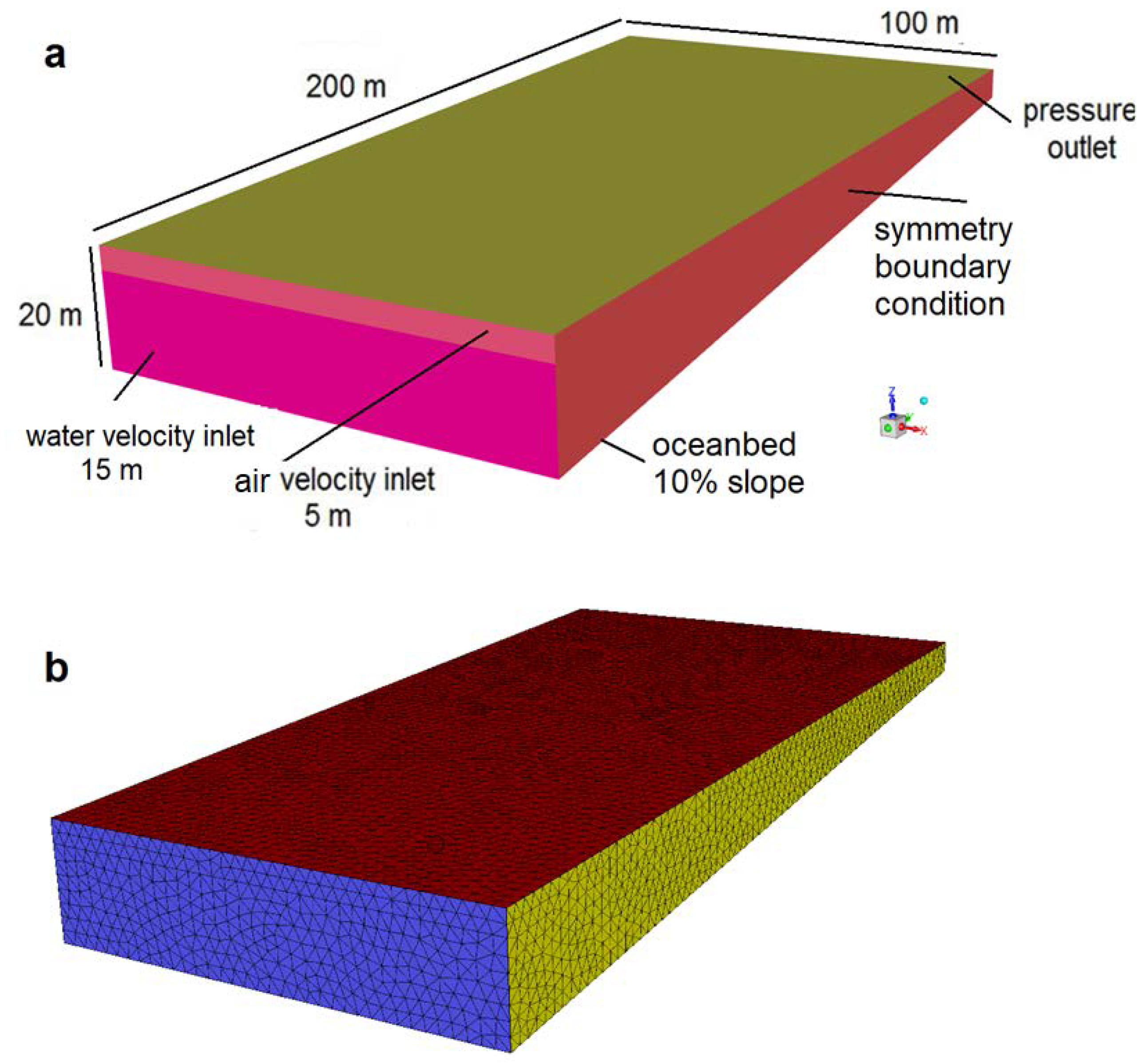
The geometrical model was based on a section of ocean near a coastal area with a length of 200 and width of 100 m, which was created and meshed using the SpaceClaim and Meshing packages, respectively, in Ansys Workbench 2020R1. The ocean bed slope was assumed to be 10% linear, so, at the distance of 200 m from the beach, the water depth was 20 m. Additional to this ocean section, a region with a height of 5 m above the oceanwater free surface level was also created to be as the atmosphere above the ocean filled with air. The grid independence test (GIT) was done for the five different meshes with sizes of 51,354, 89,487, 126,857, 215,312, and 323,564 cells. The independent analysis of the average velocity at the outlet revealed that the mesh with 126,857 tetrahedral cells and 24,384 nodes is sufficient for the mesh independency of the results. During the meshing process, the mesh quality was checked using a medium smoothing method. The mesh metrics for the optimum grid were in the acceptable range. For example, the average values of the element quality, skewness, aspect ratio, and orthogonal quality were 0.8169, 0.2519, 1.914, and 0.8431, respectively. The operating pressure of 101,325 Pascal was applied at the oceanwater surface, as well as a gravitational acceleration of 9.81 m × s⁻² in the downward Z direction.

Various boundary conditions were applied to the computational model. The ocean bed was designated as a stationary wall with no slip shear condition. The top surface of the model, as well as the beachside surface, were considered as the pressure outlet of the atmosphere. Two sides of the model were defined as symmetrical conditions, since the flow pattern for the other ocean sections near beach were expected to be symmetrical. The velocity inlet conditions were applied to the entries of the water and air currents from the oceanside. The geometrical model with labeled boundary conditions and the related computational grid are shown in Figure 1.

2.2. Volume of Fluid Model

The volume of fluid (VOF) model with a sharp interface modeling option was applied to account for an accurate interface transient tracking between two immiscible and non-interpenetrating fluids, where the volume fraction occupied by one of the phases in each cell can be computed and tracked throughout the Eulerian mesh [20]. The volume fraction of the qth phase in the VOF approach is denoted by ${\alpha }_q$. Therefore, when the control volume or cell is not occupied by the phase q, then ${\alpha }_q=0$ and, if completely occupied by that phase, then ${\alpha }_q=1$. Thus, for a cell containing an interface between the secondary qth fluid and one or more fluids, then $0<{\alpha }_q<1$. If there are two or more phases in the domain, then

$${\displaystyle \sum }_{q=1}^n{\alpha }_q=1$$

(1)

Interface tracking using the VOF method is accomplished by solving one continuity equation for the volume fraction. In order to determine the velocity field within the computational domain, a single momentum equation is also solved [8]. The continuity equation for the volume fraction of one or more of the secondary phases q is given as below:

$$\frac{1}{{\rho }_q}\left[\frac{\partial }{\partial }\left({\alpha }_q{\alpha }_q\right)+\nabla .\left({\alpha }_q{\rho }_q{\overrightarrow{\nu }}_q\right)=S_{\alpha q}+{\displaystyle \sum }_{p=1}^n\left({\dot{m}}_{pq}-{\dot{m}}_{qp}\right)\right]$$

(2)

where ${\dot{m}}_{pq }$is the mass transfer from the primary phase p to the secondary phase q, and ${\dot{m}}_{qp }$is the mass transfer from the secondary phase q to the primary phase p. The source term on the right-hand size is zero by default, but a user-defined value may be specified if necessary. The volume fraction for the secondary phase is determined from Equation (2); the volume fraction for the primary phase is not solved but, rather, determined from the constraint given by Equation (1). The volume fraction values are then used to calculate the volume-weighted averages for the density $\rho$ and viscosity $\mu ,$ which are used in the momentum equation given by Equation (3). The resulting velocity field is then shared among the phases to give the velocity of the secondary phase used in the continuity equation for the volume fraction above [21].

$$\frac{\partial }{\partial t}\left(\rho \overrightarrow{\nu }\right)+\nabla .\left({\rho }_q\overrightarrow{\nu }\overrightarrow{\nu }\right)=-\nabla p+\nabla .\left[\mu \left(\nabla \overrightarrow{\nu }+\nabla {\overrightarrow{\nu }}^T\right)\right]+\rho \overrightarrow{g}+\overrightarrow{F}$$

(3)

The properties in the above transport equations, i.e., density, pressure, and viscosity, are shared by the phases and are determined by volume-weighted averaging provided that the volume fraction of each of the phases is known at a particular location. The simple volume–fraction weighted average relationship given by Equation (4) is used to compute the weighted averages of the properties. Suppose that the phases are represented by subscripts (1) and (2), then:

$$\rho ={\alpha }_2{\rho }_2+\left(1-{\alpha }_2\right){\rho }_1$$

(4)

The volume fraction equation for the VOF model, given by Equation (2) above, is discretized by using either an implicit or explicit formulation. The robustness and stability of the implicit method makes it preferable and suitable for general purpose simulations involving transient calculations and was employed in the VOF simulations in this study.

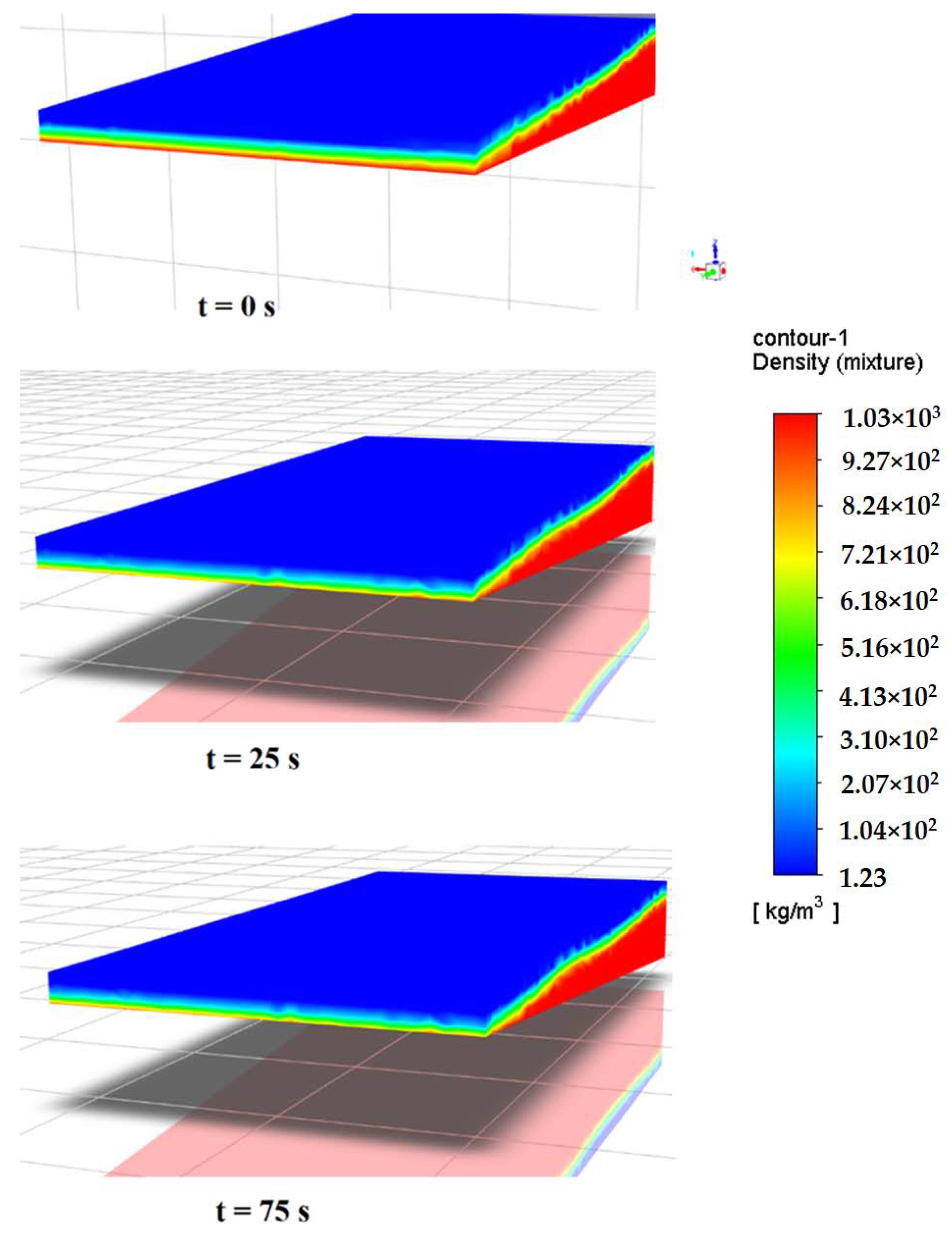
In this study, in order to consider the effect of wave propagation in the coastal marine environment, in addition to the VOF main model, the sub-models of the open channel flow and its wave boundary conditions (BC) were also included in the model setup. The air and oceanwater with densities of 1.225 and 1030 kg × m⁻³ were the primary and secondary Eulerian phases, respectively. The shear stress transport (SST) k-omega turbulence model was applied for the turbulence closure. It is the preferred model for VOF applications, as it supports turbulence damping in interfacial cells, which is critical for capturing interfacial instabilities.

As the VOF method is volume-conserved and computes and tracks the volume fraction of a particular phase in each cell rather than the interface itself, the level–set method was coupled to the VOF model to produce more accurate estimates of the interface curvature between two phases. In order to create irregular and random waves, a wind current with an air velocity of 10 m/s was defined as a breeze from the oceanside. This value is among the South African typical coastal wind speeds [22].

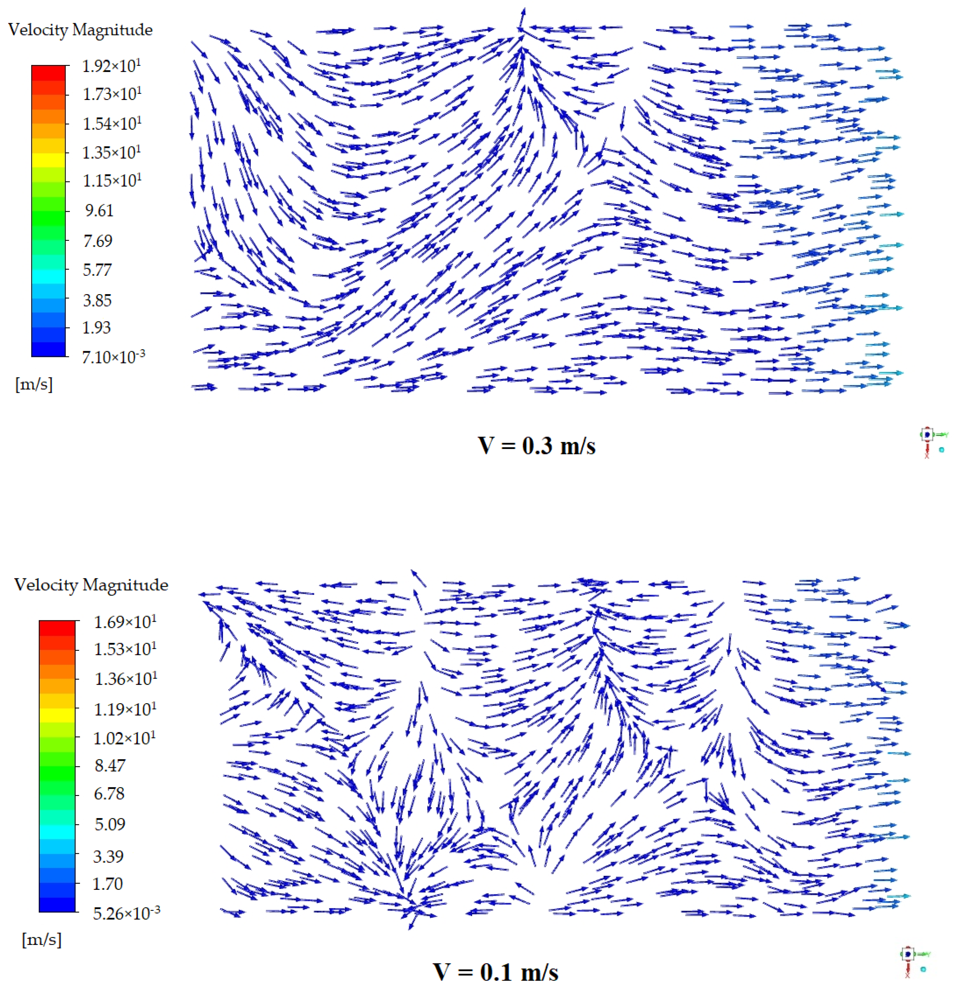
In order to study the effect of the oceanwater velocity on the distribution pattern of the particles, two flow velocity magnitudes of 0.1 m/s and 0.3 m/s were defined for the oceanwater toward the beachside in the Y direction at the water velocity inlet. These velocity magnitudes are in the typical range of water velocities for surficial currents and undercurrents near the coastal areas [23,24].

2.2.1. Open Channel Flows

Open channel wave boundary conditions are suitable for the purpose of a simulation of regular/irregular waves and allowed us to analyze the wave effects on microplastic particle motion and distribution. Ansys Fluent 2020R1 provided several different linear or nonlinear wave theories for the modeling of surface gravity waves in the boundary conditions of the velocity inlet type. The Ursell number is the decision parameter for choosing linear or nonlinear wave theories for shallow waves [21]. Some input parameters within the wave breaking and stability limit, as presented in the following sections, can affect the selection of the correct wave theory for a particular application.

The first-order Airy wave model, which is linear in nature, can be applied to small-amplitude surface gravity waves in coastal shallow liquid depth ranges.

2.2.2. Airy Wave Model

The following parameters need to be defined before describing the Airy wave model. The wave height H is defined as follows:

$$H=2A=A_t+A_c$$

(5)

where $A$ is the wave amplitude, $A_t$is the wave amplitude at the trough, $\mathrm{and} A_c$ is the amplitude at the crest. For the linear wave theory, $A_t=A_c,$ and for the nonlinear wave theory, $A_t\ne A_c.$The wave number (K) is:

$$K=\frac{2\pi }{\lambda }$$

(6)

where λ represents the length of the wave. The wave number K has a vector form as:

$$\overrightarrow{K}=K_x\widehat{x}+K_y\widehat{y}$$

(7)

where $\widehat{x}$ is the reference wave propagation direction, and $y$is the direction normal to $\widehat{x}$. Equations (9) and (10) give the wave numbers in the $\widehat{x}$and $\widehat{y}$directions, respectively:

$$K_x=K\cos \theta$$

(8)

$$K_y=K\sin \theta$$

(9)

$\theta$ is the wave heading angle, which is defined as the angle between the wavefront and reference wave propagation direction in the planes of $\widehat{x}$ and $\widehat{y}$. The effective wave frequency ${\omega }_e$ is defined as

$${\omega }_e=\omega +\overrightarrow{K}\times \overrightarrow{U}$$

(10)

where ω stands for the wave frequency, and $\overrightarrow{U}$ represents the mean velocity of the flow. According to the above parameters, the wave profile in the linear Airy wave model is given as [21]:

$$\zeta \left(X.t\right)=A\cos \alpha$$

(11)

α is a variable applied in all of the wave theories and is defined as:

$$\alpha =K_{x}x+K_{y}y-{\omega }_{e}t+\epsilon$$

(12)

where x and y are the space coordinates in the $\widehat{x}$ and $\widehat{y}$directions, respectively, ε is the phase difference, and t is the time.

2.2.3. Application of Wave Model and Formation of Wave Regime

In order to check whether the selected wave model is appropriate for the application, the following criteria were used:

Criteria applied to Complete Wave Regime inside Wave Breaking Limit:

The ratio of the wave height to depth of water $\frac{H}{h}$ for the wave breaking limit is given as:

$${\left[\frac{H}{h}\right]}_{max}=0.78$$

(13)

The ratio of the wave height to its length depth (known as wave steepness) inside the breaking limit is presented as:

$${\left[\frac{H}{\lambda }\right]}_{max}=0.142$$

(14)

Criteria applied to the wave theory within the wave breaking and stability limit:

For this purpose, a wave of a linear type can be represented with the suitable Airy wave theory. The following criteria are considered for this wave regime:

The ratio of the liquid height to wave length ($\frac{h}{\lambda })$for waves of a shallow depth is given as:

$${\left[\frac{h}{\lambda }\right]}_{max }=0.085$$

(15)

To check the wave steepness, the ratio of $\frac{H}{\lambda }$ for shallow waves is presented as:

$${\left[\frac{H}{\lambda }\right]}_{max }=0.02\tanh (2\pi \frac{h}{\lambda })=0.0156$$

(16)

To check the relative height, the ratio of $\frac{H}{h}$ for a linear wave is as below:

$${\left[\frac{H}{h}\right]}_{max}=0.1$$

(17)

The Ursell number stability criterion is defined as:

$$Ur=\frac{H{\lambda }^2}{h^3}$$

(18)

This criterion for a linear wave is given as:

$${\left(Ur\right)}_{max}=\frac{32{\pi }^2}{3}=105$$

(19)

In this study, for the water velocity inlet, a shallow/intermediate wave regime was applied as the appropriate boundary condition to model the surface gravity waves in the coastal ocean environment. The Airy wave model was also the selected method for this wave regime. The following values were used for the necessary input parameters in this wave model. These parameters were within the typical range of South African near-coastal conditions for the wave characteristics [25]:

• Significant Wave Height (H): 1.65 m,
• Wave Period: 10 s,
• Wave Length (L): 120 m,
• Water Depth (h) = 20 m, and
• Wave Heading Angle: 130 degrees.

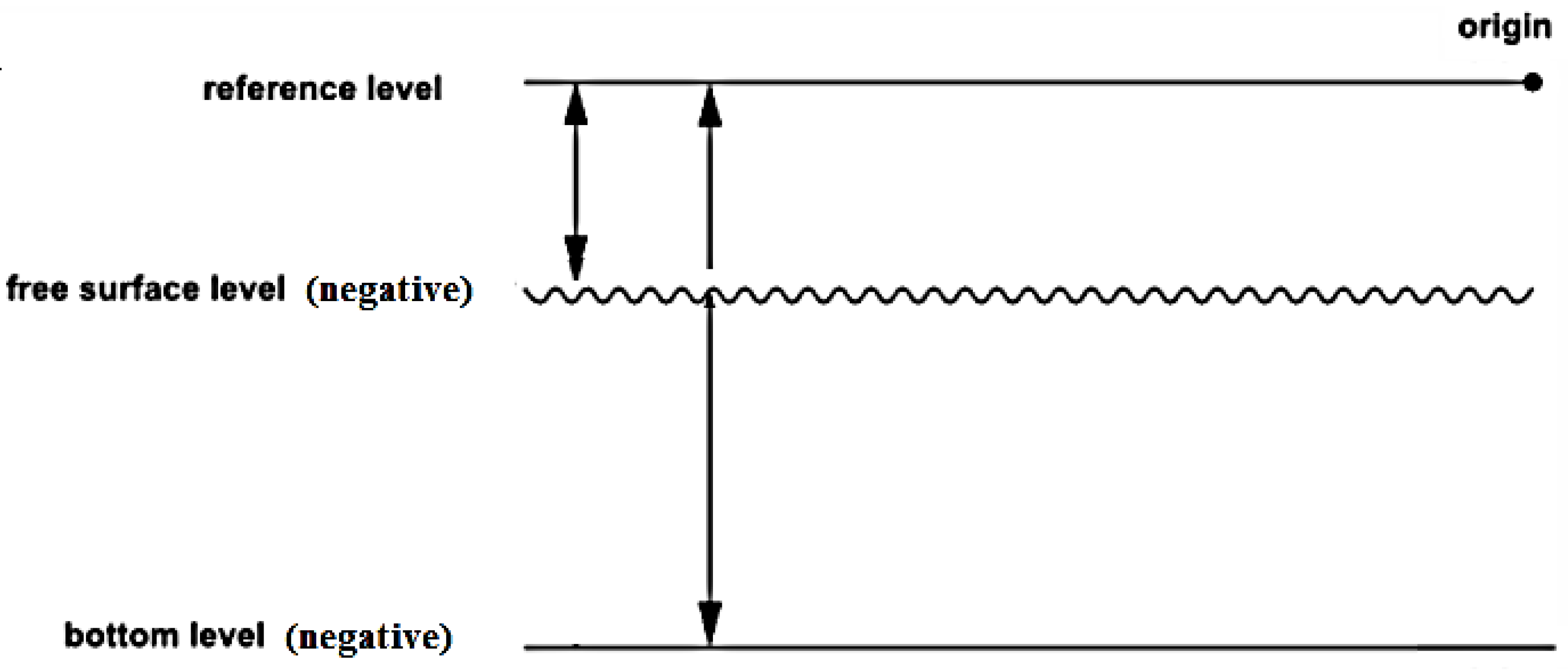
For the modeling of shallow and intermediate wave regimes, it is necessary to determine the free surface and bottom levels. Figure 2 illustrates the determination of the free surface levels for the open channel conditions.

According to the geometrical model in this study, and similar to Figure 2, the free surface level and bottom level were −5 and −25 m, respectively. The reference wave direction was computed based on the average flow direction. According to the wave input analysis based on the current settings selected for the velocity inlet, the Ursell number was equal to 2.97.

Criteria for the full wave regime in this study are summarized as:

The relative height (H/h) is equal to 0.0825 and is within the wave breaking limit (less than the theoretical maximum (0.78) and numerical limits (0.55)). The wave steepness (H/L) is equal to 0.0138 and is within the wave breaking limit less than the maximum theoretical (0.142) and numerical limits (0.12)).

The selected airy wave model parameters are also as follows:

• The relative height (H/h) is equal to 0.0825 and is within the minimum and maximum values of 0 and 0.1.
• The wave steepness (H/L) is equal to 0.0138 and is within the minimum and maximum values of 0 and 0.0156.
• The Ursell number (Ur) is equal to 2.97 and is within the minimum and maximum values of 0 and 105.
• For the wave regime check, the (h/L) is equal to 0.1667 within the minimum and maximum values of 0 and 10,000.

These successfully satisfied criteria showed that the selected wave model and wave regime were appropriate for application in this study. The numerical treatment of the beach conditions was activated for the whole fluid zone, as it can prevent the numerical reflection arising from the boundary of the pressure outlet while modeling surface gravity waves [21]. A one-dimensional option in the Y direction was selected for the damping type, and the computation was done from the water inlet boundary. In order to specify the damping length, the end point of 200 m with one wave length of 120 m was considered.

2.3. Discrete Phase Model (DPM)

The discrete phase model (DPM) follows the Eulerian–Lagrangian approach. In this approach, the fluid phase is considered a continuum, and the Navier–Stokes equations are solved, but the dispersed phase is solved by tracking the particles. The particle trajectories are predicted by integrating the force balance at specified time intervals during the fluid phase calculations. These particles can exchange the momentum, mass, and energy with a continuous fluid phase. The following equation is the particle force balance written in a Lagrangian reference frame:

$$m_p\frac{d\overrightarrow{u}}{dt}=m_p\frac{\overrightarrow{u}-{\overrightarrow{u}}_p}{{\tau }_r}+m_p\frac{\overrightarrow{g}\left({\rho }_p-\rho \right)}{{\rho }_p}+\overrightarrow{F}$$

(20)

where $m_p$is the particle mass, $\overrightarrow{u}$is the fluid phase velocity, ${\overrightarrow{u}}_p$is the particle velocity, $\rho$ is the fluid density, ${\rho }_p$is the density of the particle, $\overrightarrow{F}$ is an additional force, $m_p\frac{\overrightarrow{u}-{\overrightarrow{u}}_p}{{\tau }_r}$ is the drag force, and ${\tau }_r$ is the particle relaxation time [21].

The DPM model was applied to simulate the injection and transient tracking of microplastic particles with different types, sizes, and shapes. A single-point injection from the oceanside, 200 m from the shoreline, was selected as the site of an accidental spill that originated from a freight ship or a fishing boat. This point was considered as the source of entry of microplastics particles to the bulk ocean. The particles were injected into the domain at each fluid flow time step of 0.1 s and were also tracked unsteadily with the same time step size.

Suitable DPM boundary conditions of the “reflect” type were also applied to all surfaces, which keeps all particles available in the domain for the whole flow time simulation [26]. In these simulations, the interaction between the continuous phase and DPM particles was ignored due to the very low concentrations of particles in comparison with the volume of water. In other words, these simulations were one-way coupled. There were also no DEM collisions between the plastic particles, but the effects of the virtual mass, pressure gradient, and Saffman lift forces on the particle trajectories were included [27]. Three types of microplastic particles with different densities, sizes, and shapes were defined as given in

Table 1. Properties of the microplastic particles used in a numerical simulation.

Microplastic Type	Polyethylene Terephthalate (PET)	Polyurethane (PU)	Polypropylene (PP)
Density (kg · m−3)	1340	1120	900
Sizes (mm)	1, 5	1, 5	1, 5
Shape factors	0.1, 0.5, 1	0.1, 0.5, 1	0.1, 0.5, 1

.

Furthermore, in order to study the effect of particle shapes on the distribution pattern, two different drag laws of “spherical” and “non-spherical” with shape factors of 0.5 and 0.1 were used for each microplastic type with sizes of 1 mm and 5 mm. These drag laws are described in the next section. In Table 1, the value of 1 for the shape factor represents a spherical particle. The discrete random walk model (DRWM) or “eddy lifetime” model was used as the stochastic tracking method to include the turbulent dispersion of the particles [28].

With a combination of the above conditions for the particles, a total number of 18 different microplastics injections were designed to enter the domain from the oceanside. Each single injection of particles was defined with a constant flow rate of 0.01 kg/s for a duration of 5 s. Accordingly, a total mass of 0.9 kg consisting of about 794,000 microplastic particles in the form of 900 parcels was injected during the simulation.

2.3.1. Drag Models Used in the Simulations

There are several drag laws available in the framework of the Euler–Lagrange discrete phase model to determine the drag coefficient $C_D$. This coefficient is used in the calculation of the fluid drag force, which, in turn, is applied in the particle force balance or the equation of motion. The two spherical and non-spherical drag laws applied in this study are described below.

2.3.2. Spherical Drag Law

The drag coefficient $C_D$ for smooth particles can be taken from the following formula developed by Morsi and Alexander [29]:

$$C_D=a_1+\frac{a_2}{Re}+\frac{a_3}{R{e}^2}$$

(21)

where $Re$ is the relative Reynolds number, and $a_1$, $a_2$, and $a_3$are the constants that apply over several ranges of $Re$ given by Reference [29].

2.3.3. Non-Spherical Drag Law

For the non-spherical particles, Haider and Levenspiel developed the below correlation [30]:

$$C_D=\frac{24}{R{e}_{sph}}\left(1+b_{1}R{e}_{sph}{}^{b_2}\right)+\frac{b_{3}R{e}_{sph}}{b_4+R{e}_{sph}}$$

(22)

where

$$\begin{gathered} b_1=\exp \left(2.3288-6.4581\phi +2.4486{\phi }^2\right) \\ {b}_2=0.0964+0.5565\phi \\ {b}_3=\exp \left(4.905-13.8944\phi +18.4222{\phi }^2-1.2599{\phi }^3\right) \\ {b}_4=\exp \left(1.4681+12.2584\phi -20.7322{\phi }^2+15.8855{\phi }^3\right) \end{gathered}$$

(23)

The shape factor $\phi$ is defined as

$$\phi =\frac{s}{S}$$

(24)

where s is the surface area of a sphere with the same volume as the particle, and S is the actual surface area of the particle. For the purposes of calculating the particle mass, drag force, and $R{e}_{sph}$, the particle size should be the diameter of a sphere with the same volume. The shape factor cannot exceed a value of 1, which represents a spherical particle.

2.4. Energy Model

In order to investigate the effect of oceanwater temperature on the distribution of the particles, an energy equation was enabled, and new properties such as the thermal conductivity and specific heat capacity were defined for all three plastic types. These values are given in

Table 2. Thermal properties of the microplastic particles used in the numerical simulations.

Microplastic Type	PET	PP	PU
Specific heat capacity	1120	1900	1580
Thermal conductivity (W/m.°C)	0.144	0.218	0.24

.

When small particles are suspended in a fluid that has a temperature gradient, they experience a force in the direction opposite to that of the gradient, which is called the thermophoretic force. This phenomenon is known as thermophoresis or thermomigration, which is observed in mixtures of mobile particles where the different particle types exhibit different responses to the force of a temperature gradient [31]. This thermophoretic effect was also included here on the particle force balance equation.

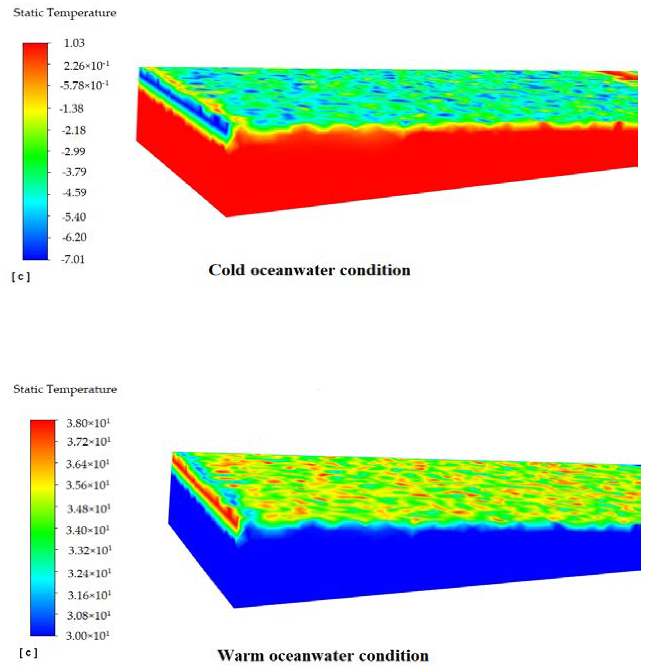
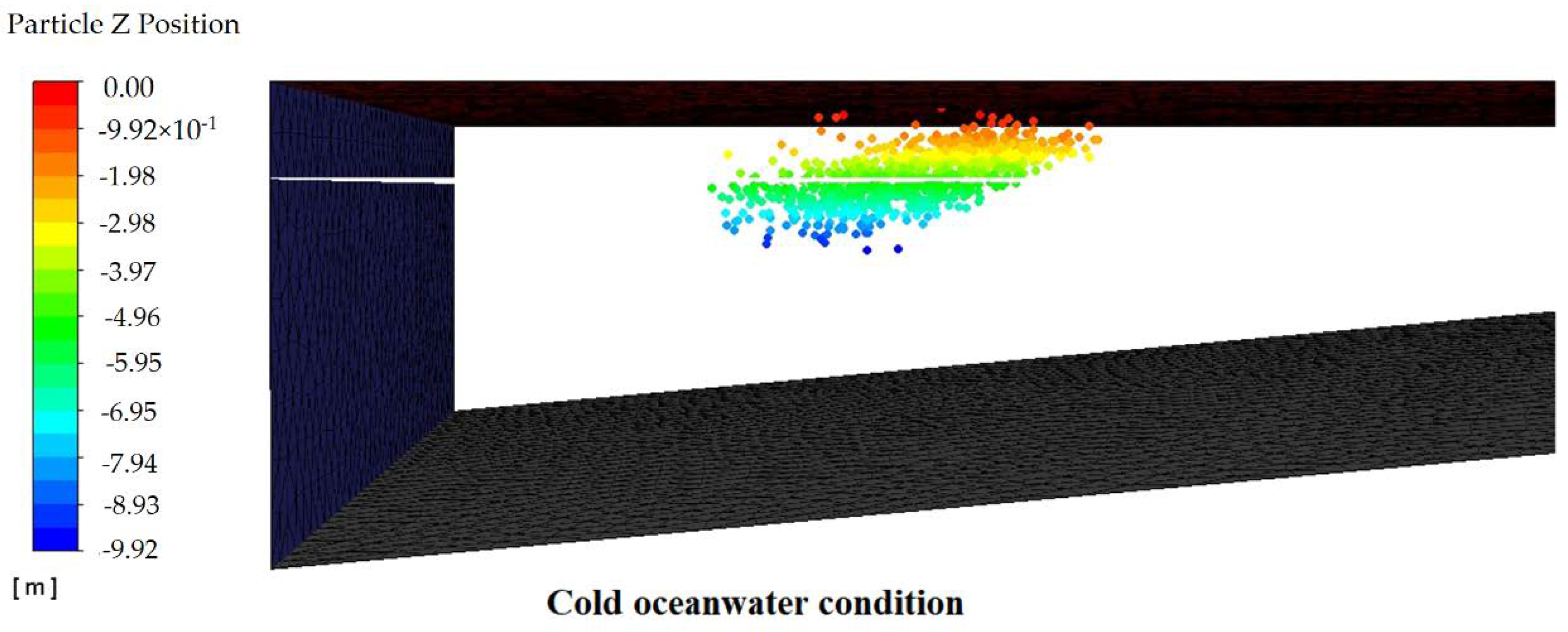
According to the available data about the temperature of oceanwaters globally, two different temperatures of 30 and 1 °C were selected for the oceanwater zone to represent two opposite conditions of warm and cold weather. The temperatures of the air at the inlet and outlet above the oceanwater were also adjusted based on the weather conditions. For cold and warm weather conditions, the temperatures of the air were assumed to be −7 and 38 °C, respectively. The initial temperature for all the particle injections was also set to 5 °C. In order to save more computational time, two comparative simulations were carried out for a flow time of 20 s.

2.5. Computational Method

The calculations were performed using Ansys Fluent 2020R1 in an unsteady solution mode with a double-precision, pressure-based solver. The bounded second-order implicit was selected for transient formulation. The Pressure-Implicit with Splitting of Operators (PISO) algorithm was used for pressure–velocity coupling with PRESTO (PREssure STaggering Option) and compressive schemes for obtaining the pressure and volume fractions, respectively. The second-order upwind scheme was also considered for the momentum, turbulent kinetic energy, specific dissipation rate, and level–set function.

After initialization of a solution from all zones with the wavy method of open channel initialization, the volume fraction of the water phase for the specified oceanwater zone was patched to 1. A time step of 0.1 s with a maximum of 10 iteration per time step was found to be sufficient for the stability and maintenance of numerical solution convergence at every time step. The convergence of a numerical solution was determined based on the surface monitoring of integrated quantities of the bulk flow velocity and turbulence and scaled residuals of the continuity; x, y, and z velocities; k-omega, and volume fraction of the water. The residuals of all the quantities were set to 10⁻³, and the solution was considered converged when all the residuals were less than or equal to the set value. Simulations were run for a total flow time of 5 min at a computational time of 10 h using 4 parallel 2.6 GHz CPU cores and 8 GB RAM.

3. Results and Discussions

3.1. Fluid Flow Characteristics

The density contours of the mixture phase for the case of an oceanwater velocity of 0.3 m/s at different simulation times are shown in Figure 3.

At zero time, the water free surface is in its initial conditions, but with entering the water from the related velocity inlet boundary, an increase in the oceanwater free surface level is seen, and the surface gravity random waves are created at the water–air interface, which move towards the beach because of the prevailing wind direction from the ocean. When the water surface waves approach the beachside, the water level decreases due to the damping effect of the waves.

The velocity vectors shown in Figure 4 demonstrate the mixing behavior of the flow at the bottom of the domain (namely, ocean bed) due to the existence of undercurrents and the effect of the wave motions for two different water velocities of 0.3 m/s and 0.1 m/s. It can be seen that, in the case of the lower velocity, more mixing undercurrents existed. These mixing flows plays a significant role in the trajectory of microplastic particles, and they may experience different motions: backward, forward, and rotational.

3.2. Microplastic Particle Dispersal

3.2.1. General View of Microplastic Traces

Figure 5 and Figure 6 display the snapshots of simulated traces for all types of microplastic particles in the oceanwater velocities of 0.1 m/s and 0.3 m/s, respectively, after 5 min colored by the location density. The red particles are those already sinking into the water, and the yellow to light blue particles are those floating on the water surface. These figures provide a general view of the distribution pattern for different particles, where the noticeable differences between their dispersion due to the influence of the plastic type and water velocity are observable. It is clear that, in the higher velocity of 0.3 m/s, some of the particles from all types reach the beachside. In order to make a better understanding of the particle motions and an easy quantitative comparison between the water depths and distances traveled by different particles, some distribution graphs in two vertical and horizontal directions were created from the particle stream position data in postprocessing, which are presented in the next sections.

3.2.2. Vertical Distribution Charts

In the vertical distribution charts, the percentage of particles that are floating or sinking in different water depths are given based on their type, size, and shape. The water depths were defined in three levels of 0–5, 5–10, and below 10 m. The floating particles were identified based on their current location density, as shown in Figure 5 and Figure 6. From these charts, it is possible to have a comparison between the effect of each parameter on the distribution pattern and find the main significant parameters.

Figure 7 presents the vertical distribution for microplastic particles traveling at a water velocity of 0.1 m/s. It is clear that, for both PET and PU particles, the majority of them were sinking in depths of 10 m from the water surface or already settled at the ocean floor. For both large 5-mm PET and PU, the percentage of particles at a water depth of 10 m increased as the particle shape factors increased from 0.1 to 1, showing the effects of the particle shape. Additionally, for small 1-mm particles with a 0.1 shape factor, about 14% floated between the surface and a bulk water column of 5 m, as compared to only 4% of the spherical counterparts. As the size and shape factors increased, the particle shape was closer to the sphere, and the microplastic particle count in depths below 10 m increased, indicating the tendency of smaller non-spherical shapes for the increased buoyancy. For PU non-spherical particles, a similar trend was also visible, but the percentage of particles floating in the bulk water was greater than that of the PET particles due to PU having a lower density than that of PET.

In the case of PP particles, as expected, most of the particles are moving in near-surface depths of 0–5 m due to their lighter density. For spherical particles of 5 mm, all of the particles float between the water surface and 5 m in contrast to 66% of the 1-mm particles, the rest of which are 10% floating on the surface, 18% between 5 and 10 m, and 6% sunk to the bottom. Non-spherical particles of a 0.1 shape factor depict a completely different picture in which the size effect becomes less important, and on average, 65–70% of the particles floating in the bulk water between the surface and 10 m, 10% floating on the surface, and 20% are already sunk to the sea floor. For non-spherical particles with a 0.5 shape factor, again, a high percent of them travels in near-surface depths, and the others are in deeper levels. Approximately 10% of PP particles of 1–5 mm of all the shapes float on the water surface, which is greater than those of PET and PU particles.

Figure 8 shows vertical distribution charts for microplastic particles for a 0.3 m/s water velocity. In these charts, the percentage of the particles in each water depth level is different from the charts in Figure 7 because of the higher water flow velocity influence on the particle dispersion.

In the case of spherical PET, 100% of the large 5-mm particles have sunk to below 10 m or at the bottom of the sea due to their higher mass compared to the small particles, of which only about 40% are at those depths due to higher water flow velocities providing smaller particles less opportunity to settle down to deeper levels. Non-spherical large 5-mm particles with shape factors 0.5 and 0.1 show that approximately 50 and 15% sank below 10 m as compared to the spherical counterpart. For non-spherical small 1-mm PET particles, the influence of the shape factor was more pronounced in that only about 15% sunk below 10 m. Similar trends were observable for the PU microplastics in Figure 8. At a 0.3 m/s water velocity, the PP particles demonstrated that the shape factor does not play an important part in the float–travel–sink interplay, and interestingly, almost independent of the shape and size, around 30–40% of the floating on the water surface and most of the rest are situated between the surface and a 5-m depth.

3.2.3. Horizontal Distribution Charts

In these distribution charts, the horizontal distances traveled by different particles toward the beach were measured in three different ranges of 0–50, 50–100, and 100–200 m based on their tracking data.

Figure 9 presents the horizontal distribution charts for all microplastic particles, where the water velocity is 0.1 m/s. It can be seen that most of the PET and PU particles were scattered into two distance ranges of 0–50 and 50–100 m, and those particles traveled for longer distances up to 200 m (reporting on the shoreline), limited to a maximum of 12%. However, 100% of 5-mm spherical and 76% non-spherical with a 0.5 shape factor mainly traveled a maximum distance of 50 m, while about 60% of the 5-mm non-spherical particles with a 0.1 shape factor traveled further, between the 50 and 200-m range. For small 1-mm particles, approximately 90% traveled up to 100 m, which is distributed evenly for different shape factors. The rest traveled about 10% further to 200 m, which was the shoreline. The fraction of PU particles for longer distances travel in all classes was also comparatively more than that of the PET particles, probably owing to its lower density.

In the case of PP particles, it is obvious that longest travels were achieved by the ones with spherical shapes; 84% of the small and 100% of the large particles traveled between 50 m and the shoreline. Moreover, 40% of the 5-mm spherical-shaped particles reached the shoreline, and 60% traveled between 50 and 100 m in range. For non-spherical small particles. the results revealed that a maximum of 22% reached the shoreline as compared to only 14% of the large 5-mm ones. This shows that there is an interplay between shape and size for non-spherical PP particles in terms of distribution, while, at the same time, spherical particles showed that the larger ones traveled farthest with a 0.1 m/s water velocity, which was a completely different scenario in the case of 0.3 m/s, as can be seen in Figure 10.

Figure 10 illustrates the horizontal distribution for all microplastics in the water velocity of 0.3 m/s. As expected, a totally different pattern was seen since increasing the oceanwater velocity compelled the particles in all the streams to travel longer distances. For PP particles, more than 90% reached the shoreline independent of the shape and size. For the PET non-spherical particles, approximately 80% of the small and 70% of the large ones were reported on the beach. For the spherical 5-mm particles, only 2% traveled to the shoreline compared to 72% of the 1-mm ones. Around 70% of small non-spherical PU particles and 65% large non-spherical PU traveled 100–200 m in comparison with the spherical small ones (about 50%) and large ones (about 30%), respectively. This indicates that, in fast-moving waters with a 0.3 m/s velocity towards the shoreline, non-spherical particles travel faster for heavy particles like PET and PU. However, in the case of lighter microplastics, the PP size and shape effect disappear, and almost all particles reach the shoreline and will be distributed along the beach.

3.2.4. Effect of Oceanwater Temperature

The static temperature contours for the mixture phase after 20 s in both cold (1 °C) and warm (30 °C) conditions of oceanwater with a speed of 0.1 m/s are shown in Figure 11. This figure shows the static temperature variations inside the computational domain, and the differences between the oceanwater and surrounding air temperature in both climate conditions are clear. The air temperature at the air inlet was set equally 8 °C colder and warmer than the oceanwater phase. It is seen that the main variations in temperature occur at the water surface and the air zone above it. The water temperature below the ocean surface remains constant for both temperature conditions.

The particle traces for both thermal conditions were identical as the temperature of the oceanwater had no specific effect on the movement and distribution patterns of all the microplastic particles of different types, sizes, and shapes, and the particles moved in both conditions similarly. The results of particle tracking for cold oceanwater conditions colored by the Z position are shown in Figure 12. From this figure, it can be seen that, 20 s after an injection, the maximum depth that these particles sunk to was about 5 m, with a travelling distance range of up to 50 m.

4. Conclusions

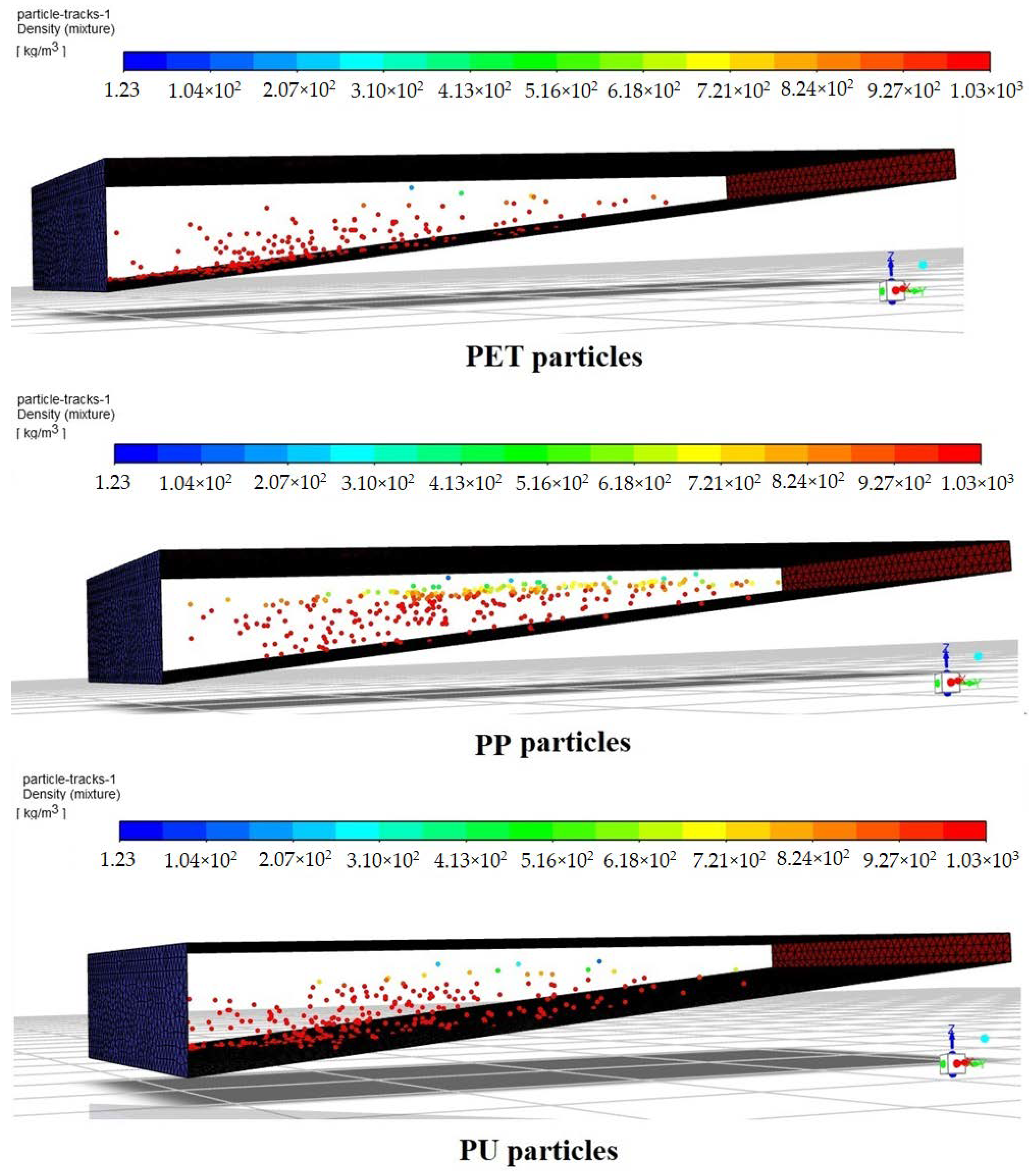
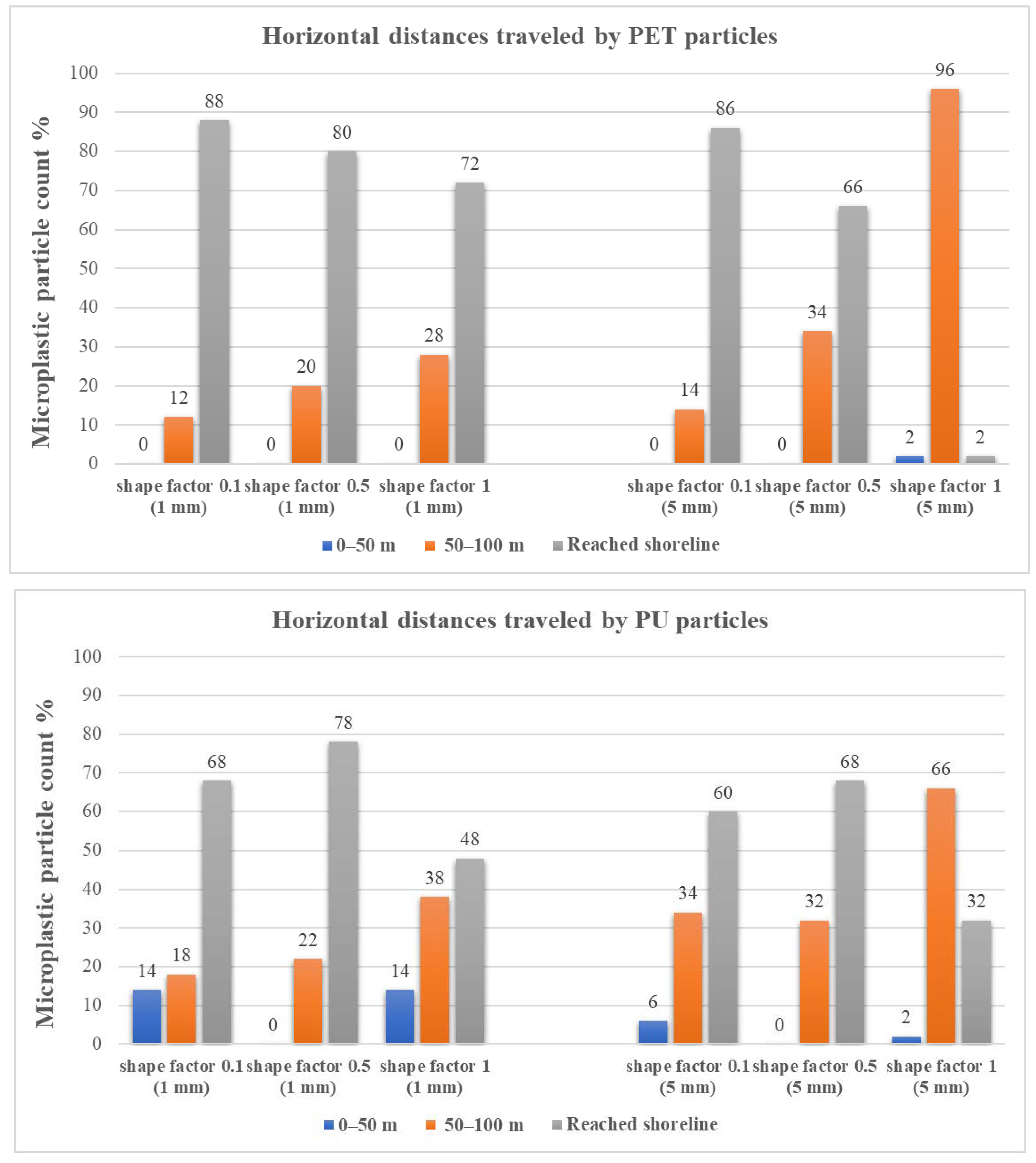
In this study, CFD numerical simulations were carried out by applying multiphase VOF model, Open Channel Flow, DPM and Energy models to investigate the effects of various variables on microplastics motion and distribution in simulated near coastal conditions. Eighteen different microplastic particle streams consisting PET, PU and PP of different size and shape were released from a single point in the coastal waters simulated using Airy wave theory with input wave characteristics from a real case study. Simulations were run for 5 min flow time with two different oceanwater velocities and temperature conditions and the particles were tracked to investigate the effect of physical properties such as shape and size.

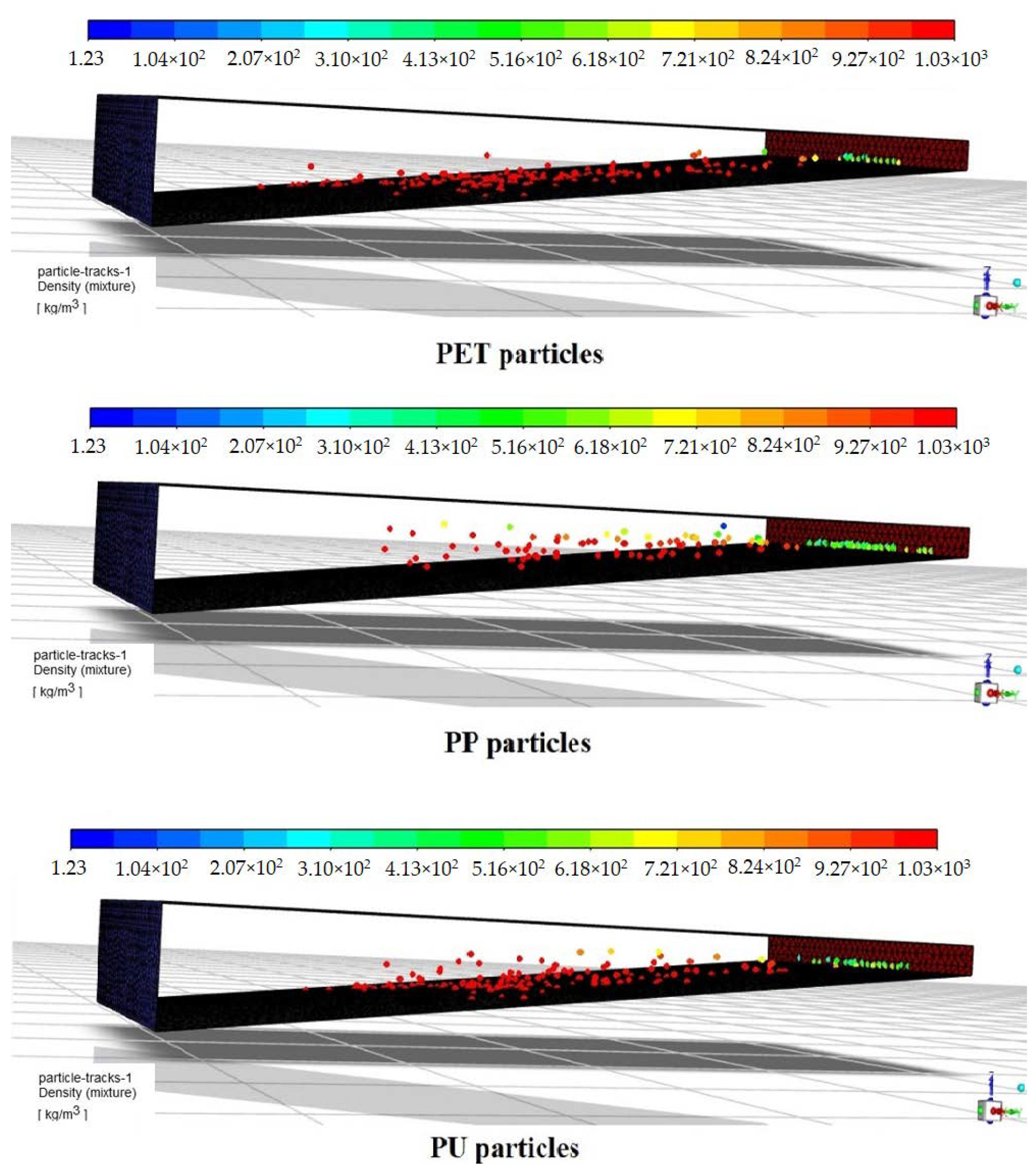
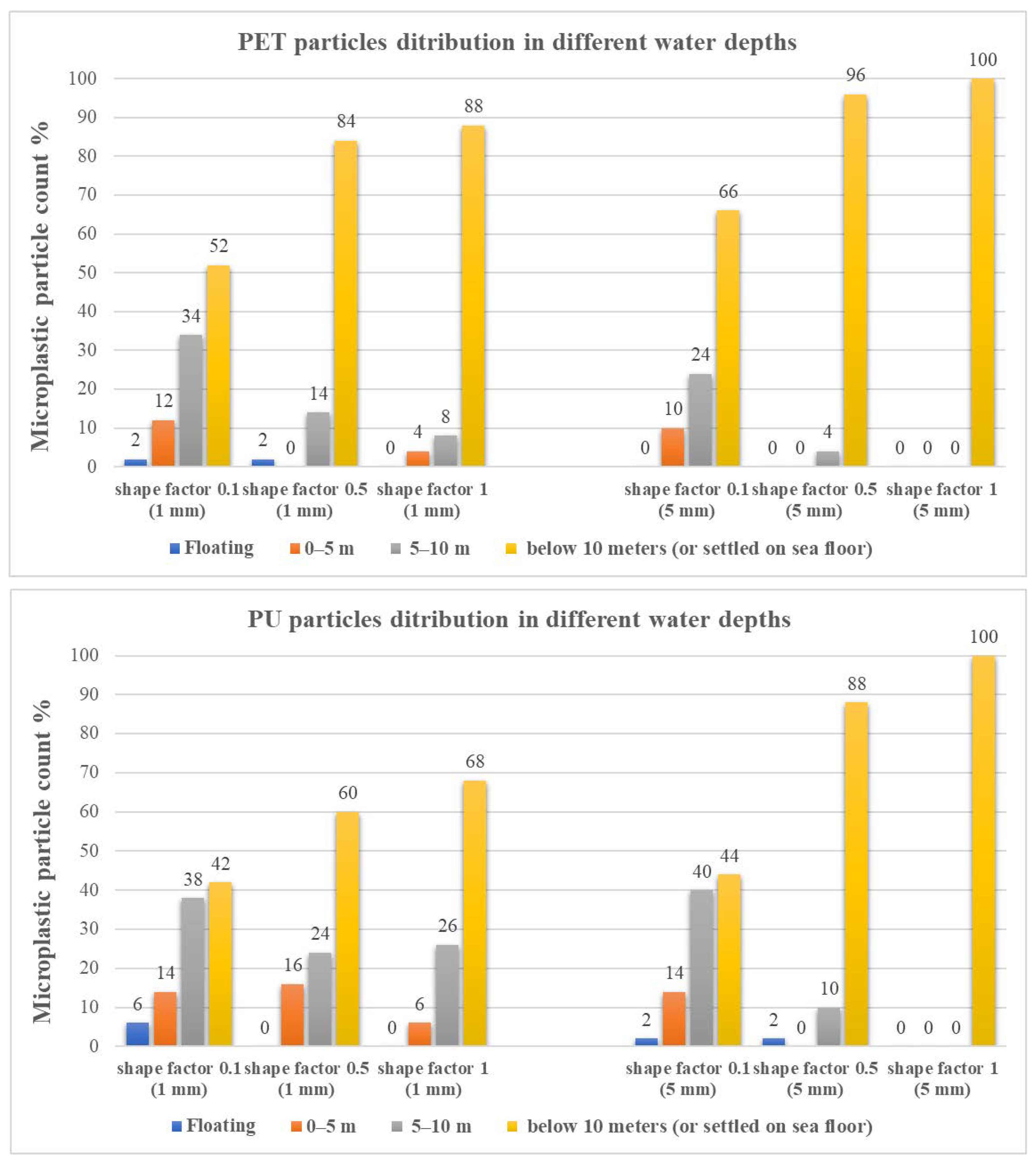
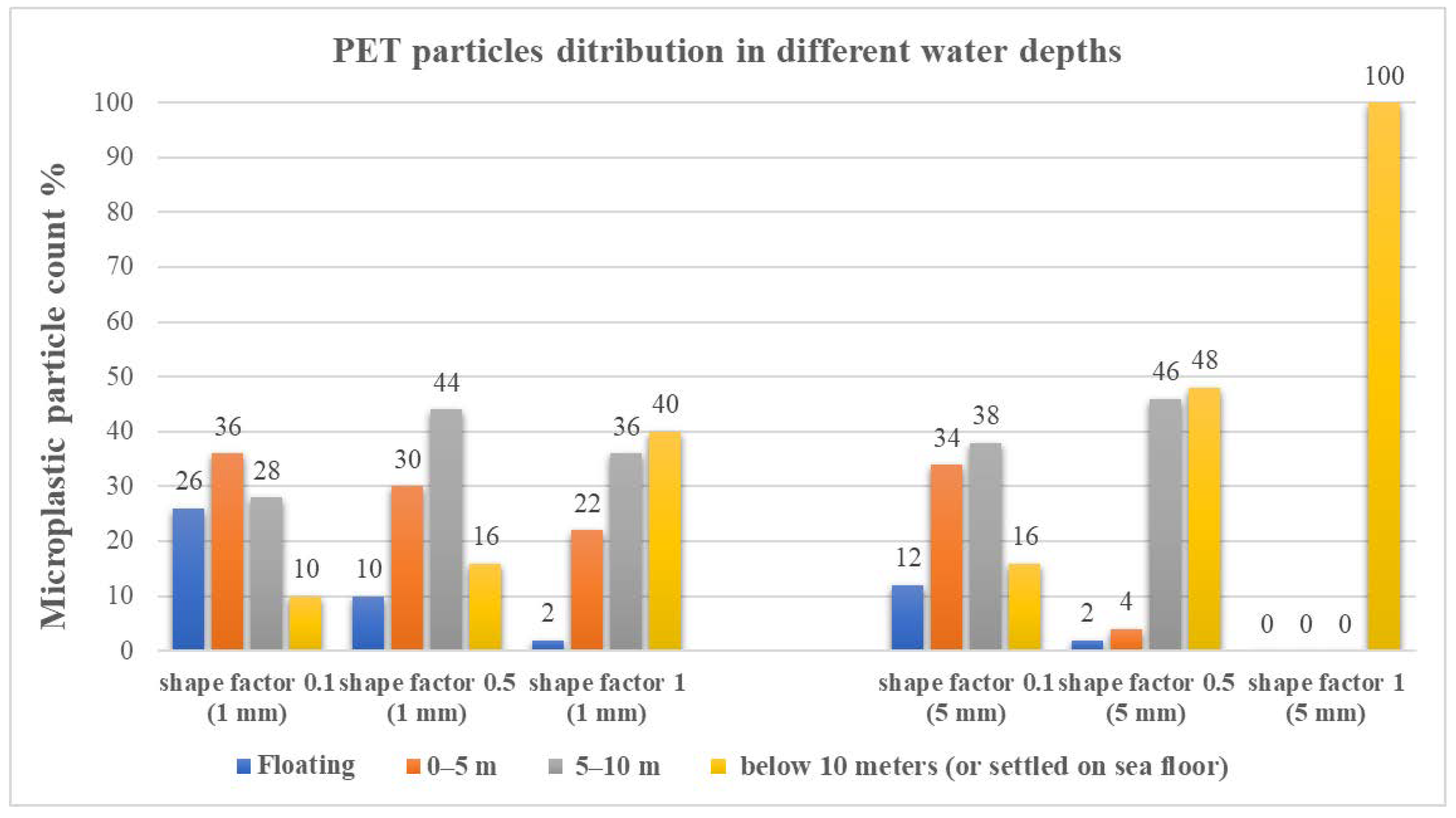
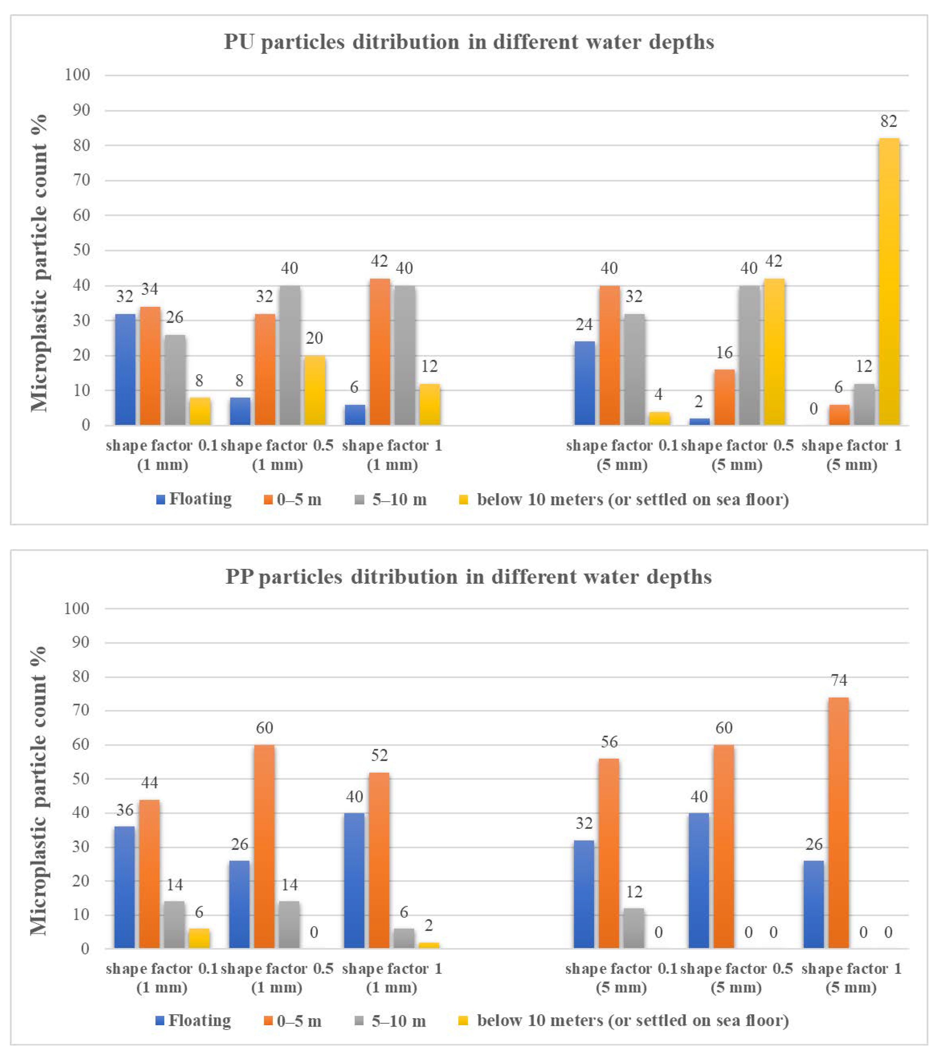
Particle tracking results were used to determine the effect of each parameter on particles travel pattern. The spatial distribution of particles in each simulation case were compared and revealed that with low water velocity the most of large denser spherical PET and PU microplastics settle at the ocean floor while the small non–spherical particles travel near the surface towards the shoreline. This finding seems to be in line with Alsina et al. (2020) who observed a large influence of the particle density causing particles to float or sink for relative densities lower and larger than water respectively. They found that the measured net drift of the floating particles correlated well with Stokes particle drift velocity. They argued that floating particles remain at the free water surface because of buoyancy and non-floating particles move close to the bed with lower velocity magnitudes than those of the floating particles.

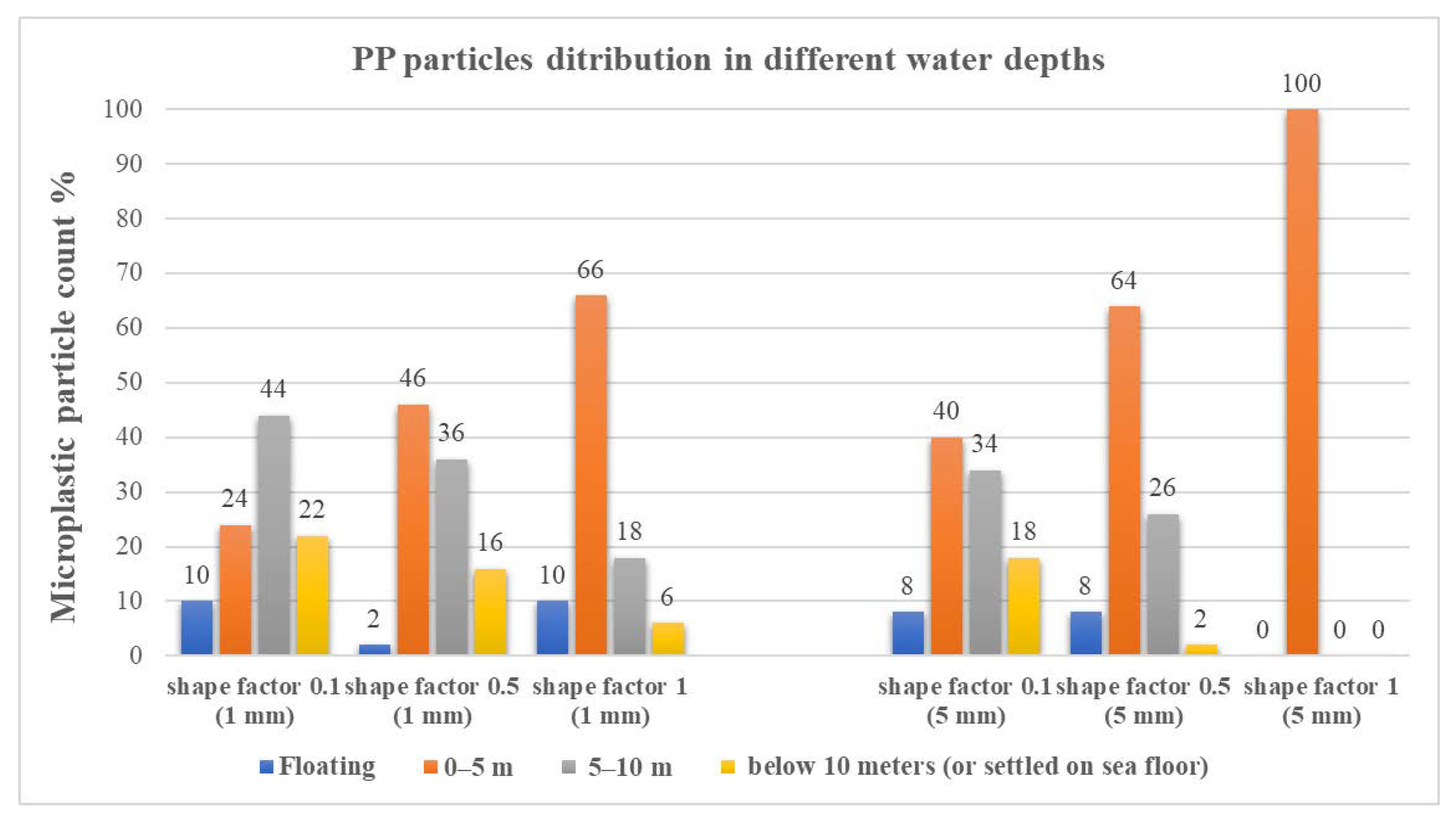
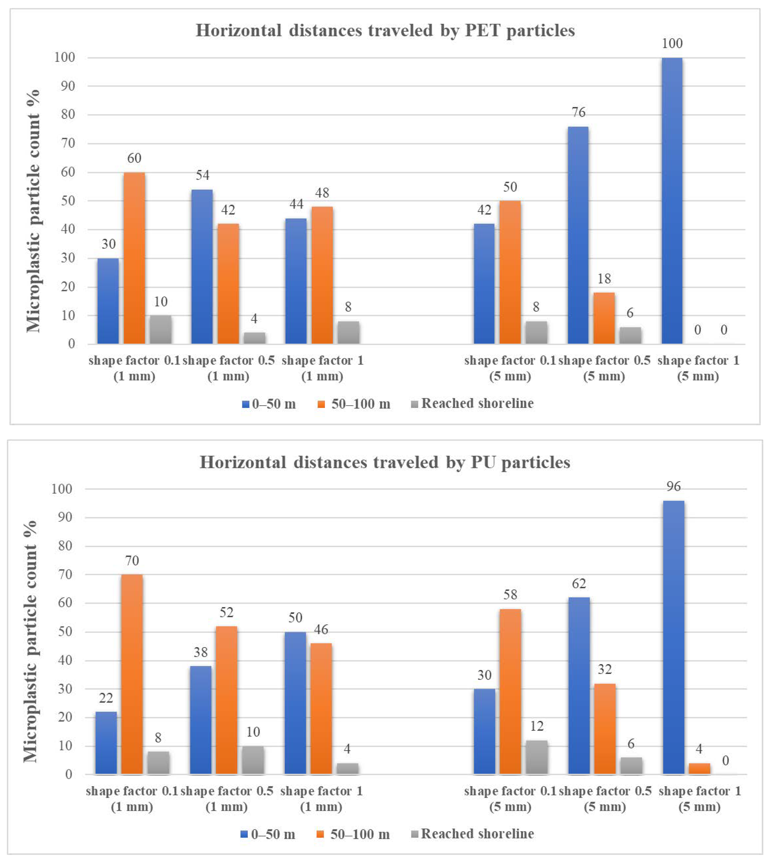
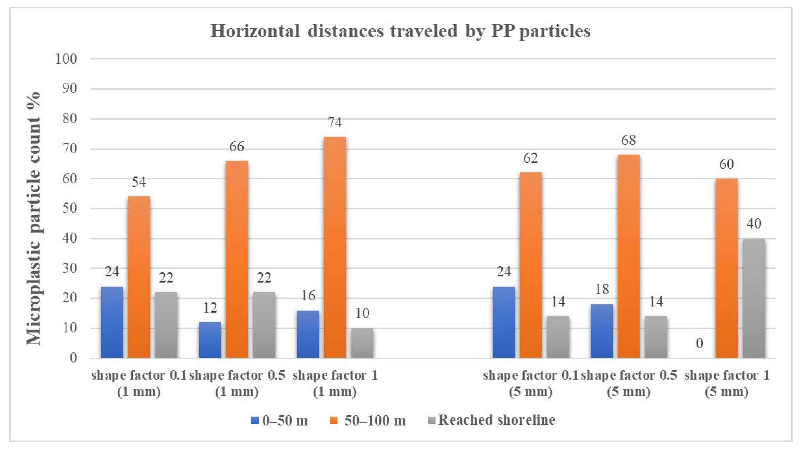
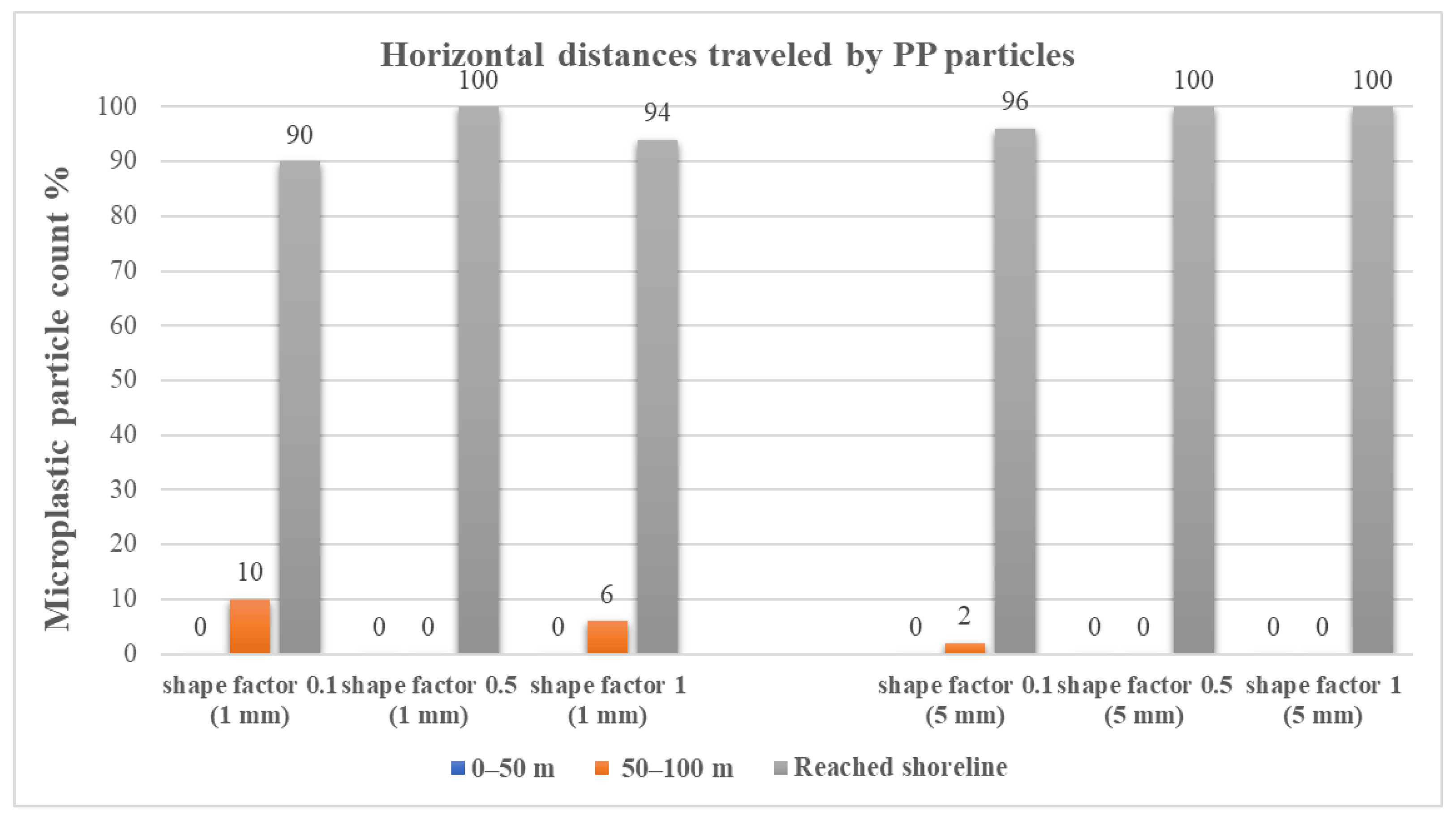
The results also reveal that lighter PP microplastics larger spherical particles float more easily than denser spherical ones. Large spherical and smaller non–spherical PP particles travel fastest and transport to the shoreline. With increasing water velocity lighter PP particles, almost independent of shape and size, travel farthest to the shoreline together with smaller non–spherical denser microplastics. Forsberg et al. (2020) found that plastic properties, shape, and density, govern the behavior of plastic litter in the nearshore zone. Kerpen et al. (2020) also found that denser microplastic particles have been partly confined into deeper layers of the sloping beach and particles with a low density floated in the surf zone or deposited on the beach. Ho and Not (2019) reported that the preferential accumulation observed at the inner boundary between the beach and breaking zone is related to physical characteristics of the plastic pieces.

In summary, along the shoreline one would observe that most of the microplastics are lighter PP particles relatively independent of shape and size with some small denser particles of PET and PU distributed along the beach.

Lastly, the simulation results revealed that the oceanwater temperature did not play a significant role in the spatial distribution of microplastic particles.