
Visual Harmony of Engineering Structures in a Mountain Stream


Abstract
:1. Introduction
1.1. Visual Harmony
1.2. Aesthetic Assessments of Rivers
1.3. Objectives of This Study
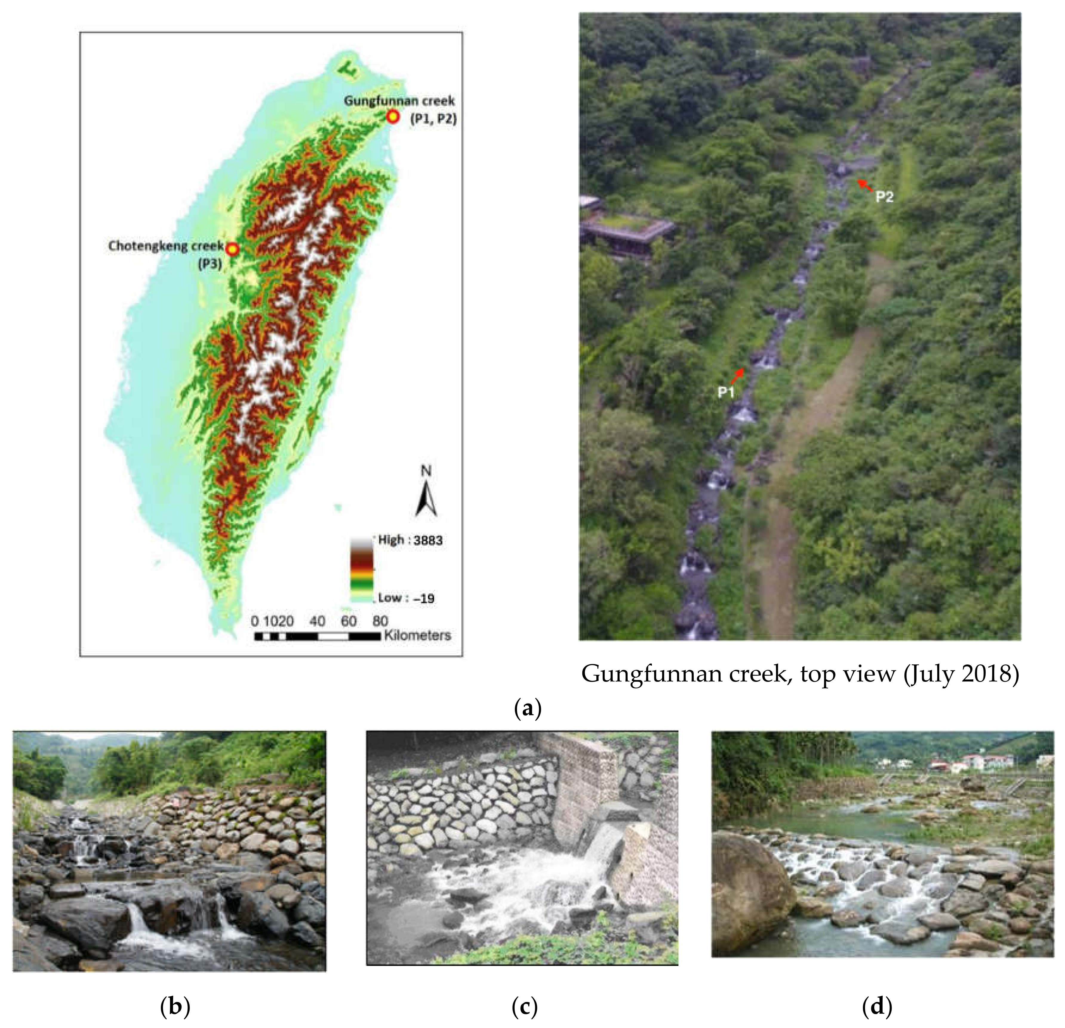
2. Overview of Gungfunnan, Chotengkeng, and Tungsikun Creeks
3. Methods
3.1. Image Collection and Processing
3.2. Calculating the Physical Elements Using the Four Visible Indicators
3.3. Questionnaire Survey
3.4. Results Presentation
4. Results and Discussions
4.1. Harmony
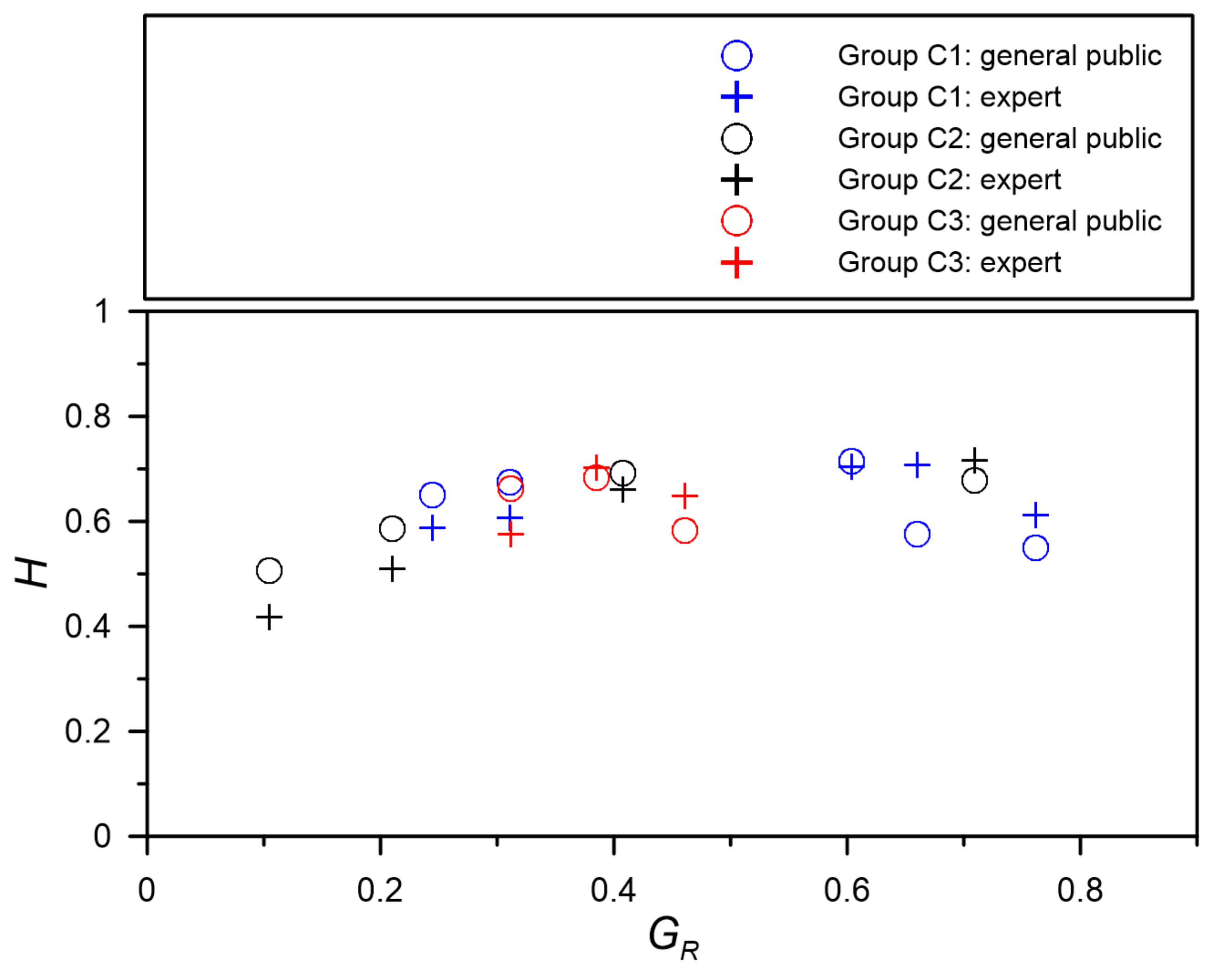
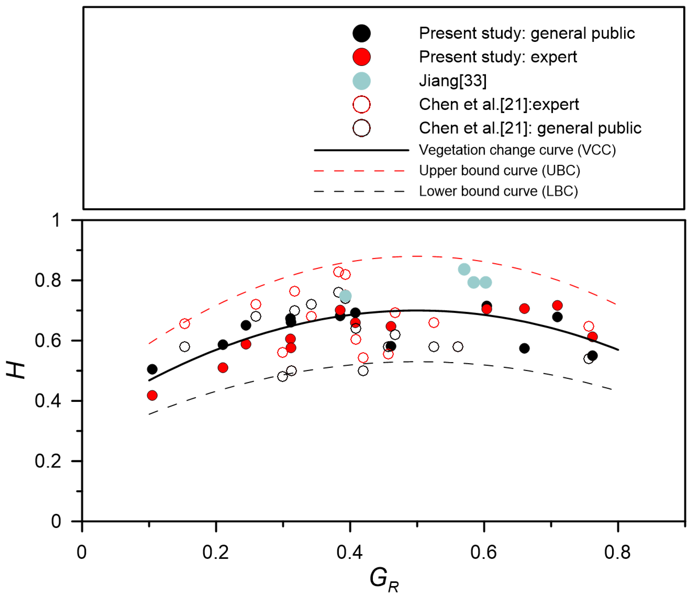
4.1.1. Visual Harmony and Visible Greenery
4.1.2. Factors Affecting the Harmony and Visible Greenery Relationship
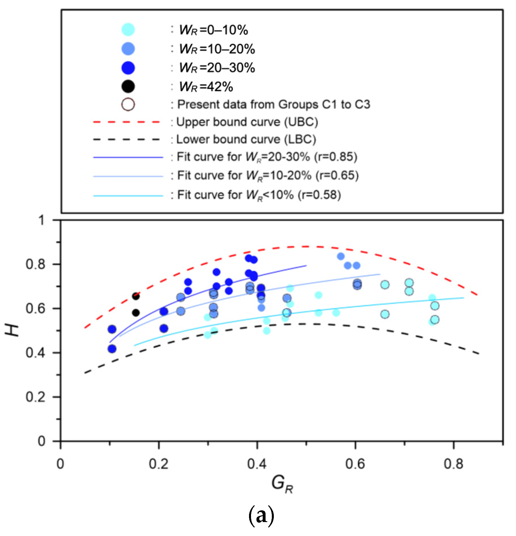
- (1)
- Water amount
- (2)
- Proportion of structure
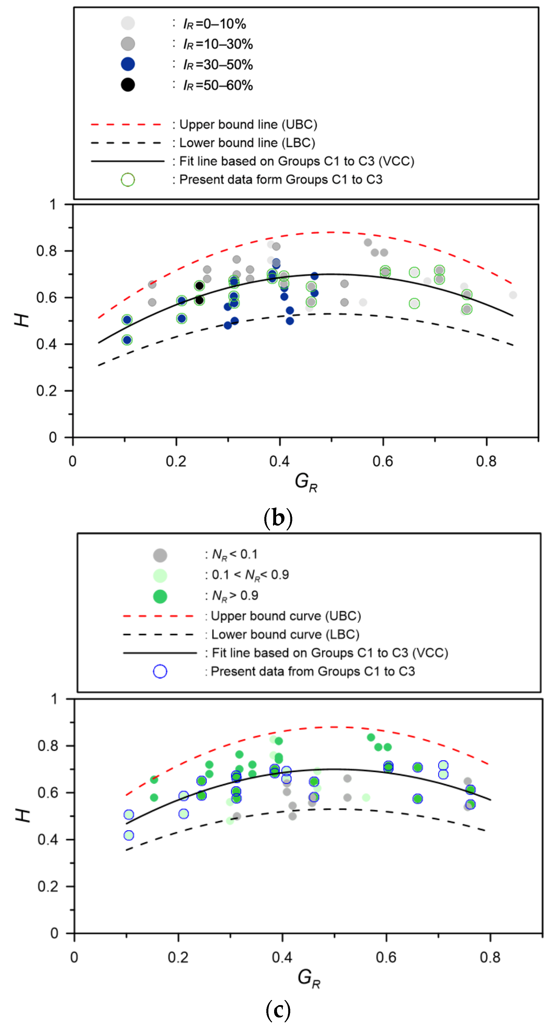
- (3)
- Materials on the surface
4.2. Visual Preference
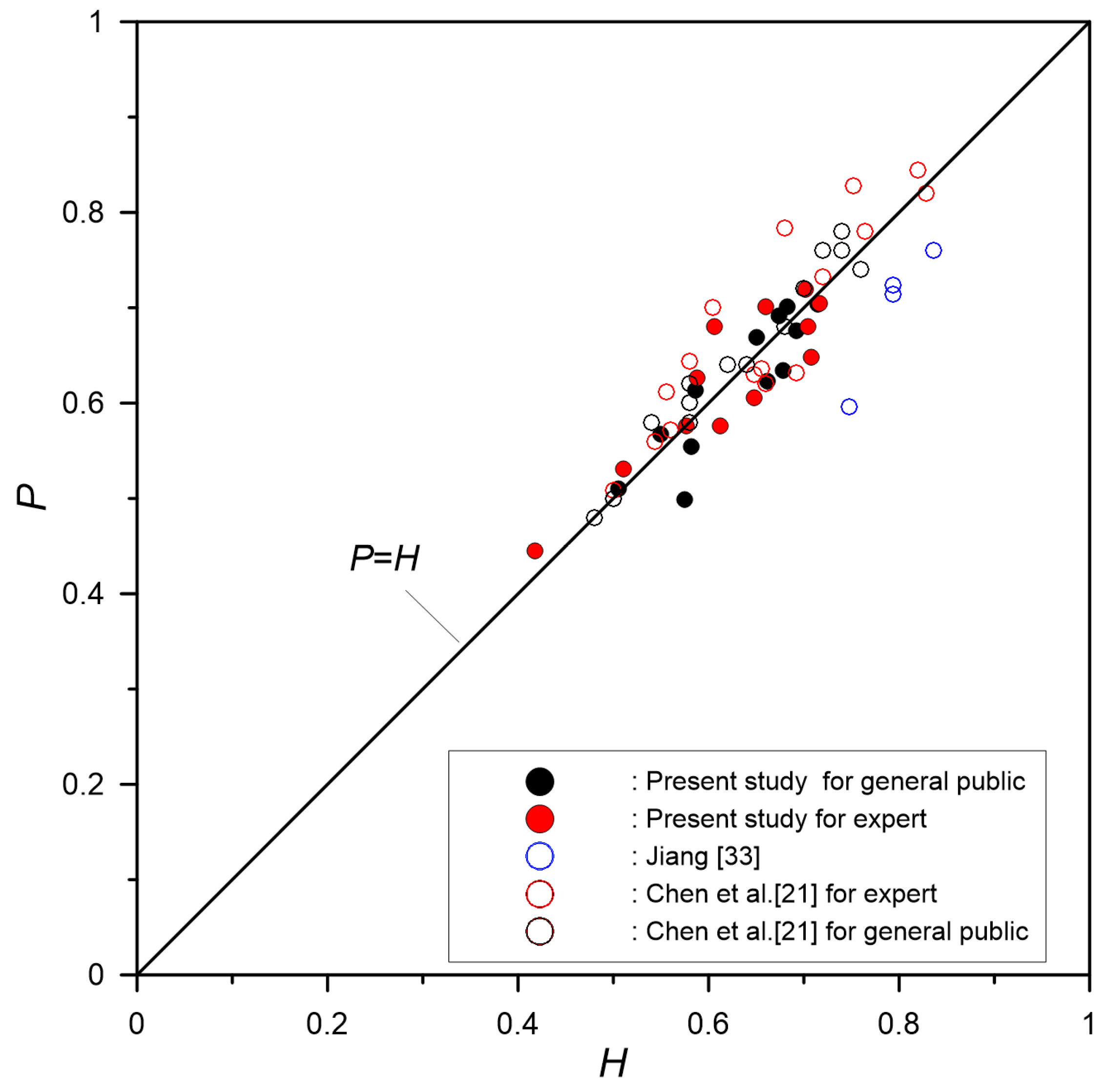
4.2.1. Relationship between Visual Preference and Harmony
4.2.2. Factors Affecting the Visual Preference and Visible Greenery Relationship
4.3. Model Using the Combined Physical Indicator M
5. Conclusions
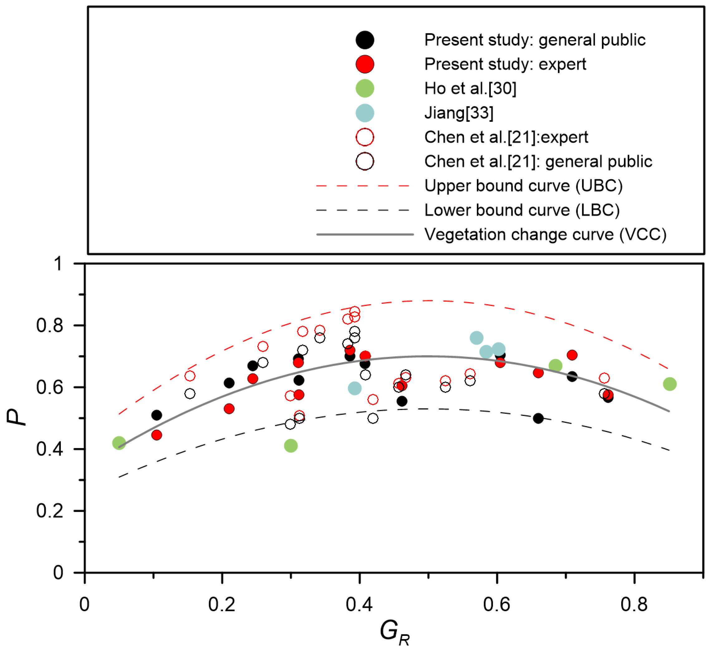
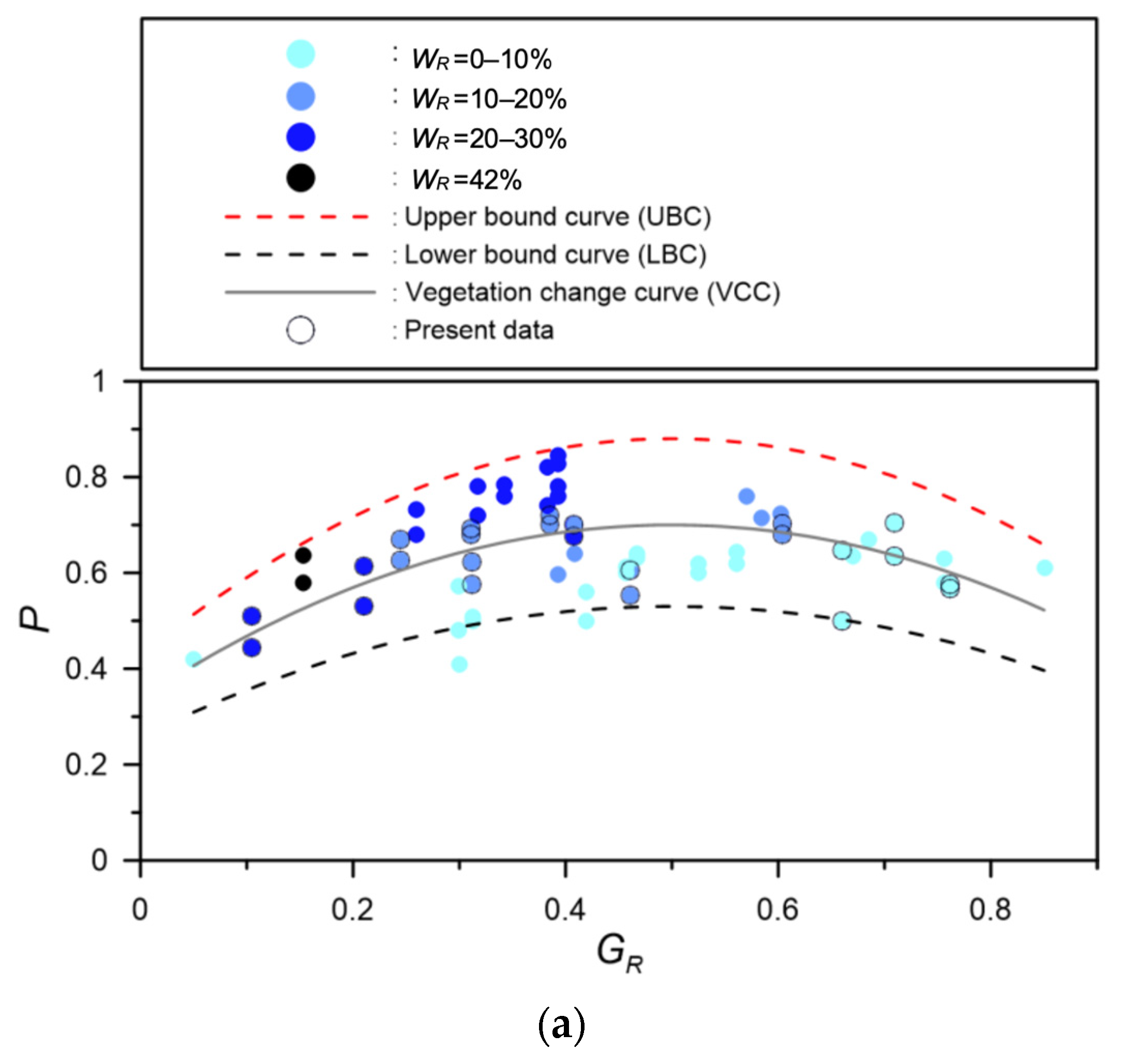
- Visual harmony H is highly correlated to visual preference P for a landscape of stream engineering in mountainous regions. The perceived curve of vegetation change (VCC) that responds to variations of visual harmony and preference owing to vegetation changes were determined. We found that 1.25 and 0.75 times of VCC can be used to describe the upper and lower bound curves for the stream landscape.
- Vegetation invasion can improve visual quality but may decrease with excess plant growth (visible greenery > 50%) without management and maintenance. Both H and P can be improved by cleaning excess vegetation in riverbeds or riverbanks. The model for the relationship between H (or P) and GR proposed herein can be used as reference for the maintenance of streams structures in mountainous regions.
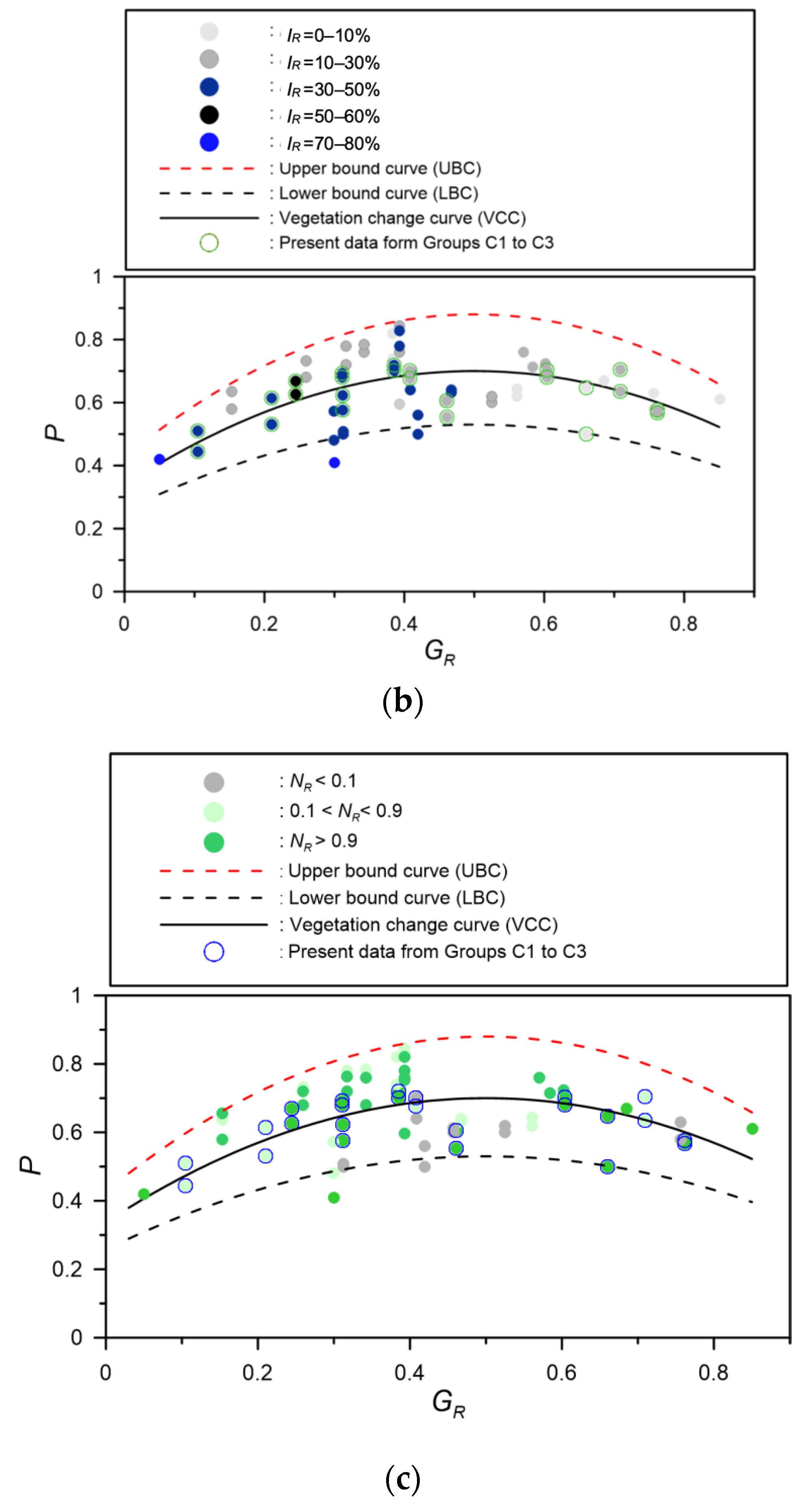
- H and P can be altered by adjusting the softscape and hardscape. Both and visible water need to be increased to improve H and P, if < 50%. Generally, < 10% is unfavorable to visual harmony and may reduce preference. Hardscape elements also have a positive effect if the visibility of engineering structures (IR) is below 30% and the proportion of natural materials on structure (NR) is over 0.9.
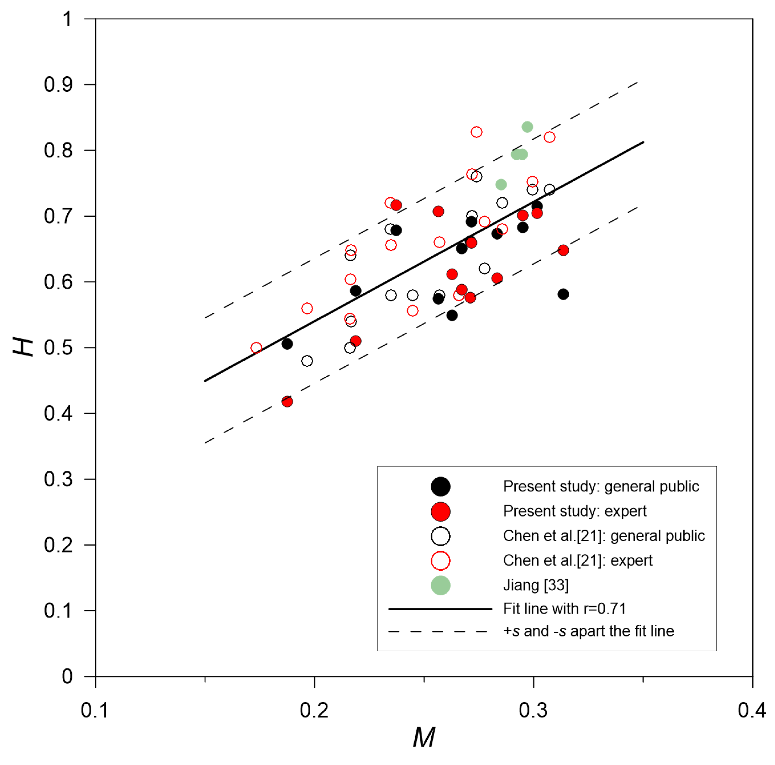
- The model of H (or P) and the combined physical indicator was developed. This model is composed of visible indicators, , , , and , that can be taken by an image. It is convenient for the designer or manager to determine a stream landscape with engineering structures, which can be preferred by the public or harmonious with the surrounding environment. Results of this study could improve the visual beauty for stream engineering and environment design.
- Images analysed in this study were limited to a landscape with engineering structures in Taiwan’s mountain streams. The model of visual harmony (or preference) was developed under the following conditions: stream width of 5 m to 20 m; stream gradient of 5–40%; an image showing a view with both sides of river visible at an accessible height; and the physical visual indicators in the ranges of 5% << 85%, < 42%, < 80%, and < 1.0. However, other factors such as color (seasonal changes in vegetation) and arrangement of landscape elements, such as water form and landform, were not included and should be explored in future studies.
Author Contributions
Funding
Data Availability Statement
Acknowledgments
Conflicts of Interest
Appendix A
References
- Wu, H.-L.; Feng, Z.-y. Ecological engineering methods for soil and water conservation in Taiwan. Ecol. Eng. 2006, 28, 333–344. [Google Scholar] [CrossRef]
- Zuo, Q.T.; Zhang, Y.; Lin, P. Index system and quantification method for human-water harmony. J. Hydraul. Eng. 2008, 39, 440–447. [Google Scholar]
- Ding, Y.; Tang, D.; Dai, H.; Wei, Y. Human-Water Harmony Index: A New Approach to Assess the Human Water Relationship. Water Resour. Manag. 2014, 28, 1061–1077. [Google Scholar] [CrossRef]
- Zuo, Q.; Li, W.; Zhao, H.; Ma, J.; Han, C.; Luo, Z. A Harmony-Based Approach for Assessing and Regulating Human-Water Relationships: A Case Study of Henan Province in China. Water 2021, 13, 32. [Google Scholar] [CrossRef]
- Zingraff-Hamed, A.; Bonnefond, M.; Bonthoux, S.; Legay, N.; Greulich, S.; Robert, A.; Rotgé, V.; Serrano, J.; Cao, Y.; Bala, R.; et al. Human–River Encounter Sites: Looking for Harmony between Humans and Nature in Cities. Sustainability 2021, 13, 2864. [Google Scholar] [CrossRef]
- Ćosić-Flajsig, G.; Vučković, I.; Karleuša, B. An Innovative Holistic Approach to an E-flow Assessment Model. Civ. Eng. J. 2020, 6, 2188–2202. [Google Scholar] [CrossRef]
- Ou, L.-C.; Luo, M.R. A colour harmony model for two-colour combinations. Color Res. Appl. 2006, 31, 191–204. [Google Scholar] [CrossRef]
- Schloss, K.B.; Palmer, S.E. Aesthetic response to color combinations: Preference, harmony, and similarity. Atten. Percept. Psychophys. 2011, 73, 551–571. [Google Scholar] [CrossRef]
- Ebigbagha, S. Achieving Harmonious Colour Relationship in Art/Design: Towards a Mathematical Model. Afr. Res. Rev. 2015, 9, 157. [Google Scholar] [CrossRef] [Green Version]
- Rahnama, M.R.; Khavari, F. Analytical Study of Color Harmony in Urban Spaces of Mashhad, Northeast Iran. Int. J. Sci. Eng. Res. 2014, 5, 756–762. [Google Scholar]
- Zhu, X.; Tan, S. Degree of Harmony of Urban Land Use and Economic Development: Case Study of Wuhan Metropolitan Area. J. Sustain. Dev. 2014, 7, 139. [Google Scholar] [CrossRef]
- Judd, D.B.; Wyszecki, G. Color in Business, Science, and Industry, 3rd ed.; John Wiley & Sons, Ltd: New York, NY, USA, 1975; Volume 42, p. 576. [Google Scholar]
- Palmer, S.E.; Schloss, K.B.; Sammartino, J. Visual Aesthetics and Human Preference. Annu. Rev. Psychol. 2013, 64, 77–107. [Google Scholar] [CrossRef] [Green Version]
- United States Forest Service. Landscape Aesthetics: A Handbook for Scenery Management; U.S. Department of Agriculture, Forest Service: Washington, DC, USA, 1995.
- Bell, S. Landscape: Pattern, Perception and Process; Routledge: London, UK, 2012. [Google Scholar]
- Tveit, M.; Ode, Å.; Fry, G. Key concepts in a framework for analysing visual landscape character. Landsc. Res. 2006, 31, 229–255. [Google Scholar] [CrossRef]
- Litton, R.B. Water and Landscape: An Aesthetic Overview of the Role of Water in the Landscape; Water Information Center: New York, NY, USA, 1974. [Google Scholar]
- Kaplan, R. Down by the Riverside: Informational Factors in Waterscape Preference; USDA Forest Service General Technical Report: Washington, DC, USA, 1977; pp. 285–289.
- Mansvelt, J.; Kuiper, J.J. Criteria for the humanity realm: Psychology and physiognomy and cultural heritage. In Checklist for Sustainable Landscape Management; Elsevier: London, UK, 1999. [Google Scholar]
- Kuiper, J. Landscape quality based upon diversity, coherence and continuity: Landscape planning at different planning-levels in the River area of The Netherlands. Landsc. Urban Plan 1998, 43, 91–104. [Google Scholar] [CrossRef]
- Chen, J.-C.; Cheng, C.-Y.; Huang, C.-L.; Chen, S.-C. Assessment of the Visual Quality of Sediment Control Structures in Mountain Streams. Water 2020, 12, 3116. [Google Scholar] [CrossRef]
- Memari, S.; Pazhouhanfar, M. Role of Kaplan’ Preference Matrix in the Assessment of Building façade, Case of Gorgan, Iran. Arman. Archit. Urban Dev. 2018, 10, 13–25. [Google Scholar]
- Junker Koehler, B.; Buchecker, M. Aesthetic Preferences Versus Ecological Objectives in River Restorations. Landsc. Urban Plan. 2008, 85, 141–154. [Google Scholar] [CrossRef]
- Stewart, W.; Larkin, K.; Orland, B.; Anderson, D. Boater preferences for beach characteristics downstream from Glen Canyon Dam, Arizona. J. Environ. Manag. 2003, 69, 201–211. [Google Scholar] [CrossRef]
- Arnberger, A.; Eder, R.; Preiner, S.; Hein, T.; Nopp-Mayr, U. Landscape Preferences of Visitors to the Danube Floodplains National Park, Vienna. Water 2021, 13, 2178. [Google Scholar] [CrossRef]
- Piégay, H.; Gregory, K.; Bondarev, V.; Chin, A.; Dahlstrom, N.; Elosegi, A.; Gregory, S.; Joshi, V.; Mutz, M.; Rinaldi, M.; et al. Public Perception as a Barrier to Introducing Wood in Rivers for Restoration Purposes. Environ. Manag. 2005, 36, 665–674. [Google Scholar] [CrossRef]
- Chin, A.; Daniels, M.D.; Urban, M.A.; Piégay, H.; Gregory, K.J.; Bigler, W.; Butt, A.Z.; Grable, J.L.; Gregory, S.V.; Lafrenz, M.; et al. Perceptions of wood in rivers and challenges for stream restoration in the United States. Env. Manag. 2008, 41, 893–903. [Google Scholar] [CrossRef] [PubMed]
- Wilson, M.I.; Robertson, L.D.; Daly, M.; Walton, S.A. Effects of visual cues on assessment of water quality. J. Environ. Psychol. 1995, 15, 53–63. [Google Scholar] [CrossRef]
- Peng, S.-H.; Han, K.-T. Assessment of Aesthetic Quality on Soil and Water Conservation Engineering Using the Scenic Beauty Estimation Method. Water 2018, 10, 407. [Google Scholar] [CrossRef] [Green Version]
- Ho, L.-C.; Chen, J.-C.; Chang, C.-Y. Changes in the visual preference after stream remediation using an image power spectrum: Stone revetment construction in the Nan-Shi-Ken stream, Taiwan. Ecol. Eng. 2014, 71, 426–431. [Google Scholar] [CrossRef]
- Kaplan, R.; Kaplan, S. The Experience of Nature: A Psychological Perspective; Cambridge University Press: New York, NY, USA, 1989; pp. 340. [Google Scholar]
- Ode, Å.; Fry, G.; Tveit, M.S.; Messager, P.; Miller, D. Indicators of perceived naturalness as drivers of landscape preference. J. Environ. Manag. 2009, 90, 375–383. [Google Scholar] [CrossRef]
- Jiang, J.-G. Visual Preference Assessment on Streams; Huafan University: New Taipei City, Taiwan, 2016. [Google Scholar]


| Location | Watershed Area (ha) | Mainstream Length (km) | Stream Width (m) | Average Riverbed Slope | Engineering Structures |
|---|---|---|---|---|---|
| Gungfunnan creek | 866 | 5.5 | 6–15 | Mainstream: 7.07%; Tributary: 15–17% | Stone revetments, stone groundsills, and submerged dam |
| Chotengkeng creek | 1320 | 8.0 | 10–20 | Mainstream: 2.7%; Tributary: 10–16% | Declined groundsill with stone lining |
| Researchers | Perceived Factors | Source of Images | Groups in Questionnaire | Rates in Questionnaire |
|---|---|---|---|---|
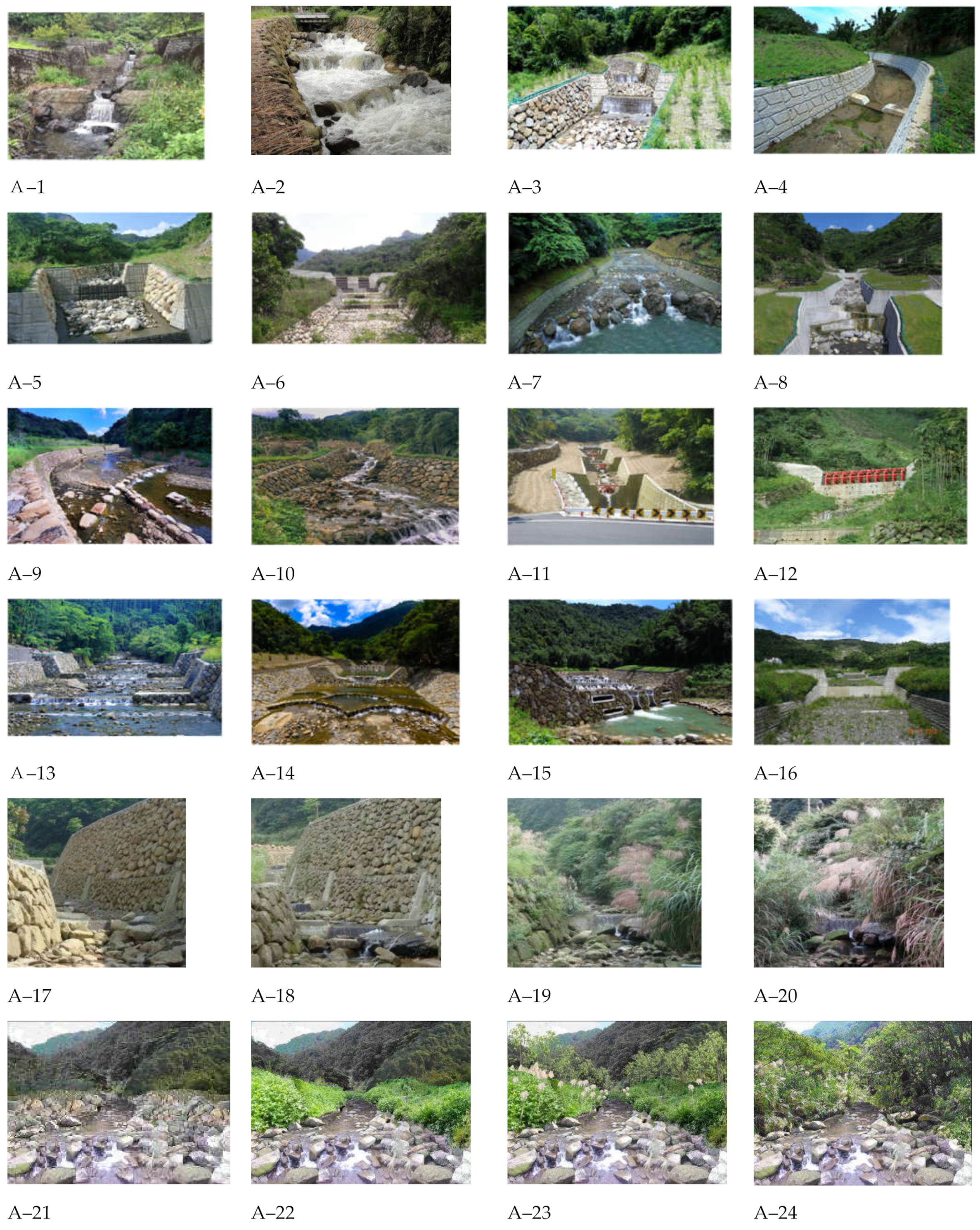
| Ho et al. [30] | Visual preference and naturalness | Field images show changes to stream landscape from vegetation invasion on stone revetments in the Nan-Shi-Ken stream, Northern Taiwan; includes four images, A–17 to A–20 as shown in Figure A1, at a fixed site at different times after the stream remediation | No specific classification | The values of visual preference and naturalness were divided into eight intervals from zero to one |
| Jiang [33] | Visual preference, naturalness, harmony, closeness, vividness, continuity, and mystery | Changes to stream landscape from vegetation invasion on riversides in Northern Taiwan; includes four images, A–21 to A–24 as shown in Figure A1, at a fixed site using image simulation | No specific classification | Five-point Likert scale from 5 (highest) to 1 (lowest); the scores are normalized (divided by 5) to 1, 0.8, 0.6, 0.4, and 0.2 in this study for comparison |
| Chen et al. [21] | Visual preference, naturalness, harmony, closeness, and vividness | Sediment control structures including revetments, grade control structures, submerged dams, and check dams constructed by the Soil and Water Conservation Bureau, Taiwan, in mountain streams; includes sixteen images, A–1 to A–16 as shown in Figure A1, collected from different sites | Expert and general public |
Publisher’s Note: MDPI stays neutral with regard to jurisdictional claims in published maps and institutional affiliations. |
© 2021 by the authors. Licensee MDPI, Basel, Switzerland. This article is an open access article distributed under the terms and conditions of the Creative Commons Attribution (CC BY) license (https://creativecommons.org/licenses/by/4.0/).
Share and Cite
Chen, J.-C.; Huang, C.-L.; Chen, S.-C.; Tfwala, S.S. Visual Harmony of Engineering Structures in a Mountain Stream. Water 2021, 13, 3324. https://doi.org/10.3390/w13233324
Chen J-C, Huang C-L, Chen S-C, Tfwala SS. Visual Harmony of Engineering Structures in a Mountain Stream. Water. 2021; 13(23):3324. https://doi.org/10.3390/w13233324
Chicago/Turabian StyleChen, Jinn-Chyi, Chia-Ling Huang, Su-Chin Chen, and Samkele S. Tfwala. 2021. "Visual Harmony of Engineering Structures in a Mountain Stream" Water 13, no. 23: 3324. https://doi.org/10.3390/w13233324
APA StyleChen, J.-C., Huang, C.-L., Chen, S.-C., & Tfwala, S. S. (2021). Visual Harmony of Engineering Structures in a Mountain Stream. Water, 13(23), 3324. https://doi.org/10.3390/w13233324