Article

Temperature Affects the Time Required to Discern the Relationship between Primary Production and Export Production in the Ocean

1
Department of Environmental Sciences, College of the Coast & Environment, Louisiana State University, Baton Rouge, LA 70803, USA
2
Department of Oceanography & Coastal Sciences, College of the Coast & Environment, Louisiana State University, Baton Rouge, LA 70803, USA
*
Author to whom correspondence should be addressed.
Water 2021, 13(21), 3085; https://doi.org/10.3390/w13213085
Submission received: 21 September 2021 / Revised: 30 October 2021 / Accepted: 2 November 2021 / Published: 3 November 2021
(This article belongs to the Section Oceans and Coastal Zones)

Abstract

:
Knowledge of the relationship between net primary production (NPP) and export production (EP) in the ocean is required to estimate how the ocean’s biological pump is likely to respond to climate change effects. Here, we show with a theoretical food web model that the relationship between NPP and EP is obscured by the following phenomena: (1) food web dynamics, which cause EP to be a weighted average of new production (NP) over a previous temperature-dependent time interval that can vary between several weeks at 25 °C to several months at 0 °C and, hence, to be much less temporally variable than NP and (2) the temperature dependence of the resiliency of the food web to perturbations, which causes the return to equilibrium to vary from roughly 50 days at 0 °C to 5–10 days at 25 °C. The implication is that the relationship between NPP and EP can be discerned at tropical and subtropical latitudes if measurements of NPP and EP are averages or climatologies over a timeframe of roughly one month. At high latitudes, however, measurements may need to be averaged over a timeframe of roughly one year because the food webs at high latitudes are very likely far from equilibrium with respect to NPP and EP much of the time, and the model can describe only the average behavior of such physically dynamic systems.

1. Introduction

The efficiency with which organic matter fixed in the euphotic zone is exported to the ocean interior is a critical determinant of the ability of the ocean to sequester carbon [1]. Quantifying that efficiency has proven to be problematic for several reasons. Station ALOHA, for example, is a site (22°45′ N, 158°00′ W) in the North Pacific Ocean of long-term studies that were initiated in 1988 to monitor and understand trends in physical and biochemical properties of the ocean at this distinctly oligotrophic location. The site is located ~100 km north of the Island of Oahu, where the water depth is 4750 m. Primary production rates in the euphotic zone estimated with 14C tracer methodology and concentrations of chl a at the surface have averaged 540 mg C m−2 d−1 and 0.28 mg m−3 since 1988 (https://hahana.soest.hawaii.edu/hot/hot-dogs/interface.html). Even in oligotrophic waters like Station ALOHA, where seasonal effects are small compared to most other parts of the ocean, the coefficient of variation of daily photosynthetic rates is 70% [2]. Hence, there is considerable temporal variability of net primary production (NPP) that can confound the interpretation of export efficiencies if rates of NPP and export production (EP) are not averaged over appropriate time scales [3,4,5]. Furthermore, the mechanisms responsible for export, collectively referred to as the biological pump, include sinking of particles, grazing by vertical migrators, and subduction of dissolved organic matter [6,7,8].The sinking of particles is a more-or-less continuous process but may also be episodic, e.g., agglomeration and sinking of phytoplankton cells following a bloom [9,10]; grazing by vertical migrators occurs on a diel time scale, and subduction of dissolved organic matter is both episodic and seasonal [11,12]. Because organic matter cannot be exported until it is first produced, and because the mechanisms responsible for exporting organic matter are not intrinsically coupled to photosynthesis, there is understandably a time lag between photosynthetic production of organic matter and its export from the euphotic zone. Photosynthesis occurs only during daylight hours, for example, whereas export production occurs during both the day and night. Any organic carbon exported from the euphotic zone at night was obviously fixed during a previous photoperiod.
The cause of the temporal delay between the production and export of organic matter is closely related to the fact that most primary production in the ocean is regenerated production, sensu Dugdale and Goering [13]. Pulses of allochthonous nutrients initially taken up by phytoplankton are therefore recycled many times before being exported. The food web responds to variations of new production in a manner analogous to the response of a low-pass electrical resistor-capacitor (RC) circuit to changes of the input voltage. In the case of an RC circuit, the lag time associated with the response of the output voltage is RC. In the case of a food web, the lag time is a function of the dynamics of the food web, which is temperature-dependent. Lag times between the production and export of organic matter may therefore tend to be long (e.g., more than one month) at high latitudes and short (e.g., less than one week) at low latitudes [5,14,15]. These time lags confound efforts to relate export production to primary production unless measurements are averaged over appropriate spatiotemporal scales [16].
In a steady state, net community production (NCP) and EP should be identical, but Estapa et al. [17] found that estimates of NCP and EP were closely correlated (r = 0.72, p = 0.04) only when data collected at 1-km intervals along eight 30–40 km-long transects across strong physical gradients in the Sargasso Sea were averaged for each transect. There was virtually no correlation in the absence of such averaging. The explanation is presumably that some degree of spatiotemporal averaging is required to discern relationships between primary production and export production. A clear correlation (r = 0.88, p = 0.00015) also emerges between NPP and EP at Station ALOHA when the NPP and EP are calculated from monthly climatologies rather than daily incubations for NPP and one-week deployments of sediment traps for EP [4,16]. In the case of Station ALOHA, the time lag between the production and export of organic matter is longer than one day but much less than one month. Bisson et al. [4] have analyzed estimates of NPP and EP averaged within 591 latitude–longitude bins (1° × 1°) at latitudes below 65° throughout the ocean. They concluded that calibrating global models of EP with field data will require “a global array of long-term flux measurement sites” and that observations be carried out “for three to seven days per month throughout the year” [4] p. 1326. Henson et al. [5] have used a food web model to carry out a theoretical analysis of this problem and concluded that the time lags between NPP and EP vary from 0–10 days “in upwelling regions and surrounding low-latitude areas (Benguela upwelling, equatorial Pacific, and Arabian Sea)” to 30–40 days at the “oligotrophic gyre edges and the Arctic” [5] p. 38.
Here, we have tested the hypothesis that a steady state food web model with adjustable parameters chosen to produce steady states with maximum resiliency to perturbations can explain observed relationships between NPP and EP when rates are averaged over appropriate spatiotemporal scales. We argue, based on comparisons between the behavior of the food web model and field data, that the time lag between the production and export of organic matter, as well as the spatiotemporal scale of field measurements required to obtain meaningful estimates of the relationship between NPP and EP, are closely related to the response of the food web model to perturbations, quantified in terms of the least negative eigenvalue of the community matrix of the model [18]. We argue that results obtained with this approach are consistent with many extant field data and that the approach can be applied to some but not all parts of the ocean where field data are sparse or lacking.

2. Food Web Model

The model is conceptually identical to the food web model described by Laws et al. [19] and is shown diagrammatically in Figure 1. Primary production is assumed to be limited by the supply of inorganic nitrogen. There are two parallel food chains: one with small phytoplankton as the first trophic level and the other with large phytoplankton as the first trophic level. The small phytoplankton are grazed by flagellates, which, in turn, are grazed by ciliates, and the dissolved organic nitrogen excreted by the small phytoplankton, flagellates, and ciliates is taken up by heterotrophic bacteria, which are preyed upon by the flagellates. The large phytoplankton and ciliates are grazed by filter feeders, which, in turn, are grazed by carnivores. The detrital organic nitrogen released by the filter feeders and carnivores is assumed to consist of particles that, along with a portion of the large phytoplankton production and dead carnivores, sinks out of the system and constitutes the export production. The mortality rate of the carnivores is assumed to be M per unit biomass per day. The flagellates are assumed to graze the small phytoplankton and bacteria in proportion to the relative biomasses of these two prey groups, and the filter feeders are likewise assumed to graze the large phytoplankton and ciliates in proportion to the relative biomasses of those two prey groups. The rate of consumption of prey by a predator is assumed to follow a relationship postulated by Steele [20]:
Fm = AmXm(Xm−1 − Pm)/Xm−1 = AmXmfm
where Am is the prey-saturated grazing rate by the predator Xm; Pm is the concentration of prey, Xm−1, at which grazing by Xm ceases, and fm is the growth rate of Xm expressed as a fraction of its prey-saturated growth rate. An equation analogous to Equation (1) applies to the uptake of inorganic nitrogen by phytoplankton. Of the prey nitrogen consumed by a predator, a fraction r is respired, a fraction s is excreted, and a fraction q is incorporated into biomass. Therefore r + s + q = 1. For phytoplankton, a fraction s of the inorganic nitrogen taken up is excreted as organic nitrogen, and a fraction q is incorporated into phytoplankton biomass. Photosynthetic rates are therefore understood to be net rather than gross photosynthetic rates, and for phytoplankton, q + s = 1. The following 10 equations then describe the dynamics of the food web:
dX1/dt = L − (1 − r2L)F2L − (1 − r2s)F2s + r3F3 + r4F4 + r5F5 + r6F6 + rBFB
dX2S/dt = q2SF2S − F3X2S/(X2S + XB)
dX2L/dt = q2LF2L − F5X2L/(X2L + X4)
dX3/dt = q3F3 − F4
dX4/dt = q4F4 − F5X4/(X2L + X4)
dX5/dt = q5F5 − F6
dX6/dt = q6F6 − MX6
dDOM/dt = S2SF2S + S3F3 + S4F4 − FB
dPOM/dt = S2LF2L + S5F5 + S6F6 − FB + MX6 − D⋅POM
dXB/dt = qBFB − F3XB/(X2S + XB)
The assumption that the ciliates graze XB and X2S in proportion to XB/(X2S + XB) and X2S/(X2S + XB), respectively (Equations (3) and (11)), requires that the growth rates of the XB and X2S be identical in the steady state. This conclusion follows from the fact that the right-hand sides of Equations (3) and (11) can be written as [μ2S − F3/(XB + X2S)]X2S and [μB − F3/(XB + X2S)]XB, respectively, where μ2S and μB are the growth rates of X2S and XB, respectively. This condition then requires that fBqBAB = f2Sq2SA2S. Likewise, Equations (4) and (6), combined with the assumption of steady state, require that the growth rates of the large phytoplankton and ciliates be identical, i.e., f4q4A4 = f2Lq2LA2L. The steady state assumption further implies that M = q6A6f6 and that L = D⋅POM.
Table 1 lists the parameters in the model that were either assumed to be constant or were explicit functions of temperature. The temperature dependence of the parameters is especially important to the behavior of the model. The temperature dependence of the nutrient-saturated phytoplankton growth rates was taken from Eppley [21]. The model assumes that under nutrient-saturated conditions, both the small and large phytoplankton are capable of growing at an average rate of 1.2 d−1 within the euphotic zone at a temperature of 25 °C. This assumption is consistent with growth rates reported from field work in the subtropical gyres and equatorial Pacific [22,23,24,25]. The substrate-saturated heterotrophic bacterial growth rates were assumed to follow the same pattern as the nutrient-saturated phytoplankton growth rates. This assumption was based in part on heterotrophic bacterial growth rates reported from field studies, which differ little from phytoplankton growth rates reported under similar conditions [26]. Reported Q10 values for heterotrophic bacterial growth rates lie in the range of ~2–4 [26,27] and are positively correlated with chlorophyll a (chl a) concentrations [26]. The assumed Q10 for heterotrophic bacterial growth rates is 1.9 and gives growth rates of 0.25 d−1 at 0 °C, comparable to values reported from estuarine and coastal habitats at that temperature [26]. The maximum growth rates of the flagellates and ciliates was assumed to be identical to that of copepods [28]. The maximum ingestion rates of the filter feeders and carnivores were assumed to be 0.5 d−1 at 25 °C. This assumption gives maximum growth rates for the filter feeders and carnivores of 0.15 and 0.174 d−1, within the range of values summarized from physiological rates measurements on copepods (0.14–0.39 d−1) by Huntley and Lopez [28] at 25 °C. The temperature dependence of these rates was taken from Huntley and Lopez [28].
The values of P2S and P2L were set to 7.5 and 75 nM, respectively, based on the studies of Caperon and Meyer [29] and Sunda and Hardison [30]. PB was assumed to be numerically identical to P2S.
In the steady state, new production and export production are identical, and we have referred to the ratio of new production to NPP (f ratio: [31]) or export production to NPP (e ratio: [32,33]) as the ef ratio, in accord with [19]. With some algebra, it is straightforward to show that the ef ratio is a maximum (efmax) when all primary production is routed through the large phytoplankton, and the ef ratio is a minimum (efmin) when all primary production is routed through the small phytoplankton. These maximum and minimum ef ratios are s2L + q2L·[s5 + q5·(s6 + q6)] and (q2S + qB·s2S)·q4·q3·[s5 + q5·(s6 + q6)]/[1 − qB·(s3 + s4·q3)], respectively. Given the values of the parameters in Table 1, efmax and efmin are 0.685 and 0.128, respectively.
We assumed that the system adjusted to the external loading rate L (i.e., new production) in a manner that produced a stable steady state, as defined by May [18]. May’s definition of stability implies that the system is stable to small perturbations of the Xm from their equilibrium values. This is a reasonable requirement, because there is little point in discussing the characteristics of a steady state if the steady state is not stable to small perturbations, and in the case of this study, the food webs of interest are indeed subject to perturbations. To obtain a unique solution to the equations, we further required that the steady state solution be more stable to small perturbations than any other steady state solution. This assumption is arbitrary, and there is no a priori reason to believe that pelagic ecosystems evolve toward a condition of maximum stability. Mathematically, a steady state is stable to small perturbations if the real parts of all the eigenvalues of its community matrix are negative [18]. The community matrix for Equations (2)–(11) is a 10 × 10 matrix consisting of the partial derivatives of the right-hand sides of Equations (2)–(11) with respect to the Xm, evaluated at the equilibrium point. For example, the element in the 1st row and 2nd column of the community matrix is the partial derivative of Equation (2) with respect to the second state variable, X2S. Requiring that the system has maximum stability implies that the least negative eigenvalue associated with a given steady state be more negative than the least negative eigenvalue of any other steady state.
The steady state food web with maximum resiliency was determined at a specified temperature and rate of net NPP (mg N m−3 d−1) within the euphotic zone. The combination of the values of the ef ratio and the dimensionless parameters f2L, f3, f5, and f6 were then selected to produce a steady state with maximum stability. The parameters f2L, f3, f5, and f6 must lie in the interval 0–1, and of course, the ef ratio must lie between efmin and efmax.
The sum of F2S and F2L equals NPP, and with a little algebra, it is straightforward to show that
F2S = NPP(efmax − ef)/(efmax − efmin)
F2L = NPP(ef − efmin)/(efmax − efmin)
It is then straightforward to show that
F3 = F2S(q2S + qBS2S)/[1 − qB(S3 + S4q3)]
F4 = q3F3
F5 = q2LF2L + q4F4
F6 = q5F5
FB = S2SF2S + S3F3 + S4F4
If values are now assigned to the dimensionless parameters f2L, f3, f5, and f6 in the interval 0–1, it follows that
f4 = q2LA2Lf2L/(q4A4)
f2S = 1 − (1 − f2L)P2S/P2L
fB = q2SA2Sf2S/(qBAB)
Then
X1 = p2S/(1 − f2S)
DOM = PB/(1 − fB)
X2S = F2S/(A2Sf2S)
X2L = F2L/(A2Lf2L)
X3 = F3/(A3f3)
X4 = F4/(A4f4)
X5 = F5/(A5f5)
X6 = F6/(A6f6)
XB = FB/(ABfB)
and
Pm = (1 − fm)Xm −1, for m = 3−6
After determining the steady state values of the variables in the model, the partial derivatives of the right-hand sides of Equations (2)–(11) with respect to X1, X2S, X2L, X3, X4, X5, X6, XB, DOM, and POM were calculated to set up the community matrix [18]. The accuracy of the partial derivatives was checked by finite differencing. The combination of the ef ratio and f2L, f3, f5, and f6 that produced a steady state with maximum resilience was then determined for different combinations of temperature and NPP. Temperatures were varied between −1.8 and 30 °C; NPP was varied in a geometric series between 0.5 and 1024 mg C m−3 d−1. NPP in terms of carbon was converted to a nitrogen basis by assuming a C:N ratio of 5.68 g C g−1 N [34].

3. Results

3.1. Steady State Behavior

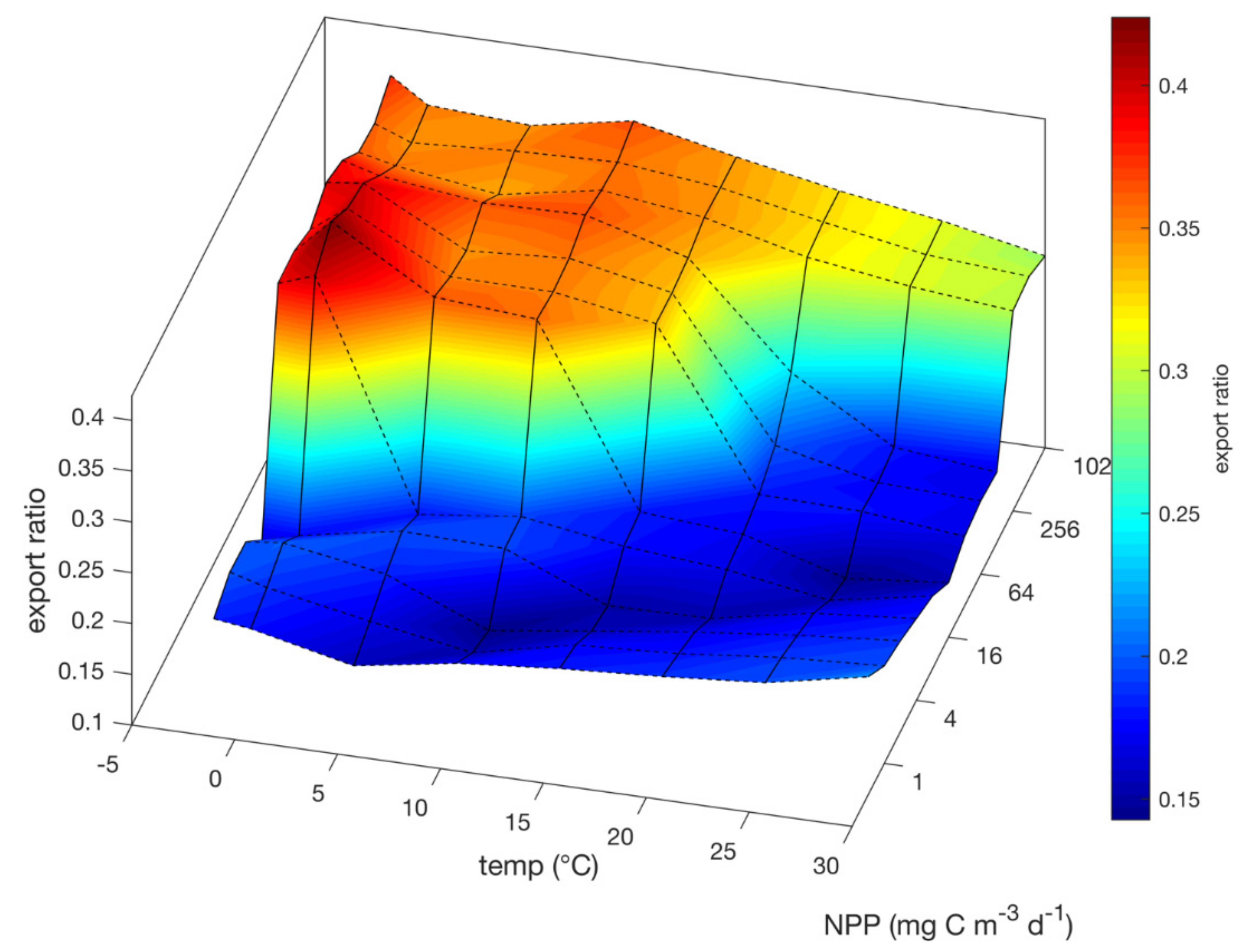
The steady state ef ratios that were associated with maximum resiliency to perturbations are shown in Figure 2 as a function of temperature and NPP. The ef ratios transitioned from low values (0.15–0.20) to high values (0.30–0.45) along a curve from low temperatures and low NPP (0 °C and <4 mg Cm−3 d−1, respectively) to high temperatures and high NPP (30 °C and >256 mg Cm−3 d−1, respectively). The low ef ratios were associated with most NPP being accounted for by small phytoplankton to roughly equal percentages of NPP being accounted for by small and large phytoplankton.
To compare the predictions of the model with field observations, we chose the dataset analyzed by Dunne et al. [35], which includes 122 estimates of NPP and EP at latitudes ranging from 1° to 82° and NPP rates from 3.75 to 641 mg C m−2 d−1. Estimates of EP came from sediment trap studies [36] or 234Th methodology [37]. We binned the data into ef intervals of 0.05 and plotted the ef ratios estimated with the model to the ratios reported by Dunne et al. [35] (Figure 3). The model appears to do a good job of predicting the ef ratios over the range of ratios from 0.15 to 0.45.
Studies at the Hawaiian Ocean Time-series (HOT) site have provided estimates of NPP and EP (sediment traps) on a monthly basis since October 1988 at 22°45′ N, 158°00′ W. Estimates of NPP have been made from bottle incubations at depths of 5, 25, 45, 75, 100, 125, and 150 m. Because the mixed layer at HOT averages 60 m, we estimated NPP and concentrations of chl a from the surface to 75 m, the shallowest depth below the depth of the mixed layer where incubations have been carried out. We estimated EP at 75 m, based on the relationship between the export flux of organic carbon and depth at HOT reported by Grabowski et al. [38]. Estimates of phytoplankton C/chl a ratios in the upper 45 m of the water column were taken from Christian and Karl [39]. Table 2 summarizes the observed and predicted results.

3.2. Time Lags

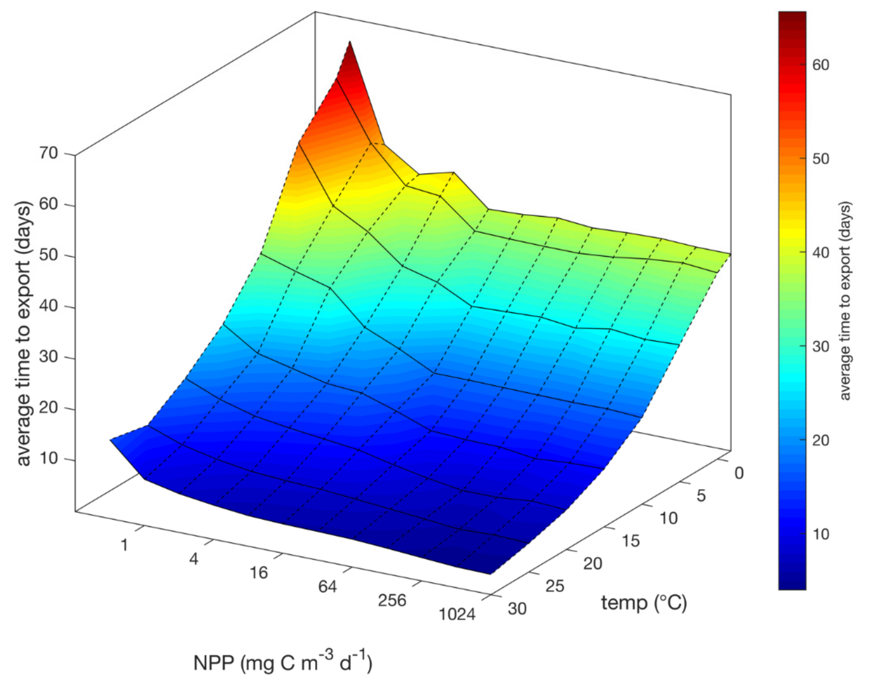
The average time required for recently fixed organic matter to be exported was negatively correlated with temperature and with NPP (Figure 4). At low temperatures and low NPP, the average time between production and export could be as long as 50–60 days, and at high temperatures and high NPP, it could be as short as 4–5 days.
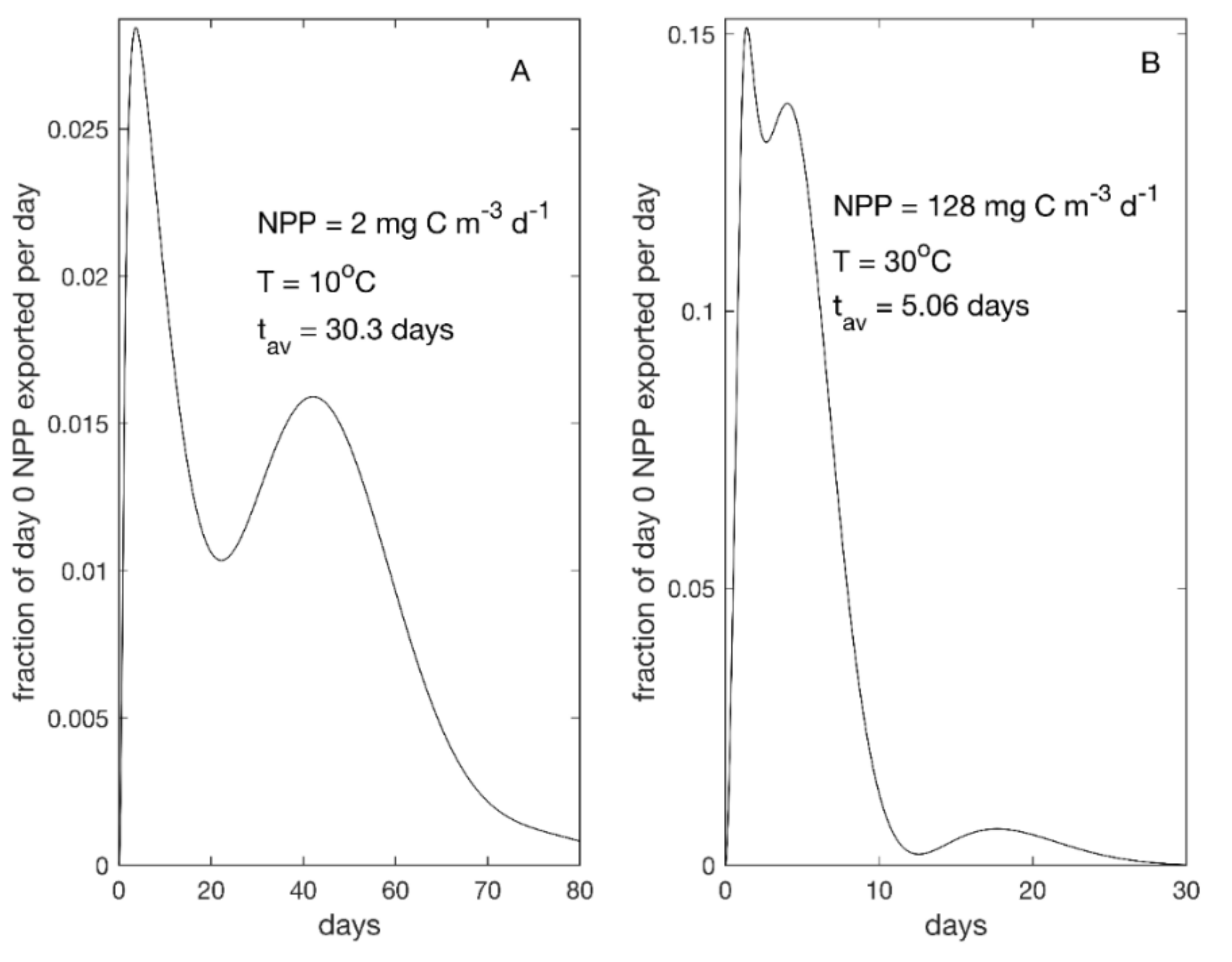
A closer examination of the relationship between new production and export production proved revealing. Although there was certainly a delay between new production and export production, the latter was not exported in a one-day pulse that occurred a fixed number of days after the associated new production. Instead, the exported production associated with new production on a given day was exported over a timeframe of many days and was characterized by two prominent pulses, the first associated with passage through the large phytoplankton food chain and the second with passage through the small phytoplankton food chain (Figure 5). This was true for both the low temperature (10 °C) and low NPP (2 mg C m−2 d−1) scenario and the high temperature (30 °C) and high NPP (256 mg Cm−3 d−1) scenario. Even when the average delay between new and export production was as short as 5 days (Figure 5B), no more than 15% of the associated new production was exported on any given day. When the average time lag was as long as 30 days (Figure 5A), the peak of export production was less than 3% of the associated new production.

3.3. Resiliency and Response to Perturbations

The resiliencies of the most stable steady state model food webs were strongly dependent on temperature and relatively weakly dependent on NPP (Figure 6). At high temperatures and high NPP, the rate of return to equilibrium after a perturbation was as rapid as 0.4 d−1, but at low temperatures and low NPP, it was as slow as 0.015 d−1.
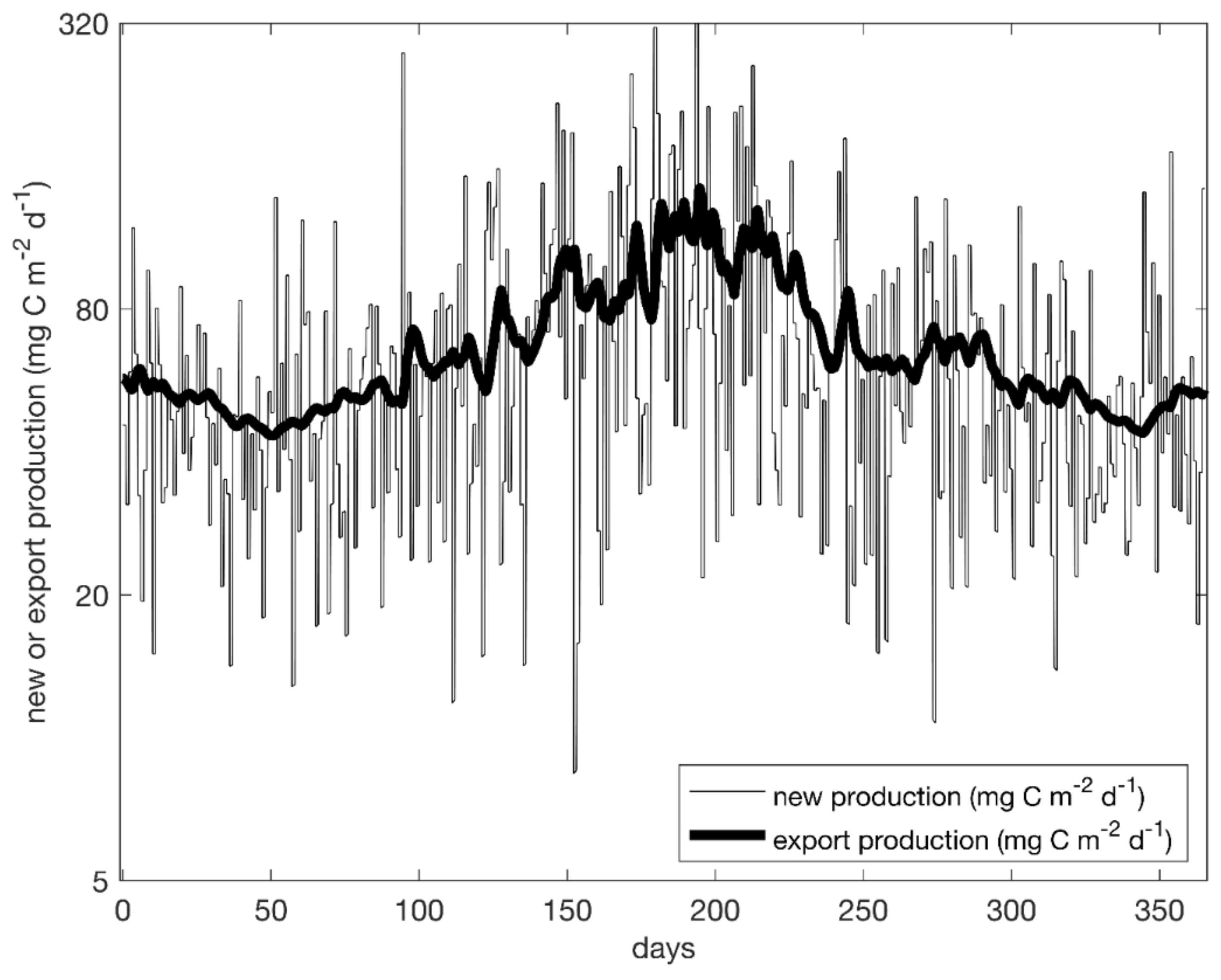
Barone et al. [2] reported that photosynthetic rates at Station ALOHA vary from day to day by 16–20%. The monthly average photosynthetic rates at Station ALOHA are available (https://hahana.soest.hawaii.edu/hot/hot-dogs/interface.html) from the web site of the Hawaii Ocean Time-series (HOT). We fitted a sinusoidal function with a period of one year to the monthly average data and estimated the average NPP and temperature in the mixed layer (60 m) from the profiles of NPP and temperature versus depth at the same web site. The average NPP and temperature were 5.92 mg C m−3 d−1 and 24.6 °C, respectively. The ef ratio at that temperature and NPP was estimated from Figure 2 to be 0.16. We assumed that the expected value of NPP varied in a sinusoidal manner with a period of one year, consistent with the monthly average NPP at Station ALOHA. We assumed that NP varied from day to day in a manner similar to NPP and used a lognormal random number generator that produced an 18% day-to-day coefficient of variation (CV) of NP. We then used a fourth-order Runge–Kutta numerical integration scheme to follow the EP predicted by the food web model over a period of one year. Figure 7 shows the results of the simulation. The CV of daily NP over the one-year simulation was 72.7%, which is very similar to the CV of 70% for NPP reported by Barone et al. [2]. The CV of the simulated EP was 32.5%, which is similar to the CV of 35% for the export production estimated from sediment traps at a depth of 150 m (HOT website). The simulated NP was clearly much more variable than the simulated EP, but the two were very similar when averaged over monthly time intervals (Figure 8, r = 0.95). The correlation in Figure 8 is very similar to the correlation between measured NPP and EP (r = 0.88, p = 0.00015) when both measurements are monthly climatologies [16].

4. Discussion

4.1. Sources of Error and Caveats

The agreement between the steady state predictions of the model and average field data is reassuring (Figure 3 and Table 2), but there are numerous sources of error in both the model and field data, and the agreement may to some extent be fortuitous, i.e., the model may have been right for the wrong reasons. First, the model contained five dimensionless, adjustable parameters, four of which could vary between 0 and 1 (f2L, f3, f5, and f6), and the fifth of which, the ef ratio, could vary between efmin (0.128) and efmax (0.685). Values were assigned to these five parameters to produce a steady state solution with maximum resilience to perturbations. It seems logical that natural systems would evolve in a way that makes them resilient to perturbations [18], and the five adjustable parameters in the case of the model food web (Equations (2)–(11)) were chosen to produce a steady state with maximum resiliency, rather than to give a good fit to field data. The assumption of maximum resiliency is arbitrary, and it is noteworthy that a model with adjustable parameters chosen to maximize resiliency to perturbations gives a good description of field data (Figure 3 and Table 2).
The food web was assumed to be nitrogen limited, and based on the work of Goldman et al. [40], it assumes that marine bacteria convert 100% of the nitrogen they take up into biomass. This assumption is clearly inappropriate for carbon. The growth efficiencies with respect to carbon of heterotrophic marine bacteria in nature have been estimated to lie somewhere between a low of 5–10% [41,42] and a high of 20–35% [43,44,45,46]. The review of heterotrophic bacterial growth efficiencies by del Giorgio and Cole [47] indicated that the efficiency with which bacteria growing on organic matter derived from phytoplankton or fecal material convert carbon into biomass is about 15%. Had we assumed a qB of 0.15 instead of 1.0, efmax would have been unchanged, but efmin would have been reduced from 0.128 to 0.054. Forty-two of the 122 export ratios in the summary by Dunne et al. [35] lie between 0.128 and 0.054. The value of qB could be varied in a systematic way to give a better fit to the experimental data, but some of the low export ratios reported from field work may reflect inconsistencies between the assumptions of the model and the way the data were collected.
The food web model envisions a well-mixed system and therefore implicitly assumes that the depth of the euphotic zone equals the depth of the mixed layer. The modeled export production thus represents the export from that well-mixed system, i.e., the export from just below the depth of the mixed layer. In the summary by Dunne et al. [35], the average depth of the euphotic zone is 61 m. Sediment traps are deployed below the mixed layer depth to avoid, insofar as possible, artifacts, such as resuspension, that would be caused by physical disturbances. In the case of 234Th work, samples of particles used to estimate 234Th/carbon ratios are routinely collected well below the mixed layer depth to ensure that the particles are representative of sinking particulate matter [48]. Estimates of export production from field work are therefore likely to be smaller than the rates of export production simulated by the food web model. At Station ALOHA, for example, estimates of export production are routinely reported based on sediment traps deployed at a depth of 150 m, which is the approximate depth of the euphotic zone at that site [49] and is 90 m below the average depth of the mixed layer. The ratio of the organic carbon fluxes into sediment traps at Station ALOHA [38] to the associated photosynthetic rates give export ratios of 0.055, 0.068, and 0.089 at depths of 150, 125, and 100 m, respectively (vertical profiles dropdown menu at https://hahana.soest.hawaii.edu/hot/hot_jgofs.html). Photosynthetic rates in the upper 75 m of the water column account for 79% of the NPP at Station ALOHA (vertical profiles dropdown menu at https://hahana.soest.hawaii.edu/hot/hot_jgofs.html), and the export of organic carbon at that depth, estimated from Grabowski et al. [38], gives an export ratio of 0.13 (Table 2). The comparisons of field results with the predictions of the model are clearly confounded by the fact that the assumptions of the model (a well-mixed system and flux estimates at the base of the mixed layer) are inconsistent with export fluxes estimated in the field at depths below the mixed layer depth.
Comparisons between the model and field data should also take into consideration the uncertainties associated with the field data. In the case of export production estimated with the 234Th method [50], there are uncertainties associated with the ratio of organic carbon to 234Th in sinking particles, and for sediment traps, there are several issues related to trap design that have been summarized by Buesseler [50]. Bisson et al. [4] p. 1319 concluded that these errors can result in uncertainties of export fluxes of at least ± 30% “and can be much larger”.

4.2. The Relationship between NPP and EP

Estimates of the organic matter exported from surface waters via sinking particles have not always revealed a significant correlation between EP via sinking particles and NPP [51,52], and some recent analyses of field data have likewise revealed no relationship between EP and NPP [53]. The food web model (Figure 1) provides a logical explanation for the lack of correlation between estimates of NPP and EP when averaging is not carried out over a timeframe that is long compared to the lag between NPP and EP. However, the time lag associated with the dynamics of the food web is by no means the only mechanism that can confound the relationship between NPP and EP. The absence of any correlation when comparisons are made across wide climatic, temporal, and spatial scales could reflect a variety of processes, including spatial decoupling [17], differences in mineral ballasting [54], changes in the physiological status of the phytoplankton community [55], the flocculation and sinking of particles (including phytoplankton cells), en masse [56,57], differences in grazer communities [58,59], differences in the species composition of the phytoplankton community [55,60], changes in the lability of sinking particles with depth [38], as well as spatiotemporal offsets between the production and export of organic matter and the fact that the food web is not in a steady state [5,14,15,16].
The model predicts export production that varies slowly and over a much smaller range than new production (Figure 8). However, long-term sediment trap studies by Ducklow et al. [61] to the west of the Antarctic Peninsula (64°30′ S, 66°00′ W), where there is a late spring-summer diatom bloom and moderately high NPP in December–February, have revealed intervals of peak export production that last an average of 106 days but account for 85% of annual EP. At Station M (34°50′ N, 123°00′ W), which is located in the California Current System at a site where the water column is 4 km deep, 30 ± 10% of the annual flux of particulate organic carbon (POC) to a depth of 3400 m arrives in episodic pulses 0–70 days after satellite-based estimates of peaks in export fluxes [9]. At the same station, Preston et al. [10] have reported an episodic flux of POC in June of 2017 that accounted for 44% of the POC flux at a depth of ~3900 m during their nine-month study. The average rate of primary production at Station M, estimated via satellites, is 553 mg C m−2 d−1, very similar to the analogous rate at Station ALOHA, but the average concentration of chl a at the surface, 0.6 mg m−3, is about twice the concentration at Station ALOHA.
These observations make it clear that EP can undergo wide temporal variations in some parts of the ocean. However, the agreement between the modeled ef ratios and the export ratios summarized by Dunne et al. [35] (Figure 3) and the fact that the CVs of EP and NPP at Station ALOHA are 35% and 70%, respectively, suggest that the food web model predictions are reasonable and that, at least for sites like Station ALOHA, the CV may be much smaller for EP than for NPP.

4.3. Effects of Lateral Currents

Most field studies of the relationships between NPP and EP implicitly assume that lateral current movements do not confound the downward flux of organic matter. Siegel and Deuser [62] have pointed out that the typical sinking rates of particles, 50–200 m d−1, are roughly an order of magnitude slower than the typical speeds of horizontal currents. As a result, “sinking oceanic particles approach sediment traps at near-horizontal angles” [62] p. 1532, and the effective collection area of a sediment trap at a depth of 100 m can easily be in the order of 10 km2. The Rossby radius of deformation, a typical horizontal scale of mesoscale eddies, is about 50 km near Hawaii, for example, and horizontal velocities are by no means uniform. The area of the collection funnel for particles that fall into sediment traps at a depth of 150 m can therefore be greater than 50 km2 [63].Unless photosynthetic rates are uniform within the statistical funnel that defines the volume of water sampled by a sediment trap, physical processes will confound the relationship between NPP and EP.

4.4. Time Lags and Temperature

The time lags between production and export simulated by the model food web (Figure 4) are very much a function of the assumed temperature dependence of the community of heterotrophs in the model. Thirty percent of the production of large phytoplankton is assumed to be directly exported (S2L in Equation (10)), but all other phytoplankton production is passed through the food web of heterotrophic organisms, and much of it is respired and recycled before it is exported. The assumed temperature dependence of heterotrophic processes corresponds to a Q10 of 2.7, with the exception of the bacteria, for which the Q10 is 1.9. This temperature dependence of heterotrophic processes accounts for the dramatic increase of the time lags between production and export at low temperatures (Figure 4), and the recycling that occurs within the food web explains why the production from a single day is exported in small increments over a timeframe of many days (Figure 5). The latter behavior provides a logical explanation for the results of the 11 iron fertilization experiments summarized by Boyd et al. [64], only five of which resulted in a detectable increase of export production. The dynamics of the model suggest that the food web behaves much like the capacitor in an electrical circuit. Abrupt increases of new production are turned over many times before being exported, as noted by Forest et al. [65]. The result is that the pulse of export production occurs over a longer timeframe than the pulse of new production, and the peak of export production is much attenuated compared to the peak of new production (Figure 7). The dynamics of the food web thus account, at least in part, for the poor correlation that is typically observed between new production and export production when the two are not averaged over sufficiently large spatiotemporal scales. Our simulation of results at Station ALOHA (Figure 7 and Figure 8), however, suggests that at temperatures of ~25 °C, averaging over time intervals of roughly one month can overcome the artifacts associated with time lags, a conclusion consistent with previous analyses [4,5,16].

4.5. Steady State or Not

Several problems arise at high latitudes, where temperatures may lie in the range −1.8 to 10 °C. First, the time lags between production and export may easily be one month or more. Second, the food web is much less resilient to perturbations than it is at warmer temperatures (Figure 6), and environmental seasonality is much greater than it is at lower latitudes. The food web is therefore likely to be far from equilibrium at the current temperature, irradiance, and nutrient concentrations. The result can be dramatic pulses of production and export of organic matter [61] that are unrelated to the predictions of a steady state model. In such cases, we concur with the recommendation of Bisson et al. [4] p. 1326 that observations be carried out “for three to seven days per month throughout the year” to obtain accurate estimates of the relationship between NPP and EP. It is likewise clear that the food web model does not apply to places like Station M, where large, episodic pulses of EP have been documented [9]. However, the good agreement between the predictions of the food web model and the data summarized by Dunne et al. [35], which includes 122 estimates of NPP and EP at latitudes ranging from 1° to 82° (Figure 3), suggests that the steady state assumption leads to reasonable predictions of ef ratios in many parts of the ocean.

4.6. Response to Perturbations

The response of export production to abrupt perturbations of new production (Figure 7) illustrates an issue pointed out by Forest et al. [65] pp. 740–741: “hence we must take into account the time needed for phytoplankton cells to grow and aggregate, as well as the various trophodynamic processes that may turnover the biomass derived from PP [primary production] many times before being vertically exported… our relationships confirm the existence of an efficient retention system and a high degree of recycling within the upper water column.” Our simulated results indicate that when there are abrupt increases of new production on a day-to-day basis, there is a time lag between the peak of new production and the peak of export production that is negatively correlated with temperature and may range from roughly 5 to 50 days. This pattern is consistent with the modeling study of Henson et al. [5], the mesocosm studies of Stange et al. [15], and the field studies of Michaels and Knap [52], Benitez-Nelson et al. [14], and Alkire et al. [66].
Abrupt increases of new production are turned over many times before being exported, as noted by Forest et al. [65]. The result is that the pulse of export production occurs over a longer timeframe than the pulse of new production, and the peak of export production is much more attenuated compared to the peak of new production (Figure 7). The dynamics of the food web thus account, at least in part, for the poor correlation that is typically observed between new production and export production when the two are not averaged over sufficiently large spatiotemporal scales (e.g., Figure 7 versus Figure 8).
Because most primary production in the ocean is associated with allochthonous rather than autochthonous nutrients [19], most new production is initially recycled rather than exported [65]. The result is that variations of NP are averaged over a temperature-dependent timeframe that can vary from roughly several weeks to several months (Figure 5). This integration causes rates of EP to be relatively constant compared to rates of NPP and, hence, to be uncorrelated with NPP [5,14,15,16] when estimates of NPP come from measurements that cover a timeframe of no more than a few days. At 25 °C, it is possible to discern the relationship between NPP and EP when estimates are based on monthly climatologies [16] because the recovery time of the food web from perturbations at 25 °C (5–15 days) is short compared to one month. At Station ALOHA, where temperatures in the euphotic zone average 24.2 °C, the dynamics of the food web are such that an annual cycle of NP that varies by ± 30% still results in a good correlation between NP and EP (Figure 6), but the time lag of ~13 days between NP and EP explains why there is virtually no correlation between photosynthetic rates and EP, when the former are based on 24-h measurements [5,14,15,52].
The dynamics of the model are also consistent with observations of the responses of large and small phytoplankton biomass to pulses of new production. In all cases the small and large phytoplankton are growing at ~90% and ~10% of their nutrient-saturated growth rates in the steady state associated with maximum resiliency to perturbations. A pulse of nutrients, therefore, has little effect on the growth rates of the small phytoplankton but can increase the growth rates of the large phytoplankton by roughly a factor of 10. The response of the model to a pulse of nutrients is, therefore, consistent with the observation, for example, that the abundance of picoplankton is virtually unchanged during El Niño and normal upwelling periods in the equatorial Pacific, but diatoms and other large phytoplankton increase substantially during normal upwelling events (Bidigare and Ondrusek, 1996; Landry et al., 1996) and in response to iron fertilization (Landry et al., 1997). The model assumes (Table 1) that the flagellates (X3) have a much higher maximum growth rate than the filter feeders (X5), and under conditions of maximum resilience, the flagellates are never growing at more than about 20% of their maximum growth rate, whereas the filter feeders may be growing at 80% of their maximum growth rate. Thus, the flagellates can rapidly respond to an increase of small phytoplankton production by immediately increasing their grazing rates and thereby holding the small phytoplankton in check, whereas the filter feeders must rely more on increasing their biomass, which takes time.

5. Conclusions and Implications

The food web model (Figure 1) seems to do a good job of explaining the relationship between NPP and EP in many parts of the ocean. The fact that most NPP is autochthonous rather than allochthonous means that an abrupt increase of NP is recycled many times before being exported, and as a result, the associated change of EP lags the change of NP and appears as a relatively low-amplitude, temporally broad peak. This scenario can account for the temporal dynamics of EP in parts of the ocean where the food web is in approximate equilibrium (Figure 7). It does not account for the dynamics of EP in parts of the ocean where the food web is likely far from equilibrium because the dynamics of physical processes that control the supply of nutrients and light are much faster than the temperature-constrained rates of biological processes. In the former case, it appears that averaging NPP and EP over timeframes of roughly one month should make it possible to discern the relationship between NPP and EP [16] (Figure 8). The slower dynamics of high-latitude food webs and the much longer time lags between production and export [5] at colder temperatures suggest that longer averaging times will be necessary to discern relationships between NPP and EP in those cases. Because photosynthetic rates at high latitudes are highly seasonal, it seems reasonable to conclude that high-latitude pelagic food webs are typically far from equilibrium [66,67]. Discerning the relationship between NPP and EP in such systems may require averaging over an annual cycle [4].
Methods that could be used to obtain estimates of annual new and export production include oxygen budgets in surface waters [68,69], surface water carbon budgets constrained by measurements of the δ13C of dissolved inorganic carbon [70,71], and autonomous observations made from Argo floats and gliders. Estimates of NPP can be made from measurements of temperature and chl a fluorescence by Argo floats [72,73,74] in a manner similar to the way that NPP is estimated on the basis of satellite-based estimates of surface temperature and chl a [75], and export production can be estimated throughout the year based on the sinking particles collected in sediment traps [61]. Export production can also be estimated from depth-integrated estimates of subsurface oxygen utilization rates [76] on the assumption that the respiration is balanced by EP. In addition to being able to provide estimates of NPP and EP over annual timeframes, oxygen-based methods have the advantage of being able to account for all processes that export organic matter to the interior of the ocean and to integrate rates over spatial scales in the order of 102–103 km. The use of these methods at high latitudes will be needed to test predictions of the response of the ocean’s biological pump to climate change [77].
Although use of such methods may provide reliable empirical data that can be used to relate NPP to EP, there will remain the need for a theoretical understanding of those relationships that could be used to predict, for example, how carbon cycling and export production will change in response to global warming. Simple food web models (Figure 1) are inappropriate for describing the behavior of such physically dynamic systems. An analogy might be made to the hierarchy of quantum mechanics, statistical mechanics, and classical mechanics in physics. Quantum mechanics is not used to describe a ball rolling down an inclined plane. Theoretical tools must be chosen that are appropriate to the task. Theoretical understanding of the behavior of these physically dynamic systems remains a challenge for future work.

Supplementary Materials

The following are available online at https://www.mdpi.com/article/10.3390/w13213085/s1: values of ef, f2L, f3, f5, and f6 that produce a steady state with maximum resilience as function of temperature and NPP; Matlab computer program that can be used to find the values of ef, f2L, f3, f5, and f6 that produce a steady state with maximum resilience at any temperature and NPP.

Author Contributions

E.L. carried out the calculations and wrote the first draft of the manuscript. K.M. reviewed and revised the first draft of the manuscript to produce the final version of the manuscript. All authors have read and agreed to the published version of the manuscript.

Funding

This research was funded by National Science Foundation, USA, with grants OCE 1536581 to EAL and OCE 1756788 to KM.

Institutional Review Board Statement

Not applicable.

Informed Consent Statement

Not applicable.

Data Availability Statement

The data presented in this study are openly available online at Supplementary Materials.

Acknowledgments

We dedicate this manuscript to the memory of John Steele.

Conflicts of Interest

The authors declare no conflict of interest.

References

  1. Sarmiento, J.L.; Bender, M. Carbon biogeochemistry and climate change. Photosynth. Res. 1994, 39, 209–234. [Google Scholar] [CrossRef] [PubMed]
  2. Barone, B.; Nicholson, D.; Ferron, S.; Firing, E.; Karl, D.M. The estimation of gross oxygen production and community respiration from autonomous time-series measurements in the oligotrophic ocean. Limnol. Oceanogr. Methods 2019, 17, 650–664. [Google Scholar] [CrossRef] [Green Version]
  3. Karl, D.M.; Laws, E.A.; Morris, P.; Williams, P.J.L.; Emerson, S. Metabolic balance of the open sea. Nature 2003, 426, 32. [Google Scholar] [CrossRef] [PubMed]
  4. Bisson, K.M.; Siegel, D.A.; DeVries, T.; Cael, B.B.; Buesseler, K.O. How Data Set Characteristics Influence Ocean Carbon Export Models. Glob. Biogeochem. Cycles 2018, 32, 1312–1328. [Google Scholar] [CrossRef]
  5. Henson, S.A.; Yool, A.; Sanders, R. Variability in efficiency of particulate organic carbon export: A model study. Glob. Biogeochem. Cycles 2015, 29, 33–45. [Google Scholar] [CrossRef] [Green Version]
  6. Buesseler, K.O.; Boyd, P.W. Shedding light on processes that control particle export and flux attenuation in the twilight zone of the open ocean. Limnol. Oceanogr. 2009, 54, 1210–1232. [Google Scholar] [CrossRef] [Green Version]
  7. Hansell, D.A. DOC in the Global Carbon Cycle. In Biogeochemistry of Marine Dissolved Organic Matter; Hansell, D.A., Carlson, C.A., Eds.; Academic Press: Amsterdam, The Netherlands, 2002; pp. 685–716. [Google Scholar]
  8. Kahler, P.; Oschlies, A.; Dietze, H.; Koeve, W. Oxygen, carbon, and nutrients in the oligotrophic eastern subtropical North Atlantic. Biogeosciences 2010, 7, 1143–1156. [Google Scholar] [CrossRef] [Green Version]
  9. Smith, K.L.; Ruhl, H.A.; Huffard, C.L.; Messie, M.; Kahru, M. Episodic organic carbon fluxes from surface ocean to abyssal depths during long-term monitoring in NE Pacific. Proc. Natl. Acad. Sci. USA 2018, 115, 12235–12240. [Google Scholar] [CrossRef] [Green Version]
  10. Preston, C.M.; Durkin, C.A.; Yamahara, K.M. DNA metabarcoding reveals organisms contributing to particulate matter flux to abyssal depths in the North East Pacific ocean. Deep Sea Res. Part II Top. Stud. Oceanogr. 2020, 173, 17. [Google Scholar] [CrossRef]
  11. Carlson, C.A.; Hansell, D.A.; Nelson, N.B.; Siegel, D.A.; Smethie, W.M.; Khatiwala, S.; Meyers, M.M.; Halewood, E. Dissolved organic carbon export and subsequent remineralization in the mesopelagic and bathypelagic realms of the North Atlantic basin. Deep Sea Res. Part II Top. Stud. Oceanogr. 2010, 57, 1433–1445. [Google Scholar] [CrossRef]
  12. Carlson, C.A.; Hansell, D.A.; Peltzer, E.T.; Smith, W.O. Stocks and dynamics of dissolved and particulate organic matter in the southern Ross Sea, Antarctica. Deep Sea Res. Part II Top. Stud. Oceanogr. 2000, 47, 3201–3225. [Google Scholar] [CrossRef]
  13. Dugdale, R.C.; Goering, J.J. Uptake of new and regenerated forms of nitrogen in primary productivity. Limnol. Oceanogr. 1967, 12, 196–206. [Google Scholar] [CrossRef] [Green Version]
  14. Benitez-Nelson, C.; Buesseler, K.O.; Karl, D.M.; Andrews, J. A time-series study of particulate matter export in the North Pacific Subtropical Gyre based on super(234)Th: Super(238)U disequilibrium. Deep Sea Res. Part I Oceanogr. Res. Pap. 2001, 48, 2595–2611. [Google Scholar] [CrossRef]
  15. Stange, P.; Bach, L.T.; le Moigne, F.A.C.; Taucher, J.; Boxhammer, T.; Riebesell, U. Quantifying the time lag between organic matter production and export in the surface ocean: Implications for estimates of export efficiency. Geophys. Res. Lett. 2017, 44, 268–276. [Google Scholar] [CrossRef] [Green Version]
  16. Laws, E.A.; Maiti, K. The relationship between primary production and export production in the ocean: Effects of time lags and temporal variability. Deep Sea Res. Part I Oceanogr. Res. Pap. 2019, 148, 100–107. [Google Scholar] [CrossRef]
  17. Estapa, M.L.; Siegel, D.A.; Buesseler, K.O.; Stanley, R.H.R.; Lomas, M.W.; Nelson, N.B. Decoupling of net community and export production on submesoscales. Glob. Biogeochem. Cycles 2015, 29, 1266–1282. [Google Scholar] [CrossRef] [Green Version]
  18. May, R.M. Stability and Complexity in Model Ecosystems; Princeton University Press: Princeton, NJ, USA, 2001; 304p. [Google Scholar]
  19. Laws, E.A.; Falkowski, P.G.; Smith, W.O.; Ducklow, H.; McCarthy, J.J. Temperature effects on export production in the open ocean. Glob. Biogeochem. Cycles 2000, 14, 1231–1246. [Google Scholar] [CrossRef] [Green Version]
  20. Steele, J. The Structure of Marine Ecosystems; Harvard University Press: Cambridge, MA, USA, 1974. [Google Scholar]
  21. Eppley, R.W. Temperature and phytoplankton growth in the sea. Fish. Bull. 1972, 70, 1063–1085. [Google Scholar]
  22. Laws, E.A.; Redalie, D.G.; Haas, L.W.; Bienfang, P.K.; Eppley, R.W.; Harrison, W.G.; Karl, D.M.; Marra, J. High phytoplankton growth and production rates in oligotrophic Hawaiian coastal waters. Limnol. Oceanogr. 1984, 29, 1161–1169. [Google Scholar] [CrossRef]
  23. Laws, E.A.; DiTullio, G.R.; Redalje, D.G. High phytoplankton growth and production rates in the North Pacific subtropical gyre. Limnol. Oceanogr. 1987, 32, 905–918. [Google Scholar] [CrossRef]
  24. Latasa, M.; Landry, M.R.; Schlueter, L.; Bidigare, R.R. Pigment-specific growth and grazing rates of phytoplankton in the central equatorial Pacific. Limnol. Oceanogr. 1997, 42, 289–298. [Google Scholar] [CrossRef] [Green Version]
  25. Landry, M.R.; Constantinou, J.; Latasa, M.; Brown, S.L.; Bidigare, R.R.; Ondrusek, M.E. Biological response to iron fertilization in the eastern equatorial Pacific (IronEx II). 3. Dynamics of phytoplankton growth and microzooplankton grazing. Mar. Ecol. Prog. Ser. 2000, 201, 57–72. [Google Scholar] [CrossRef] [Green Version]
  26. White, P.A.; Kalff, J.; Rasmussen, J.B.; Gasol, J.M. The effect of temperature and algal biomass on bacterial production and specific growth rate in freshwater and marine habitats. Microb. Ecol. 1991, 21, 99–118. [Google Scholar] [CrossRef]
  27. Hobbie, J.E.; Cole, J.J. Response of a detrital food web to eutrophication. Bull. Mar. Sci. 1984, 35, 357–363. [Google Scholar]
  28. Huntley, M.E.; Lopez, M.D.G. Temperature-dependent production of marine copepods: A global synthesis. Am. Nat. 1992, 140, 201–242. [Google Scholar] [CrossRef]
  29. Caperon, J.; Meyer, J. Nitrogen-limited growth of marine phytoplankton—I. Changes in population characteristics with steady-state growth rate. Deep. Sea Res. Oceanogr. Abstr. 1972, 19, 601–618. [Google Scholar] [CrossRef]
  30. Sunda, W.G.; Hardison, D.R. Ammonium uptake and growth limitation in marine phytoplankton. Limnol. Oceanogr. 2007, 52, 2496–2506. [Google Scholar] [CrossRef]
  31. Eppley, R.W.; Peterson, B.J. Particulate organic matter flux and planktonic new production in the deep ocean. Nature 1979, 282, 677–680. [Google Scholar] [CrossRef]
  32. Downs, J.N. Export Production in Oceanic Systems: Information from Phaeopigment Carbon and Nitrogen Analysis, in Oceanography. Ph.D. Thesis, University of Washington, Seattle, WA, USA, 1989. [Google Scholar]
  33. Murray, J.W.; Downs, J.; Strom, S.; Wei, C.-L.; Jannasch, H.W. Nutrient assimilation, export production, and 234Th scavenging in the eastern equatorial Pacific. Deep Sea Res. Part A. Oceanogr. Res. Pap. 1989, 36, 1471–1489. [Google Scholar] [CrossRef]
  34. Redfield, A.C.; Ketchum, B.H.; Richard, F.A. The Influence of Organisms on the Composition of Seawater. In The Sea; Hill, M.N., Ed.; Interscience: New York, NY, USA, 1963; pp. 27–77. [Google Scholar]
  35. Dunne, J.P.; Armstrong, R.A.; Gnanadesikan, A.; Sarmiento, J.L. Empirical and mechanistic models for the particle export ratio. Glob. Biogeochem. Cycles 2005, 19, 16. [Google Scholar] [CrossRef]
  36. Knauer, G.A.; Redalje, D.G.; Harrison, W.G.; Karl, D.M. New production at the VERTEX time-series site. Deep Sea Res. Part A Oceanogr. Res. Pap. 1990, 37, 1121–1134. [Google Scholar] [CrossRef]
  37. Buesseler, K.O.; Benitez-Nelson, C.R.; Moran, S.B.; Burd, A.; Charette, M.; Cochran, J.K.; Coppola, L.; Fisher, N.S.; Fowler, S.W.; Gardner, W.D.; et al. An assessment of particulate organic carbon to thorium-234 ratios in the ocean and their impact on the application of Th-234 as a POC flux proxy. Mar. Chem. 2006, 100, 213–233. [Google Scholar] [CrossRef] [Green Version]
  38. Grabowski, E.; Letelier, R.M.; Laws, E.A.; Karl, D.M. Coupling carbon and energy fluxes in the North Pacific Subtropical Gyre. Nat. Commun. 2019, 10, 9. [Google Scholar] [CrossRef]
  39. Christian, J.R.; Karl, D.M. Microbial community structure at the U.S.-Joint Global Ocean Flux study station ALOHA: Inverse methods for estimating biochemical indicator ratios. J. Geophys. Res. Ocean. 1994, 99, 14269–14276. [Google Scholar] [CrossRef]
  40. Goldman, J.C.; Caron, D.A.; Dennett, M.R. Regulation of gross growth efficiency and ammonium regeneration in bacteria by substrae C:N ratio. Limnol. Oceanogr. 1987, 32, 1239–1252. [Google Scholar] [CrossRef]
  41. Linley, E.A.S.; Newell, R.C. Estimates of Bacterial Growth Yields Based on Plant Detritus. Bull. Mar. Sci. 1984, 35, 409–425. [Google Scholar]
  42. Kirchman, D.L.; Suzuki, Y.; Garside, C.; Ducklow, H.W. High Turnover Rates of Dissolved Organic-Carbon During a Spring Phytoplankton Bloom. Nature 1991, 352, 612–614. [Google Scholar] [CrossRef]
  43. Bjornsen, P.K. Bacterioplankton Growth-Yield in Continuous Seawater Cultures. Mar. Ecol. Prog. Ser. 1986, 30, 191–196. [Google Scholar] [CrossRef]
  44. Tranvik, L.J. Availability of Dissolved Organic-Carbon for Planktonic Bacteria in Oligotrophic Lakes of Differing Humic Content. Microb. Ecol. 1988, 16, 311–322. [Google Scholar] [CrossRef]
  45. Middelboe, M.; Sondergaard, M. Bacterioplankton Growth Yield: Seasonal-Variations and Coupling to Substrate Lability And Beta-Glucosidase Activity. Appl. Environ. Microbiol. 1993, 59, 3916–3921. [Google Scholar] [CrossRef] [Green Version]
  46. Carlson, C.A.; Ducklow, H.W. Growth of bacterioplankton and consumption of dissolved organic carbon in the Sargasso Sea. Aquat. Microb. Ecol. 1996, 10, 69–85. [Google Scholar] [CrossRef] [Green Version]
  47. Giorgio, P.A.; Cole, J.J. Bacterial growth efficiency in natural aquatic systems. Annu. Rev. Ecol. Syst. 1998, 29, 503–541. [Google Scholar] [CrossRef] [Green Version]
  48. Buesseler, K.O.; Boyd, P.W.; Black, E.E.; Siegel, D.A. Metrics that matter for assessing the ocean biological carbon pump. Proc. Natl. Acad. Sci. USA 2020, 117, 9679–9687. [Google Scholar] [CrossRef] [Green Version]
  49. Laws, E.A.; Letelier, R.M.; Karl, D.M. Estimating the compensation irradiance in the ocean: The importance of accounting for non-photosynthetic uptake of inorganic carbon. Deep. Sea Res. Part I Oceanogr. Res. Pap. 2014, 93, 35–40. [Google Scholar] [CrossRef]
  50. Buesseler, K.O. The decoupling of production and particulate export in the surface ocean. Glob. Biogeochem. Cycles 1998, 12, 297–310. [Google Scholar] [CrossRef]
  51. Karl, D.M.; Christian, J.R.; Dore, J.E.; Hebel, D.V.; Letelier, R.M.; Tupas, L.M.; Winn, C.D. Seasonal and interannual variability in primary production and particle flux at Station ALOHA. Deep Sea Res. Part II Top. Stud. Oceanogr. 1996, 43, 539–568. [Google Scholar] [CrossRef]
  52. Michaels, A.F.; Knap, A.H. Overview of the US JGOFS Bermuda Atlantic Time-series Study and the Hydrostation S program. Deep Sea Res. Part II Top. Stud. Oceanogr. 1996, 43, 157–198. [Google Scholar] [CrossRef]
  53. Henson, S.; Le Moigne, F.; Giering, S. Drivers of Carbon Export Efficiency in the Global Ocean. Glob. Biogeochem. Cycles 2019, 33, 891–903. [Google Scholar] [CrossRef]
  54. Armstrong, R.A.; Lee, C.; Hedges, J.I.; Honjo, S.; Wakeham, S.G. A new, mechanistic model for organic carbon fluxes in the ocean based on the quantitative association of POC with ballast minerals. Deep Sea Res. Part II Top. Stud. Oceanogr. 2002, 49, 219–236. [Google Scholar] [CrossRef]
  55. Feng, Y.; Hare, C.E.; Leblanc, K.; Rose, J.M.; Zhang, Y.; DiTullio, G.R.; Lee, P.A.; Wilhelm, S.W.; Rowe, J.M.; Sun, J.; et al. Effects of increased pCO2 and temperature on the North Atlantic spring bloom. I. The phytoplankton community and biogeochemical response. Mar. Ecol. Prog. Ser. 2009, 388, 13–25. [Google Scholar] [CrossRef]
  56. Passow, U.; Alldredge, A.L.; Logan, B.E. The role of particulate carbohydrate exudates in the flocculation of diatom blooms. Deep Sea Res. Part I Oceanogr. Res. Pap. 1994, 41, 335–357. [Google Scholar] [CrossRef]
  57. Passow, U.; Shipe, R.F.; Murray, A.; Pak, D.K.; Brzezinski, M.A.; Alldredge, A.L. The origin of transparent exopolymer particles (TEP) and their role in the sedimentation of particulate matter. Cont. Shelf Res. 2001, 21, 327–346. [Google Scholar] [CrossRef] [Green Version]
  58. Ebersbach, F.; Trull, T.W. Sinking particle properties from polyacrylamide gels during the KErguelen Ocean and Plateau compared Study (KEOPS): Zooplankton control of carbon export in an area of persistent natural iron inputs in the Southern Ocean. Limnol. Oceanogr. 2008, 53, 212–224. [Google Scholar] [CrossRef] [Green Version]
  59. Smith, K.L.; Sherman, A.D.; Huffard, C.L.; McGill, P.R.; Henthorn, R.; Von Thun, S.; Ruhl, H.A.; Kahru, M.; Ohman, M.D. Large salp bloom export from the upper ocean and benthic community response in the abyssal northeast Pacific: Day to week resolution. Limnol. Oceanogr. 2014, 59, 745–757. [Google Scholar] [CrossRef]
  60. Moore, J.K.; Doney, S.C.; Lindsay, K. Upper ocean ecosystem dynamics and iron cycling in a global three-dimensional model. Glob. Biogeochem. Cycles 2004, 18, 21. [Google Scholar] [CrossRef]
  61. Ducklow, H.W.; Erickson, M.; Kelly, J.; Montes-Hugo, M.; Ribic, C.A.; Smith, R.C.; Stammerjohn, S.E.; Karl, D.M. Particle export from the upper ocean over the continental shelf of the west Antarctic Peninsula: A long-term record, 1992–2007. Deep Sea Res. Part II Top. Stud. Oceanogr. 2008, 55, 2118–2131. [Google Scholar] [CrossRef]
  62. Siegel, D.A.; Deuser, W.G. Trajectories of sinking particles in the Sargasso Sea: Modeling of statistical funnels above deep-ocean sediment traps. Deep Sea Res. Part I Oceanogr. Res. Pap. 1997, 44, 1519–1541. [Google Scholar] [CrossRef]
  63. Buesseler, K.O.; Pike, S.; Maiti, K.; Lamborg, C.H.; Siegel, D.A.; Trull, T.W. Thorium-234 as a tracer of spatial, temporal and vertical variability in particle flux in the North Pacific. Deep Sea Res. Part I Oceanogr. Res. Pap. 2009, 56, 1143–1167. [Google Scholar] [CrossRef]
  64. Boyd, P.W.; Jickells, T.; Law, C.S.; Blain, S.; Boyle, E.A.; Buesseler, K.O.; Coale, K.H.; Cullen, J.J.; De Baar, H.J.; Follows, M.; et al. Mesoscale iron enrichment experiments 1993–2005: Synthesis and future directions. Science 2007, 315, 612–617. [Google Scholar] [CrossRef] [Green Version]
  65. Forest, A.; Wassmann, P.; Slagstad, D.; Bauerfeind, E.; Nothig, E.M.; Klages, M. Relationships between primary production and vertical particle export at the Atlantic-Arctic boundary (Fram Strait, HAUSGARTEN). Polar Biol. 2010, 33, 1733–1746. [Google Scholar] [CrossRef]
  66. Alkire, M.B.; D’Asaro, E.; Lee, C.; Perry, M.J.; Gray, A.; Cetinić, I.; Briggs, N.; Rehm, E.; Kallin, E.; Kaiser, J.; et al. Estimates of net community production and export using high-resolution, Lagrangian measurements of O2, NO3, and POC through the evolution of a spring diatom bloom in the North Atlantic. Deep Sea Res. Part I Oceanogr. Res. Pap. 2012, 64, 157–174. [Google Scholar] [CrossRef]
  67. Giering, S.L.C.; Sanders, R.; Martin, A.P.; Henson, S.A.; Riley, J.S.; Marsay, C.M.; Johns, D.G. Particle flux in the oceans: Challenging the steady state assumption. Glob. Biogeochem. Cycles 2017, 31, 159–171. [Google Scholar] [CrossRef] [Green Version]
  68. Emerson, S.; Stump, C. Net biological oxygen production in the ocean-II: Remote in situ measurements of O2 and N2 in subarctic pacific surface waters. Deep Sea Res. Part I Oceanogr. Res. Pap. 2010, 57, 1255–1265. [Google Scholar] [CrossRef]
  69. Juranek, L.W.; Quay, P.D.; Feely, R.A.; Lockwood, D.; Karl, D.M.; Church, M.J. Biological production in the NE Pacific and its influence on air-sea CO2 flux: Evidence from dissolved oxygen isotopes and O2/Ar. J. Geophys. Res. Ocean. 2012, 117, 23. [Google Scholar] [CrossRef] [Green Version]
  70. Quay, P.; Stutsman, J. Surface layer carbon budget for the subtropical N. Pacific: δ13C constraints at station ALOHA. Deep Sea Res. Part I Oceanogr. Res. Pap. 2003, 50, 1045–1061. [Google Scholar] [CrossRef]
  71. Yang, B.; Emerson, S.R.; Quay, P.D. The Subtropical Ocean’s Biological Carbon Pump Determined From O2 and DIC/(DIC)-C-13 Tracers. Geophys. Res. Lett. 2019, 46, 5361–5368. [Google Scholar] [CrossRef]
  72. Chacko, N. Chlorophyll bloom in response to tropical cyclone Hudhud in the Bay of Bengal: Bio-Argo subsurface observations. Deep Sea Res. Part I Oceanogr. Res. Pap. 2017, 124, 66–72. [Google Scholar] [CrossRef]
  73. Mignot, A.; Claustre, H.; Uitz, J.; Poteau, A.; D’Ortenzio, F.; Xing, X.G. Understanding the seasonal dynamics of phytoplankton biomass and the deep chlorophyll maximum in oligotrophic environments: A Bio-Argo float investigation. Glob. Biogeochem. Cycles 2014, 28, 856–876. [Google Scholar] [CrossRef]
  74. Xing, X.G.; Morel, A.; Claustre, H.; Antoine, D.; D’Ortenzio, F.; Poteau, A.; Mignot, A. Combined processing and mutual interpretation of radiometry and fluorimetry from autonomous profiling Bio-Argo floats: Chlorophyll a retrieval. J. Geophys. Res. Ocean. 2011, 116, 14. [Google Scholar] [CrossRef]
  75. Behrenfeld, M.J.; Falkowski, P.G. Photosynthetic rates derived from satellite-based chlorophyll concentration. Limnol. Oceanogr. 1997, 42, 1–20. [Google Scholar] [CrossRef]
  76. Sonnerup, R.E.; Mecking, S.; Bullister, J.L.; Warner, M.J. Transit time distributions and oxygen utilization rates from chlorofluorocarbons and sulfur hexafluoride in the Southeast Pacific Ocean. J. Geophys. Res. Ocean. 2015, 120, 3761–3776. [Google Scholar] [CrossRef]
  77. Pörtner, H.O.; Roberts, D.C.; Masson-Delmotte, V.; Zhai, P.; Tignor, M.; Poloczanska, E.; Weyer, N.M. (Eds.) IPCC Special Report on the Ocean and Cryosphere in a Changing Climate; Intergovernmental Panel on Climate Change: Geneva, Switzerland, 2019; p. 755. [Google Scholar]
Figure 1. Schematic of the food web model. Solid lines indicate grazing; dashed lines indicate excretion of either dissolved organic matter (DOM) or particulate organic matter (POM).
Water 13 03085 g001
Figure 2. Map of ef ratios that produce a food web with maximum resiliency as a function of temperature and NPP.
Water 13 03085 g002
Figure 3. Comparison of ef ratios predicted by the food web model at a given temperature and NPP versus the ratios summarized by Dunne et al. [35]. The ratios have been binned into intervals of 0.05 from 0.10 to 0.45. Symbols show mean values in each interval, and error bars are the standard deviations of the data in each interval. The straight line is the 1:1 line.
Water 13 03085 g003
Figure 4. Average time between the production and export of organic matter from the steady state food web model as a function of temperature and NPP. The average time is the integral of the product of export and time divided by the total export.
Water 13 03085 g004
Figure 5. (A) Time course of fractional export of new production on day zero based on the steady state food web model at 10 °C and an NPP of 2 mg C m2 d−1 and (B) 30 °C and an NPP of 128 mg C m−2 d−1.
Water 13 03085 g005
Figure 6. Rate of return to equilibrium after a small perturbation (the magnitude of the real part of the least negative eigenvalue of the community matrix) of the food web model from equilibrium as a function of temperature and NPP.
Water 13 03085 g006
Figure 7. Daily new production and export production over the course of one year at a depth of 60 m at Station ALOHA. The expectation value of new production (NP) was assumed to vary in a sinusoidal manner with a period of one year based on data obtained from the Hawaii Ocean Time-series web site. Day-to-day variations of NP were assumed to follow a lognormal distribution with a coefficient of variation of 18% [2]. Export production was simulated by the food web model.
Water 13 03085 g007
Figure 8. Monthly average new production versus monthly average export production at a depth of 60 m at Station ALOHA, calculated from the simulation results shown in Figure 7.
Water 13 03085 g008
Table 1. Values Assigned to Constant and Temperature-Dependent Parameters in the Model.
ParameterValue
q2S0.70
q2L0.70
q30.20
q40.20
q50.30
q60.35
qB0.15
r2S0.00
r2L0.85
r30.3
r40.3
r50.3
r60.5
A2S(1.2/q2S)e0.0633(T − 25)
A2L(1.2/q2L)e0.0633(T − 25)
A3(2.4/q3)e0.1(T − 25)
A4(2.4/q4)e0.1(T − 25)
A50.5e0.1(T − 25)
A60.5e0.1(T − 25)
AB(1.2/qB)e0.0633(T − 25)
P2S7.5 nM
P2L75 nM
PB7.5 nM
Dimensions of Am are d−1. T is temperature in degrees Celsius.
Table 2. Metrics of biomass and production observed at Station ALOHA and predicted by the food web model in the upper 75 m of the water column, with the exception of the observed phytoplankton C/chl a ratios, which are averages for the upper 45 m.
ObservedPredicted by Model
NPP (mg C m−2 d−1)415
Temperature (°C)24.64
EP (mg C m−2 d−1)55.166.4
ef ratio0.130.16
Small phytoplankton carbon (mg C m−3) 3.63
Large phytoplankton carbon (mg C m−3) 1.64
Chlorophyll a (mg m−3)0.109
Phytoplankton C/chl a5048.3 a
Heterotrophic bacterial carbon (mg C m−3)44.8 b
a Ratio of model phytoplankton carbon to observed chl a. b Calculated assuming a bacterial C:N ratio of 5.1 by atoms [40].
Publisher’s Note: MDPI stays neutral with regard to jurisdictional claims in published maps and institutional affiliations.