Soil Moisture Retrieval during the Wheat Growth Cycle Using SAR and Optical Satellite Data

Abstract

The objective of this paper is to propose a combined approach for the high-precision mapping of soil moisture during the wheat growth cycle based on synthetic aperture radar (SAR) (Radarsat-2) and optical satellite data (Landsat-8). For this purpose, the influence of vegetation was removed from the total backscatter by using the modified water cloud model (MWCM), which takes the vegetation fraction ($f_{veg}$) into account. The VV/VH polarization radar backscattering coefficients database was established by a numerical simulation based on the advanced integrated equation model (AIEM) and the cross-polarized ratio of the Oh model. Then the empirical relationship between the bare soil backscattering coefficient and both the soil moisture and the surface roughness was developed by regression analysis. The surface roughness in this paper was described by using the effective roughness parameter and the combined roughness form. The experimental results revealed that using effective roughness as the model input instead of in-situ measured roughness can obtain soil moisture with high accuracy and effectively avoid the uncertainty of roughness measurement. The accuracy of soil moisture inversion could be improved by introducing vegetation fraction on the basis of the water cloud model (WCM). There was a good correlation between the estimated soil moisture and the observed values, with a root mean square error (RMSE) of about 4.14% and the coefficient of determination ($R^2$) about 0.7390.

1. Introduction

In agriculture, soil moisture is a basic condition for crop growth and development, and it runs through all aspects of crop growth. Meanwhile, soil moisture is an important index for early warning of crop drought and flood disasters and an important parameter for evaluating crop growth. Therefore, the estimation and description of the temporal and spatial dynamics of soil moisture are of great significance for hydrology, ecology and agriculture [1,2,3,4,5]. With the development of satellite remote sensing technology, it has become possible to obtain regional soil moisture information. Compared with other remote sensing methods, synthetic aperture radar (SAR) is more suitable for accurate inversion of soil moisture due to its characteristics of all-day, all-weather, high temporal and spatial resolutions. It has been proven that C-band SAR data can detect the soil moisture of 0–5 cm on the surface, because soil moisture seriously affects soil dielectric constant, which is closely related to radar backscatter [6,7,8].

Due to the complex interaction between electromagnetic waves and the surface, the radar backscattering coefficient is affected not only by the surface dielectric constant (soil moisture), but also by surface roughness (root mean square (RMS) height, correlation length, etc.), vegetation coverage, radar incident angle, frequency, polarization and other factors [8,9,10]. As a result, how to use remote sensing to estimate the impact of the above factors and achieve fast, accurate, large-range and long-term dynamic monitoring of soil moisture has always been a research hotspot. The research on soil moisture monitoring by microwave remote sensing has been developed for more than forty years. The retrieval of bare soil moisture based on SAR has developed from the simplest linear fitting method [11] to the widely used advanced integrated equation model (AIEM) [12,13,14,15]. In addition, many semi-empirical soil moisture inversion models (Oh [16,17,18], Dubois [19], Chen [20], Shi [21], etc.), as well as promising machine learning methods such as artificial neural network (ANN), random forest regression (RFR) and support vector machine (SVM) have also been proposed [3,4,7,8,22,23,24].

With the development of physical models, it has been proven that AIEM can accurately simulate the backscattering of a surface over a wide range of surface roughness [25,26]. However, the parameterized description of surface roughness has become a major limiting factor in using theoretical models to retrieve surface soil moisture [8]. Most backscatter models assume that the surface fluctuation is a stationary random process, and the surface roughness can be described by RMS height, correlation length and autocorrelation function. Significantly, Both RMS height and correlation length are dependent on the observation scale. Accounted for the limited sampling interval and profile length of the measuring equipment, it is difficult to obtain the surface roughness parameters in practice, and the accuracy of the obtained roughness parameters could not be guaranteed. Aiming at the problem of surface roughness parameterization, new combined roughness parameters were proposed by integrating RMS height and correlation length to characterize the bare soil surface conditions [27,28,29,30]. However, this method cannot avoid the requirement of surface roughness parameters in field measurements. Su et al. [31] initially proposed the calibrated or effective roughness parameters to be a tool for soil moisture inversion. Bai et al. [32] used effective roughness parameters, which replaced in situ measurements of roughness, to parameterize AIEM and achieved good results in soil moisture inversion. More and more attention has been paid to using effective roughness parameters, which can achieve satisfactory results for bare soil moisture retrieval [33,34,35,36].

In general, the accurate retrieval of soil moisture requires the coupling of vegetation and bare soil scattering models. In the aspect of vegetation correction, a series of vegetation microwave scattering models have been established. Among them, the water cloud model (WCM) proposed by Attema et al. [37] and the Michigan Microwave Canopy Scattering model (MIMICS) proposed by Ulaby et al. [38] are widely used. In practice, different vegetation descriptors, which are vital input parameters, have been tested to determine the optimal one to be used in the WCM. The commonly used vegetation descriptors include vegetation water content (VWC), leaf area index (LAI), leaf water area index (LWAI), vegetation height, fraction of absorbed photo-synthetically active radiation (FAPAR), normalized difference vegetation index (NDVI), normalized difference water index (NDWI), enhanced vegetation index (EVI), and radar vegetation index (RVI) [32,34,39,40,41,42,43]. Bai et al. [32] found that the effects of these vegetation parameters used in soil moisture inversion is closely related to the study area type, including vegetation type, vegetation growth stage, vegetation density and other factors. There remains the issue of reliability. Regarding the vegetation layer as a homogeneous scatterer and ignoring the cross-scattering term between soil and vegetation, the WCM has better performance in dense vegetation areas than sparse or complex vegetation areas. To handle this issue, some researchers have attempted to introduce additional vegetation information, such as vegetation fraction ($f_{veg}$) parameters, provided by optical remote sensing [4,44]. The contribution of vegetation and bare soil at the pixel level is calculated on the basis of vegetation fraction. The method can better characterize the difference of scattering mechanisms between vegetation and bare soil [44].

Despite the continuous progress in surface soil moisture retrieval, it is still a tedious task to retrieve soil moisture by microwave remote sensing under different vegetation conditions (sparse and dense vegetation) due to the influence of vegetation volume scattering, underlying soil surface scattering and cross-scattering between vegetation and soil [4]. In conclusion, it is worth further studying how to improve the accuracy of soil moisture retrieval in crop coverage areas and propose a highly accurate soil moisture remote sensing retrieval approach that can be applied to different stages of crop growth, so as to realize real-time quantitative monitoring of soil moisture.

The main contribution of this work is to propose a new approach for the high-precision mapping of soil moisture during the wheat growth cycle based on SAR and optical satellite data. The influence of vegetation coverage on radar backscattering was removed based on the modified water cloud model (MWCM) and a new coupled empirical model (CEM) of soil moisture retrieval was constructed by combining the AIEM and the Oh model. On this basis, a combined method for monitoring the soil moisture during the wheat growth cycle was developed. First, the VWC obtained by NDWI was selected as the vegetation descriptor. The influence of vegetation was removed from the total radar backscatter by using the MWCM, which considered the vegetation fraction. Then, the VV/VH polarization radar backscattering coefficients database was constructed on the basis of the AIEM and the cross-polarized ratio of the Oh model. Finally, an improved algorithm for soil moisture retrieval suitable for the wheat growth cycle was proposed according to the relationship between the bare soil backscattering coefficient, soil moisture, and surface roughness. The surface roughness of the study site was described accurately by using the effective roughness parameter and the combined roughness form.

2. Study Site and Experimental Dataset

2.1. Study Site

In order to establish a soil moisture monitoring method suitable for wheat growth cycle, a part of Dingxing County, Baoding City, Hebei Province was selected to be the study area, with a total area of about 270 km² (centered on $39°10\prime \mathrm{N}$ and $115°45\prime \mathrm{E}$, as shown in Figure 1). The study area belongs to the semi-arid monsoon climate of the warm temperate zone in eastern China, with four distinct seasons. The annual average temperature, annual average precipitation, and annual evaporation demand in the study area are about 11.7 $℃$, 551.5 mm, and 1711.6 mm, respectively. The annual precipitation distribution is uneven, mainly from June to September. The terrain is flat and open, with an average elevation of about 24 m. The study area has fertile soil and a deep soil layer, most of it is agricultural region and the main crops are winter wheat and summer corn. The soil type is loam, and its bulk density ranges from 1.34 $\mathrm{g}/{\mathrm{cm}}^3$ to 1.47 $\mathrm{g}/{\mathrm{cm}}^3$, with an average of 1.36 $\mathrm{g}/{\mathrm{cm}}^3$. The sand content ranged from 39.2% to 44.2% by weight with an average of 42.0%, while the clay content ranged from 16.0% to 21.2% by weight with an average of 18.6%. The vegetation types are simple, which is suitable for soil moisture inversion.

2.2. Experimental Dataset

2.2.1. Remote Sensing Datasets

In this work, four C-band (5.405 GHz) fine quad-polarization mode SAR images acquired by Radarsat-2 over the study area from March to June 2013 were used. The SAR images were obtained as the level-1 single look complex (SLC) product with a swath width of 25 km at an 8 m by 12 m spatial resolution. For all the SAR images, the orbits were ascending and the viewing directions were right. The central incidence angle of Radarsat-2 over the study area was about $45.08°$. The terrain of the study area is relatively flat, and the radar incidence angle changes slightly. Therefore, the effect of radar incident angle on soil moisture inversion was not considered in the paper. The radar data were converted to backscatter coefficient (dB) by multi-view, registration, filtering, radiometric calibration and geocoding.

In this study, three cloud-free Landsat-8 OLI images acquired between April and June 2013 were used. These images were used to generate the NDVI and NDWI maps, and then to estimate the vegetation information of the study site. Suitable optical data in March 2013 were not found. According to the optical data in March of those years close to 2013, the vegetation fraction was low (NDVI < 0.3) and the area could be regarded as a bare soil area.

The corresponding remote sensing image information can be extracted based on the geographic coordinates of the sampling point. Due to the spatial heterogeneity of the soil and the uniqueness of the radar coherent imaging, extracting the parameter value of the pixel where the sampling point is located at will introduce large measurement errors. Consequently, this study added image segmentation to conventional image preprocessing to fully consider the spatial information and effectively suppress the speckle noise. That is, the average value of pixels in a certain range around the sampling point can be regarded as the parameter value of the sampling point.

2.2.2. In-Situ Measurements

In this paper, four field measurements were carried out from March to June, 2013 (

Table 1. Detailed information of four field measurements.

Date	Growth Stage	Sampling Point	Soil Moisture Range (%)	RMS Height Range (cm)	Correlation Length Range (cm)
21 March 2013	Returning green stage	40	(5,49)	(0.3,0.8)	(20,60)
14 April 2013	Jointing stage	44	(3,41)
15 May 2013	Filling stage	37	(5,43)
1 June 2013	Milky maturity stage	40	(9,42)

). A total of 161 effective sampling points were obtained when the Radarsat-2 passed through. As shown in Figure 1, they were evenly distributed in the study area. For each reference plot, the average value of 0–5 cm depth of soil volumetric water content was measured by a time-domain reflectometer (TDR) probe. To reduce the impact of scale effect and spatial heterogeneity of the soil, five measurement points were arranged within a radius of five meters with the sampling point as the center, and the measurement points were distributed in the shape of “+”. The TDR measured average value of the five measurement points was taken as the soil moisture value of the sampling point. The average standard error of TDR measured values at each sampling point is 0.62%, where the maximum value is 3.43%, and the minimum value is 0.07%. The measurements of TDR can be referred to in Table S1 in Supplementary Materials. The soil bulk density and soil weight water content were measured by an oven drying method at some sample points to correct the measured value of TDR.

The soil surface roughness parameters measured in the field include RMS height, a state statistic describing the ups and downs of the surface, and correlation length, a benchmark measure expressing the independence of two points. They were obtained with a needle profilometer of 1 m in length with a probe interval of 1 cm at each sampling point. The parallel ridge direction and vertical ridge direction were measured respectively, and the average value of the two directions was taken as the roughness parameter of the sampling point. Since the variation of surface roughness in the crop growth cycle was very small and negligible, the roughness parameters were only measured in the returning green stage.

3. Methodology

In the present study, the vegetation fraction parameter was introduced to the WCM to distinguish the vegetation scattering contribution from the direct scattering contribution of bare surface, which can more accurately correct the influence of vegetation layer on radar backscatter. Furthermore, combined with the AIEM and the Oh model, a simulation dataset was constructed to analyze the influence factors of radar backscattering coefficient, and the range of simulation parameters was limited by the in-situ measurements data. A new coupled empirical model (CEM) of soil moisture retrieval was constructed by analyzing the responses of the backscattering coefficient to surface parameters. The effective roughness was selected as the input of CEM instead of in-situ measured roughness to effectively avoid the random errors introduced in the process of roughness measurement. Through the above steps, a new soil moisture inversion method based on MWCM and CEM was obtained, which is abbreviated as MWCM-CEM for the convenience of the following description.

3.1. Modified Water Cloud Model

In order to estimate the scattering contribution of crops to radar signals, Attema and Ulaby proposed the WCM [37] based on radiation transmission theory in 1978. The model can be described as follows:

$${\sigma }_{can}^0={\sigma }_{veg}^0+{\gamma }^2{\sigma }_{soil}^0$$

(1)

$${\sigma }_{veg}^0=A{m}_{veg}\mathit{cos}\left(\theta \right)\left(1-{\gamma }^2\right)$$

(2)

$${\gamma }^2=\exp \left[-2B{m}_{veg}/\cos \left(\theta \right)\right]$$

(3)

where ${\sigma }_{can}^0$ represents the total radar backscattering coefficient, ${\sigma }_{veg}^0$ is the scattering contribution of vegetation canopy, ${\sigma }_{soil}^0$ is the soil surface direct backscattering contribution, ${\gamma }^2$ represents the vegetation double attenuation factor (transmittance), $m_{veg}$ is the vegetation water content (kg/m²), $\theta$ is the radar incident angle, and $A$ and $B$ depend on the vegetation type. Based on the large number of experimental results of Bindlish et al. [45], the values of A and B are determined to be 0.0018 and 0.138 respectively according to the actual situation of vegetation covered in the experimental area.

The vegetation water content ($m_{veg}$) is the weight of water in vegetation per unit area and an important input parameter of the WCM, which can be obtained from Landsat-8 data. Compared with other vegetation descriptors, NDWI obtained from reflectance data of 1.57–1.65 μm band is the most suitable for removing the influence of vegetation on soil moisture estimation for the wheat areas [30,46,47]. According to the research of Jackson et al. [27,48,49], $m_{veg}$ can be obtained by the NDWI through the spectral index method, and the relationship is as follows:

$$m_{veg}=1.44NDW{I}^2+1.36NDWI+0.34$$

(4)

In the assumption of the WCM, the vegetation canopy is regarded as a homogeneous scatterer. However, the vegetation distribution is uneven for the real natural surface, especially in the sparse vegetation coverage area, and the WCM would be greatly restricted. Solutions to this problem are now widely discussed. One remedy is to add vegetation parameters describing the details of vegetation on the basis of the WCM. Hence, the vegetation fraction is introduced based on the WCM in the present study, which effectively separates the contribution of the vegetation canopy to the radar signal from the scattering information of bare soil, and fully considers the real vegetation distribution on the surface. The new model is denoted by modified water cloud model (MWCM), which is expressed as follows:

$${\sigma }_{can}^0=f_{veg}\left({\sigma }_{veg}^0+{\gamma }^2{\sigma }_{soil}^0\right)+\left(1-f_{veg}\right){\sigma }_{soil}^0$$

(5)

where $f_{veg}$ represents vegetation fraction, which is generally determined based on optical remote sensing data by using the dimidiate pixel model (DPM) [50]:

$$f_{veg}=\frac{NDVI-NDV{I}_{soil}}{NDV{I}_{veg}-NDV{I}_{soil}}$$

(6)

where $NDVI$ is the normalized difference vegetation index of the plot or pixel. $NDV{I}_{soil}$ and $NDV{I}_{veg}$ represent the $NDVI$ of pure soil and pure vegetation, respectively. The NDVI value of crops changes with the crop growth period and status, which leads to the changes of vegetation fraction.

The bare soil backscattering coefficient can be calculated after removing the vegetation effect based on Equations (2)–(6).

3.2. Backscattering Models

For different polarization modes, when analyzing the response relationship between soil moisture, surface roughness, and backscatter coefficient in bare soil area, it is found that the AIEM model can give the best simulation of the co-polarization backscattering coefficients [15,51], but the simulation of cross polarization is not ideal. In this study, the cross-polarized ratio of the Oh model is combined with the AIEM to simulate the backscattering coefficient of the cross-polarization.

3.2.1. The Physical Advanced Integral Equation Model

The AIEM is an improvement of the classic integrated equation model (IEM) by Wu et al. [12] and Fung et al. [13]. Unlike empirical and semi-empirical models, it can accurately simulate the surface scattering characteristics in a wide range of surface roughness, so it is widely used in experimental simulation and analysis of microwave scattering and radiation on bare ground. The single scattering of the model is expressed as follows:

$${\sigma }_{qp}^0=\frac{k^2}{2}{e}^{-2k_z^2{s}^2}{\displaystyle \sum }_{n=1}^{\infty }{s}^{2n}{\left|I_{qp}^n\right|}^2\frac{W^n\left(-2k_x,0\right)}{n!}$$

(7)

$$I_{qp}^n={\left(2k_z\right)}^n{f}_{qp}{e}^{-{\mathrm{s}}^2{k}_z^2}+\frac{k_z^n\left[F_{qp}\left(-k_x,0\right)+F_{qp}\left(k_x,0\right)\right]}{2}$$

(8)

where $s$ is the RMS height, ${\epsilon }_r$ is the soil dielectric constant obtained by Dobson semi-empirical model, $W^n\left(-2k_x,0\right)$ is the n-order Fourier transform of the surface autocorrelation function, $k$ is the wave number, $k_x=ksin\left(\theta \right)$, $k_z=kcos\left(\theta \right)$, both $f_{qp}$ and $F_{qp}$ denote functions related to Fresnel reflection coefficients, and the subscripts $q$,$p$ denote the transmitting and receiving polarizations, respectively.

3.2.2. The Semi-Empirical Oh Model

With the development of radar sensor and polarization technology, Oh et al. [16,17,18] established the semi-empirical backscattering model among the co-polarized ratio, cross-polarized ratio, surface roughness, soil moisture, and radar incident angle through multi-angle observations of random rough surfaces with different roughness and different soil moisture. The model is expressed as follows:

$$p=\frac{{\sigma }_{hh}^0}{{\sigma }_{vv}^0}=1-\left(\frac{\theta }{90°}\right){ }^{0.35m_v^{-0.65}}\exp [-0.4{\left(ks\right)}^{1.4}]$$

(9)

$$q=\frac{{\sigma }_{vh}^0}{{\sigma }_{vv}^0}=0.1{\left(\frac{s}{l}+\sin 1.3\theta \right)}^{1.2}\{1-\exp [-0.9{\left(ks\right)}^{0.8}]\}$$

(10)

where $p$ and $q$ represent the co-polarized ratio and the cross-polarized ratio, respectively, $m_v$ and $l$ represent the soil moisture and the correlation length.

3.2.3. A New Coupled Empirical Model Based on the AIEM and the Oh Model

Under the condition of constant radar system parameters, the microwave scattering and radiation characteristics of the surface depend on the changes of soil moisture and surface roughness. Shi et al. [21] demonstrated that the radar backscattering coefficient of bare surface is mainly related to surface roughness and soil moisture. Meanwhile, the roughness function of bare surface and the correlation function of soil moisture are independent of each other. The general relationship can be expressed as follows:

$${\sigma }_{qp}=f\left(z_s,\theta \right)g\left(m_v,\theta \right)$$

(11)

where $f\left(z_s,\theta \right)$ and $g\left(m_v,\theta \right)$ are the functions of surface roughness parameters and soil moisture, respectively.

Since the roughness function is independent of the soil moisture function, the expressions of the two functional relations can be obtained separately through numerical simulation and regression analysis. Eventually, the total empirical relationship is obtained by integrating the influence of these two parameters. To simulate as accurately as possible, the VV backscattering coefficients can be simulated by the AIEM while the VH by combining the AIEM and the cross-polarized ratio of the Oh model.

(1)

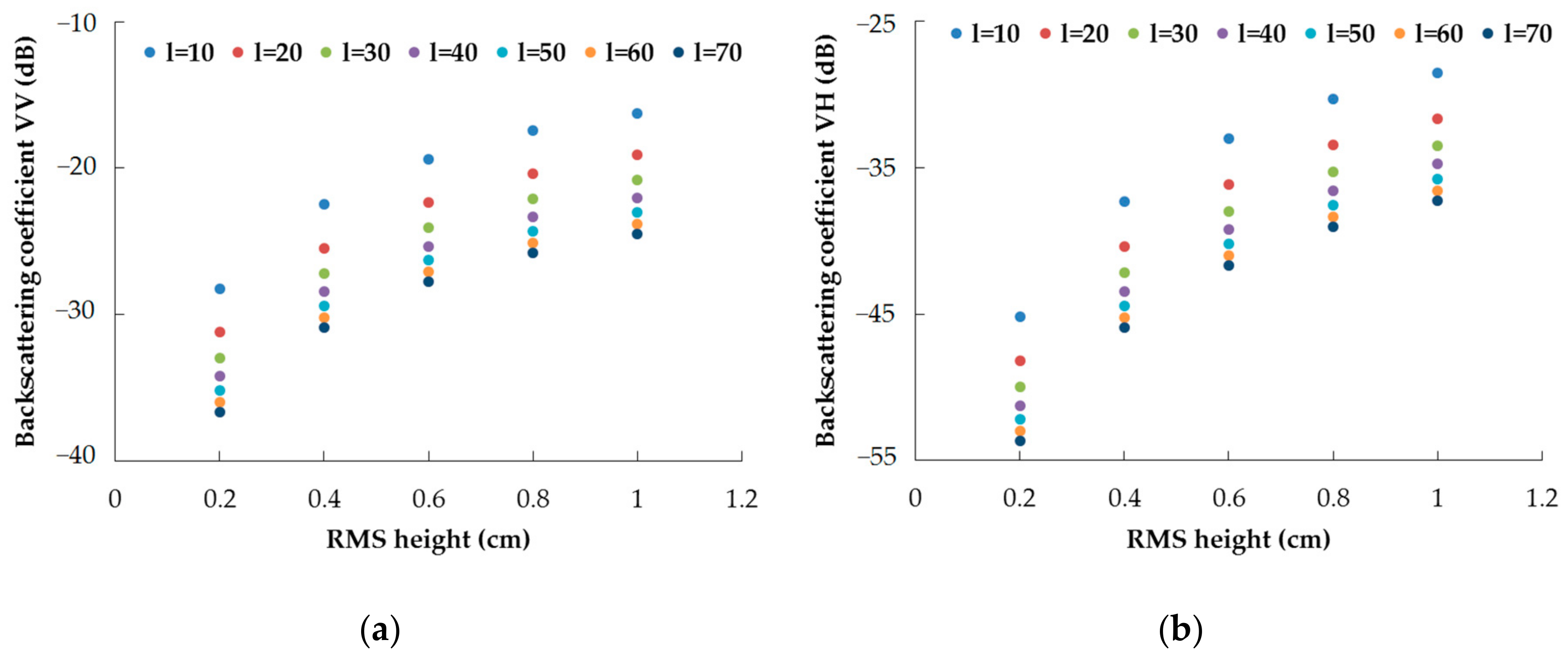
Relationship between Backscattering Coefficients and Surface Roughness

In order to simulate the functional relationship between backscattering coefficients and surface roughness, the parameter input ranges were limited by statistical analysis of the measured surface parameters in the study site: $\theta =45.08°$, ${\mathrm{m}}_{\mathrm{v}}=20\%$, $s\in \left[0.2,1.0\right]$ cm, and the step length of $s$ was 0.2 cm, $l\in \left[10,70\right]$ cm, and the step length of $l$ was 5 cm. The AIEM and the cross-polarized ratio of the Oh model were used to simulate the VV/VH backscattering coefficients under different roughness conditions to obtain a simulated data set.

Figure 2 shows the responses between the VV/VH polarization backscattering coefficients and RMS height under different correlation lengths (10, 20, 30, 40, 50, 60, and 70 cm). It can be seen that it is difficult to describe the response relationship between backscattering coefficients and roughness parameters by relying on a single roughness parameter (RMS height or correlation length). Multiple roughness parameters need to be considered simultaneously. The combined roughness parameters with different expressions have been widely used for soil moisture retrieval in recent years. In this paper, the combined roughness parameter $z_s$ proposed by Zribi et al. [28] ($z_s=s^2/l$) was selected to describe the surface roughness, taking into account the effects of RMS height and correlation length. When the radar system parameters are fixed, the larger the RMS height or the smaller the correlation length, the larger the combined roughness and the rougher the corresponding real surface, and vice versa.

Figure 3 illustrates the responses between the VV/VH polarization backscattering coefficients and the combined roughness $z_s$. It can be found that the backscattering coefficients increase with the increase of the combined roughness when the soil moisture is fixed, and there is an obvious logarithmic relationship within the range of simulation. When the combined roughness increases to a certain level, the backscattering coefficient gradually tends to stabilize.

Based on the above analysis, the general relationship between the backscattering coefficient and the combined roughness $z_s$ can be expressed as follows:

$${\sigma }_{qp}=a+b\ln \left(z_s\right)$$

(12)

where $a$ and $b$ are empirical parameters.

(2)

Relationship between Backscattering Coefficients and Soil Moisture

In order to simulate the functional relationship between the surface soil moisture and the backscattering coefficients, the parameter input ranges of AIEM were limited by statistical analysis of the measured surface parameters in the study site: $\theta =45.08°$, $s\in \left[0.2,1.0\right]$ cm, and the step length of $s$ was 0.2 cm, $l\in \left[10,70\right]$ cm, and the step length of $l$ was 5 cm, ${\mathrm{m}}_{\mathrm{v}}\in \left[5,60\right]$%, and the step length of ${\mathrm{m}}_{\mathrm{v}}$ was 5%. The AIEM and the cross-polarized ratio of the Oh model were used to simulate the variation of VV/VH backscattering coefficients with soil moisture under different roughness conditions to obtain a simulated dataset.

Figure 4 demonstrates the responses between the VV/VH polarization backscattering coefficients and soil moisture under different surface roughness. As shown in Figure 4, the backscattering coefficient has a similar variation law under different RMS height and correlation length. The backscattering coefficients increase with the increase of soil moisture when the roughness parameter is certain, and there is an obvious logarithmic relationship within the range of simulation. When the soil moisture increases to a certain level, the backscattering coefficient gradually tends to be stable.

The general relationship between the backscattering coefficient and soil moisture can be expressed as follows:

$${\sigma }_{qp}=c+d\ln \left(m_v\right)$$

(13)

where $c$ and $d$ are empirical parameters.

According to the above analysis, it is quite clear that when the radar incidence angle is constant, the comprehensive relationship between radar backscattering coefficient, surface roughness, and soil moisture can be obtained according to Equations (11)–(13):

$${\sigma }_{vv}=\left[a+b\ln \left(z_s\right)\right]\left[c+d\ln \left(m_v\right)\right]$$

(14)

Equation (14) can be written as follows:

$${\sigma }_{vv}=A\ln \left(z_s\right)+B\ln \left(m_v\right)+C\ln \left(z_s\right) \ln \left(m_v\right)+D$$

(15)

Likewise, a similar relationship can be obtained for VH polarization:

$${\sigma }_{vh}=E\ln \left(z_s\right)+F\ln \left(m_v\right)+G\ln \left(z_s\right) \ln \left(m_v\right)+H$$

(16)

The coefficients $A\sim H$ in Equations (15) and (16) are constants that can be determined by applying least square fitting method, so as to establish the empirical relationship between the dual-polarization backscattering coefficient, soil moisture and combined roughness. In this paper, the nonlinear equations composed of equations similar to Equations (15) and (16) are referred to be a new coupled empirical model (CEM), and the soil moisture can be collected by CEM.

According to the previous studies, although AIEM can effectively simulate the radar backscattering coefficient, there is still a certain deviation between the simulated radar backscattering and the actual radar backscattering, which is assumed to be caused by the measurement error of surface parameters. Based on the existing measurement methods, the measurement accuracy of soil moisture and RMS height can be guaranteed, while the measurement accuracy of correlation length is poor [31,32,33,34,35,36]. In this paper, the LUT (Look-up Tables) method proposed by Rahman et al. [52] was adopted to calculate the effective roughness parameters, which can avoid the introduction of uncertainty in the measurement process of roughness parameters. The simulated radar backscatter coefficient would be more consistent with the measured radar backscatter coefficient when the effective roughness is substituted for the measured roughness as input of CEM. Therefore, combined with the effective roughness as the input parameter, a new soil moisture inversion method based on the MWCM and CEM (MWCM-CEM) was proposed for the wheat growth cycle.

4. Results and Discussion

4.1. Backscattering Correction Results of Vegetation

On the basis of image segmentation, the radar backscattering coefficient and the vegetation information were extracted according to the geographical coordinates of sampling points. The influence of vegetation layer on radar backscattering was corrected by using WCM and MWCM, respectively. The changes of the backscattering coefficients of VH/VV polarization before and after the removal of the vegetation influence is fitted based on the data from April to June in the study site, as shown in Figure 5.

As revealed by Figure 5, the backscattering coefficients of different polarizations had different degrees of attenuation after WCM or MWCM treatment, which removed the effects of vegetation layer on the radar backscattering to a certain extent. Furthermore, the attenuation degree after being processed by MWCM was less than that of WCM. Due to the lack of truth value of bare soil backscattering coefficient, we cannot judge which one is better directly. In this regard, we will indirectly judge by the following soil moisture inversion results in Section 4.2. Despite the lack of a suitable optical data source in March 2013, it could be found that the vegetation fraction in this phase is low (NDVI < 0.3) based on the optical data in March of those years close to 2013. That is to say, the effects of the vegetation layer on radar backscattering coefficient is negligible. As a result, the radar backscattering coefficient in March is directly regarded as the bare soil backscattering coefficient.

From Figure 5, it can be found that the changes of backscattering coefficient before and after vegetation effect removal are small, owing to the low vegetation fraction in April. In May and June, especially in May, when the vegetation fraction is high, the backscattering coefficients change greatly. It is coincident with the theory of WCM and our a priori knowledge. In addition, the VH polarization data have a larger variation range than the VV polarization, indicating that the VH polarization signal is more sensitive to vegetation than VV.

4.2. Soil Moisture Inversion and Result Verification

To illustrate the improvement effect of MWCM compared with WCM and the necessity of replacing in-situ measurement roughness with effective roughness, four configurations of soil moisture inversion during the wheat growth cycle were discussed:

• Case 1: A combination of classical WCM and CEM obtained by least square fitting using field measured roughness and measured soil moisture (CEM_mr) (WCM-CEM_mr).
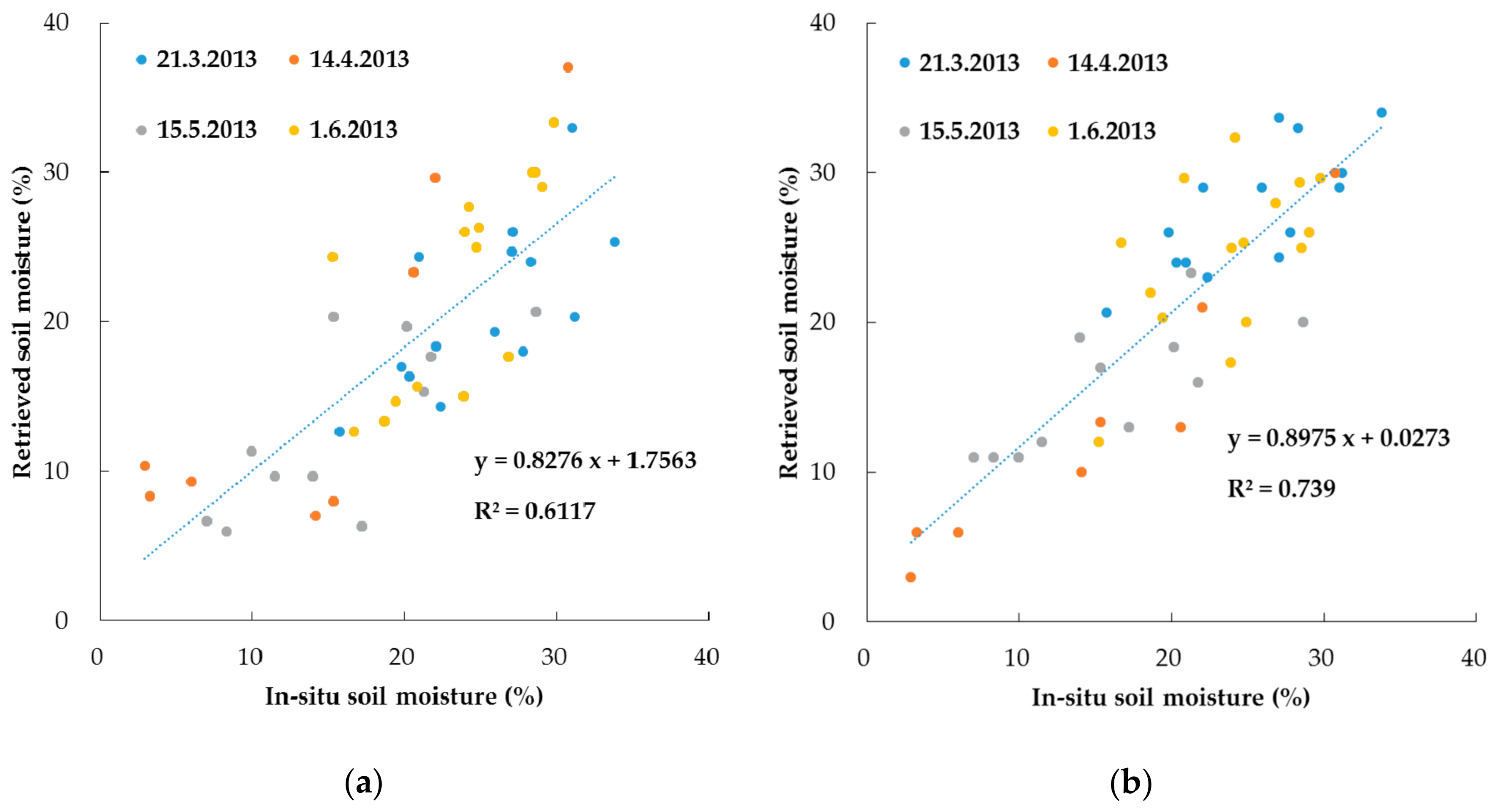
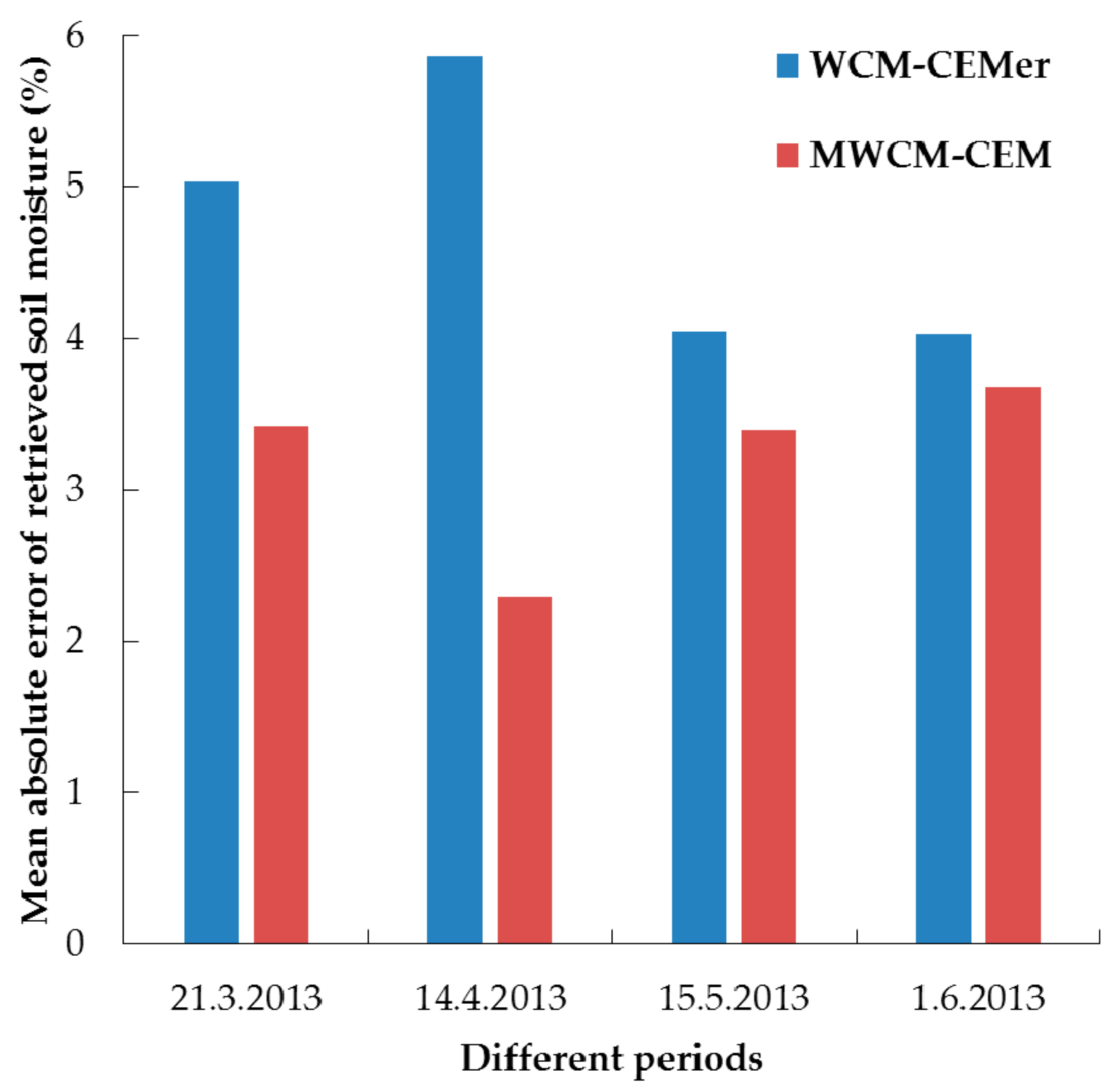
• Case 2: A combination of classical WCM and CEM obtained by least square fitting using effective roughness and measured soil moisture (CEM_er) (WCM-CEM_er).
• Case 3: A combination of MWCM and CEM_mr (MWCM-CEM_mr).
• Case 4: A combination of MWCM and CEM_er (MWCM-CEM, the method proposed in this paper).

In order to verify the feasibility of the above four combinations, the in-situ measurements data were used to compare and analyze the model forward and inversion results. Training data and validation data were randomly generated from 161 surface sampling points. Among them, 113 training samples were selected to establish the model and obtain the model coefficients (

Table 2. Coefficients fitted by least square method for four configurations.

	A	B	C	D	E	F	G	H
WCM-CEMmr	−2.007	−3.268	−0.965	−26.650	−4.441	−10.090	−2.448	−46.880
WCM-CEMer	3.912	4.622	0.349	−3.878	4.239	5.065	0.132	−10.690
MWCM-CEMmr	−1.294	−0.393	−0.340	−22.350	−3.362	−5.861	−1.530	−40.430
MWCM-CEM	4.083	5.247	0.0611	2.090	4.983	5.123	0.036	−8.005

), and the remaining 48 samples were used to verify the accuracy of the soil moisture retrieval model. Both the training samples and validation samples can provide soil moisture levels from low to high, where the high soil moisture may be due to precipitation or irrigation.

Figure 6 gives the fitting relationships between the backscattering coefficients simulated by AIEM and the ones calculated by the four combinations. As shown in Figure 6, when the field measured surface roughness were used as the input parameters of CEM, although the accuracy of MWCM-CEM_mr was slightly higher than that of WCM-CEM_mr, the forward modeling accuracies of WCM-CEM_mr and MWCM-CEM_mr were poor. The simulated backscattering coefficients were distributed in a narrow range, indicating that the randomness in the acquisition of surface roughness had a great influence on the simulation of radar backscattering coefficient. When the effective roughness was used as the input parameter of CEM, the forward accuracies of WCM-CEM_er and MWCM-CEM were better, and the accuracy of MWCM-CEM was slightly higher than that of WCM-CEM_er. The simulated backscattering coefficients were distributed in a wide range and highly agreed with the simulated values of AIEM. Therefore, it can be inferred that using effective roughness as the input of CEM instead of in-situ measured roughness can effectively avoid the uncertainty of roughness measurement on complex surface and greatly improve the simulation results. Due to the observation scale or other reasons, some errors occurred in the process of obtaining the surface roughness. The measured surface roughness parameters would introduce large errors to the simulated backscattering coefficient, which cannot be ignored in soil moisture inversion. Therefore, it was not considered to use case 1 and case 3 for the subsequent soil moisture inversion.

The coefficient of determination ($R^2$) between CEM_er simulation results and AIEM simulation values is above 0.94 (WCM-CEM_er: $R_{vh}^2=0.9784$,$R_{vv}^2=0.9434$; MWCM-CEM: $R_{vh}^2=0.9825$,$R_{vv}^2=0.9569$), which indicates that CEM_er can achieve high forward accuracy and preliminarily verifies the reliability of the model. Compared with the AIEM, the CEM_er mainly considers the influence of soil moisture and surface roughness on radar backscattering. Except for ensuring the simulation accuracy, the parameters of CEM_er are simple and easy to settle.

In order to further verify the validity of the soil moisture inversion method proposed in this paper, the 48 verification points were used to establish a comparative relationship between soil moisture retrieved values and measured values, as shown in Figure 7. The verification points were distributed uniformly in each phase, and the sampling points in different phases were indicated by different colors. From Figure 7, we can find that acceptable soil moisture inversion results can be obtained no matter using WCM-CEM_er or MWCM-CEM. The inversion results of MWCM-CEM were superior to WCM-CEM_er, with the $R^2$ reaching 0.7390, indicating that MWCM with vegetation fraction can improve the accuracy of soil moisture inversion effectively. According to the inversion results of MWCM-CEM, the absolute error of soil moisture in most of the 48 verification points is within 5%. MWCM-CEM did not show a large deviation for high soil moisture. Therefore, precipitation or irrigation have little impact on the accuracy of the inversion method in this paper, which proves that MWCM-CEM has a certain robustness. The root mean square error (RMSE) of the retrieved soil moisture and the measured value is 4.14%, which indicates that MWCM-CEM has good correlation and small errors. Figure 8 compared the mean absolute errors of soil moisture retrieved by WCM-CEMer and MWCM-CEM in each period. From Figure 8, it can be found that the inversion results of MWCM-CEM are better than that of WCM-CEMer in each period, especially in March and April when the study site is under low vegetation fraction. Therefore, compared with WCM, MWCM can describe the real surface vegetation coverage more accurately.

For the purpose of studying the changes of soil moisture in each important period of the wheat growth cycle, and further verifying the application effect of this method in non-sampling area through qualitative evaluation, MWCM-CEM was used for soil moisture inversion in the study site. The spatial distribution maps of soil moisture with different phases were obtained as shown in Figure 9. The blank parts of the maps are the abnormal value area of soil moisture inversion and artificial building plot area, such as urban construction land, highway, river, and so on. From Figure 9, it can be found that the soil moisture in the four periods of the study site mainly concentrated in $10–25\%$.

With the temperature rising in spring, the winter wheat in the study site entered the returning green stage in March, which belonged to the stage of low vegetation fraction ($f_{veg}<30\%$) [53]. In order to revive winter wheat and make it grow, irrigation is generally carried out during this period. According to Figure 9a, the soil moisture remains at a relatively high level, which is consistent with our a priori knowledge.

The winter wheat was in the jointing stage in April, belonging to the medium-low and medium vegetation fraction stage ($30\%\le f_{veg}<60\%$) [53], when the wheat grew vigorously, and the water consumption increased sharply. The second irrigation of winter wheat would be carried out at the end of April or the beginning of May to ensure the water demand of plants.

In May, the winter wheat in the study site had entered the filling stage, which belonged to the stage of high vegetation fraction ($75\%\le f_{veg}<1$) [53]. By comparing the inversion results of the red frame position of (a), (b), (c), and (d) in Figure 9, it can be revealed that there were some outliers in areas with high vegetation fraction, leading to fragmentation of the soil moisture map at the red frame position. MWCM-CEM had limitations in high vegetation fraction areas. It is likely that the C-band SAR is difficult to penetrate the dense vegetation, resulting in the radar backscatter information obtained in the high vegetation fraction areas only containing a small amount of ground information or not containing any, and could not be used for soil moisture retrieval. There also exists a possibility that MWCM can not completely remove the effects of vegetation in high vegetation fraction areas. It may be caused by the saturation of vegetation water content estimated by the spectral index method.

The winter wheat was in a milky maturity stage in June and belonged to the medium and medium-high vegetation fraction stage ($50\%\le f_{veg}<80\%$) [53]. The precipitation in the study site is mainly concentrated in June to September based on local meteorological data. Attributed to the rapid increase of precipitation in June and the vegetation growth will increase soil moisture retention, the soil moisture in the study site will remain at a high level. As can be seen from Figure 9, the soil moisture in the study site was the highest in June, which was consistent with the actual situation, further demonstrating the effectiveness of the MWCM-CEM.

According to the inversion results of soil moisture in different phases, it can be concluded that the MWCM-CEM is suitable for the whole wheat growth cycle. However, the inversion accuracy of soil moisture will decrease in the period of high vegetation fraction. There are two possible ways to solve the problem. The first way is to use L-band or other longer-band SAR data in the case of high vegetation fraction and use multi-band SAR data to monitor soil moisture changes during the crop growth cycle. The second one is to try other methods to calculate vegetation water content or to use other vegetation descriptors in MWCM. This problem will be further discussed in the follow-up work.

5. Conclusions

In this paper, MWCM, which introduced the vegetation fraction to WCM, was used for vegetation effects removal. The effective roughness parameter and the combined roughness form were used to describe the surface roughness. It avoids the uncertainty in the measurement of roughness parameters, and at the same time solves the problem that the measurement accuracy and efficiency are difficult to compromise caused by the anisotropy of surface roughness and spatial heterogeneity. Combined with MWCM, AIEM and the Oh model, a new soil moisture inversion method, MWCM-CEM, was established and realized soil moisture inversion during the wheat growth cycle in collaboration with Radarsat-2 active microwave data and Landsat-8 optical data in Dingxing County, Hebei Province.

The results indicated that, overall, the combination of MWCM and the CEM has a high soil moisture retrieval accuracy, with the $R^2$ = 0.7390 and the total RMSE = 4.14%. MWCM-CEM was used to obtain the soil moisture of the study site in March, April, May, and June, 2013, which basically covered the important stages of winter wheat growth and development. The characteristics of soil moisture temporal variation during crop growth was analyzed. It is helpful to provide references for irrigation and drought monitoring in agricultural production. In the further work, we will explore from the following aspects:

• In view of the complexity of actual soil types and land cover types, the applicability of MWCM-CEM needs to be further verified. The problem of soil moisture accuracy reduction in high vegetation fraction areas was discussed in this work. Multi-band SAR data will be comprehensively used to establish a soil moisture remote sensing inversion algorithm that meets regional characteristics, thereby improving the accuracy of soil moisture inversion.
• There are scale problems in using TDR point measurement data to verify remote sensing pixel inversion results. The cosmic ray neutron method can obtain the soil moisture in a certain region by measuring the intensity of the fast neutrons moderated by collision with hydrogen atoms. Its measuring range is between a TDR point measurement and a remote sensing method, which fills the gap in the measurement scale of soil moisture. Therefore, the cosmic ray neutron method can be used as an important and effective verification method for remote sensing inversion of soil moisture on the pixel scale in the subsequent studies.
• The microwave remote sensing method is only applicable to the acquisition of surface soil moisture, but cannot directly obtain the deep soil moisture information. On this basis, we will attempt to establish the relationship between surface soil moisture and deep soil moisture through physical models or mathematical methods in further research, so as to obtain soil moisture at different depths to meet the requirements.

References

1. Özerdem, M.; Acar, E.; Ekinci, R. Soil Moisture Estimation over Vegetated Agricultural Areas: Tigris Basin, Turkey from Radarsat-2 Data by Polarimetric Decomposition Models and a Generalized Regression Neural Network. Remote Sens. 2017, 9, 395. [Google Scholar] [CrossRef] [Green Version]
2. Kumar, S.; Dirmeyer, P.; Peters-Lidard, C.; Bindlish, R.; Bolten, J. Information Theoretic Evaluation of Satellite Soil Moisture Retrievals. Remote Sens. Environ. 2018, 204, 392–400. [Google Scholar] [CrossRef] [PubMed] [Green Version]
3. El Hajj, M.; Baghdadi, N.; Zribi, M. Comparative Analysis of the Accuracy of Surface Soil Moisture Estimation from the C- and L-Bands. Int. J. Appl. Earth Obs. Geoinf. 2019, 82, 101888. [Google Scholar] [CrossRef]
4. Yadav, V.; Prasad, R.; Bala, R.; Vishwakarma, A. An Improved Inversion Algorithm for Spatio-Temporal Retrieval of Soil Moisture through Modified Water Cloud Model Using C-Band Sentinel-1A SAR Data. Comput. Electron. Agric. 2020, 173, 105447. [Google Scholar] [CrossRef]
5. Zhang, X.; Chen, B.; Fan, H.; Huang, J.; Zhao, H. The Potential Use of Multi-Band SAR Data for Soil Moisture Retrieval over Bare Agricultural Areas: Hebei, China. Remote Sens. 2016, 8, 7. [Google Scholar] [CrossRef] [Green Version]
6. Liu, Z.; Li, P.; Yang, J. Soil Moisture Retrieval and Spatiotemporal Pattern Analysis Using Sentinel-1 Data of Dahra, Senegal. Remote Sens. 2017, 9, 1197. [Google Scholar] [CrossRef] [Green Version]
7. Hachani, A.; Ouessar, M.; Paloscia, S.; Santi, E.; Pettinato, S. Soil Moisture Retrieval from Sentinel-1 Acquisitions in an Arid Environment in Tunisia: Application of Artificial Neural Networks Techniques. Int. J. Remote Sens. 2019, 40, 9159–9180. [Google Scholar] [CrossRef]
8. Ezzahar, J.; Ouaadi, N.; Zribi, M.; Elfarkh, J.; Aouade, G.; Khabba, S.; Er-Raki, S.; Chehbouni, A.; Jarlan, L. Evaluation of Backscattering Models and Support Vector Machine for the Retrieval of Bare Soil Moisture from Sentinel-1 Data. Remote Sens. 2020, 12, 72. [Google Scholar] [CrossRef] [Green Version]
9. Jagdhuber, T.; Hajnsek, I.; Bronstert, A.; Papathanassiou, K. Soil Moisture Estimation under Low Vegetation Cover Using a Multi-Angular Polarimetric Decomposition. IEEE Trans. Geosci. Remote Sens. 2013, 51, 2201–2215. [Google Scholar] [CrossRef]
10. Bourgeau-Chavez, L.; Leblon, B.; Charbonneau, F.; Buckley, J. Evaluation of Polarimetric Radarsat-2 SAR Data for Development of Soil Moisture Retrieval Algorithms over a Chronosequence of Black Spruce Boreal Forests. Remote Sens. Environ. 2013, 132, 71–85. [Google Scholar] [CrossRef]
11. Ulaby, F.; Batlivala, P. Optimum Radar Parameters for Mapping Soil Moisture. IEEE Trans. Geosci. Electron. 1976, GE-14, 81–93. [Google Scholar] [CrossRef]
12. Wu, T.; Chen, K. A Reappraisal of the Validity of the IEM Model for Backscattering from Rough Surfaces. IEEE Trans. Geosci. Remote Sens. 2004, 42, 743–753. [Google Scholar]
13. Fung, A.; Chen, K. An Update on the IEM Surface Backscattering Model. IEEE Geosci. Remote Sens. Lett. 2004, 1, 75–77. [Google Scholar] [CrossRef]
14. Chen, K.; Chen, K.; Li, Z.; Liu, Y. Extension and Validation of an Advanced Integral Equation Model for Bistatic Scattering from Rough Surfaces. Prog. Electromagn. Res. 2015, 152, 59–76. [Google Scholar] [CrossRef] [Green Version]
15. Zeng, J.; Chen, K.; Bi, H.; Zhao, T.; Yang, X. A Comprehensive Analysis of Rough Soil Surface Scattering and Emission Predicted by AIEM with Comparison to Numerical Simulations and Experimental Measurements. IEEE Trans. Geosci. Remote Sens. 2017, 55, 1696–1708. [Google Scholar] [CrossRef]
16. Oh, Y.; Sarabandi, K.; Ulaby, F. An Empirical Model and an Inversion Technique for Radar Scattering from Bare Soil Surfaces. IEEE Trans. Geosci. Remote Sens. 1992, 30, 370–381. [Google Scholar] [CrossRef]
17. Oh, Y.; Sarabandi, K.; Ulaby, F. Semi-Empirical Model of the Ensemble-Averaged Differential Mueller Matrix for Microwave Backscattering from Bare Soil Surfaces. IEEE Trans. Geosci. Remote Sens. 2002, 40, 1348–1355. [Google Scholar] [CrossRef] [Green Version]
18. Oh, Y. Quantitative Retrieval of Soil Moisture Content and Surface Roughness from Multi-polarized Radar Observations of Bare Soil Surfaces. IEEE Trans. Geosci. Remote Sens. 2004, 42, 596–601. [Google Scholar] [CrossRef]
19. Dubois, P.; Van Zyl, J.; Engman, T. Measuring Soil Moisture with Imaging Radars. IEEE Trans. Geosci. Remote Sens. 1995, 33, 915–926. [Google Scholar] [CrossRef] [Green Version]
20. Chen, K.; Yen, S.; Huang, W. A Simple Model for Retrieving Bare Soil Moisture from Radar-scattering Coefficients. Remote Sens. Environ. 1995, 54, 121–126. [Google Scholar] [CrossRef]
21. Shi, J.; Wang, J.; Hsu, A.; O’Neill, P.; Engman, E. Estimation of Bare Surface Soil Moisture and Surface Roughness Parameter Using L-band SAR Image Data. IEEE Trans. Geosci. Remote Sens. 1997, 35, 1254–1266. [Google Scholar]
22. Pasolli, L.; Notarnicola, C.; Bertoldi, G.; Della Chiesa, S.; Niedrist, G.; Bruzzone, L.; Tappeiner, U.; Zebisch, M. Soil Moisture Monitoring in Mountain Areas by Using High-Resolution SAR Images: Results from a Feasibility Study. Eur. J. Soil Sci. 2014, 65, 852–864. [Google Scholar] [CrossRef]
23. Paloscia, S.; Pettinato, S.; Santi, E.; Notarnicola, C.; Pasolli, L.; Reppucci, A. Soil Moisture Mapping Using Sentinel-1 Images: Algorithm and Preliminary Validation. Remote Sens. Environ. 2013, 134, 234–248. [Google Scholar] [CrossRef]
24. Ahmad, S.; Kalra, A.; Stephen, H. Estimating Soil Moisture Using Remote Sensing Data: A Machine Learning Approach. Adv. Water Resour. 2010, 33, 69–80. [Google Scholar] [CrossRef]
25. Han, L.; Wang, C.; Yu, T.; Gu, X.; Liu, Q. High-Precision Soil Moisture Mapping Based on Multi-Model Coupling and Background Knowledge, Over Vegetated Areas Using Chinese GF-3 and GF-1 Satellite Data. Remote Sens. 2020, 12, 2123. [Google Scholar] [CrossRef]
26. Kornelsen, K.; Coulibaly, P. Advances in Soil Moisture Retrieval from Synthetic Aperture Radar and Hydrological Applications. J. Hydrol. 2013, 476, 460–489. [Google Scholar] [CrossRef]
27. Kong, J.; Yang, J.; Zhen, P.; Li, J.; Yang, L. A Coupling Model for Soil Moisture Retrieval in Sparse Vegetation Covered Areas Based on Microwave and Optical Remote Sensing Data. IEEE Trans. Geosci. Remote Sens. 2018, 56, 7162–7173. [Google Scholar] [CrossRef]
28. Zribi, M.; Dechambre, M. A New Empirical Model to Retrieve Soil Moisture and Roughness from C-band Radar Data. Remote Sens. Environ. 2003, 84, 42–52. [Google Scholar] [CrossRef]
29. Guo, S.; Bai, X.; Chen, Y.; Zhang, S.; Hou, H.; Zhu, Q.; Du, P. An Improved Approach for Soil Moisture Estimation in Gully Fields of the Loess Plateau Using Sentinel-1A Radar Images. Remote Sens. 2019, 11, 349. [Google Scholar] [CrossRef] [Green Version]
30. Huang, S.; Ding, J.; Zou, J.; Liu, B.; Zhang, J.; Chen, W. Soil Moisture Retrieval Based on Sentinel-1 Imagery under Sparse Vegetation Coverage. Sensors 2019, 19, 589. [Google Scholar] [CrossRef] [Green Version]
31. Su, Z.; Troch, P.; De Troch, F. Remote Sensing of Soil Moisture Using EMAC/ESAR Data. Int. J. Remote Sens. 1997, 18, 2105–2124. [Google Scholar] [CrossRef]
32. Bai, X.; He, B.; Li, X. Optimum Surface Roughness to Parameterize Advanced Integral Equation Model for Soil Moisture Retrieval in Prairie Area Using Radarsat-2 Data. IEEE Trans. Geosci. Remote Sens. 2016, 54, 2437–2449. [Google Scholar] [CrossRef]
33. Bai, X.; He, B.; Li, X.; Zeng, J.; Wang, X.; Wang, Z.; Zeng, Y.; Su, Z. First Assessment of Sentinel-1A Data for Surface Soil Moisture Estimations Using a Coupled Water Cloud Model and Advanced Integral Equation Model over the Tibetan Plateau. Remote Sens. 2017, 9, 714. [Google Scholar] [CrossRef] [Green Version]
34. Han, Y.; Bai, X.; Shao, W.; Wang, J. Retrieval of Soil Moisture by Integrating Sentinel-1A and MODIS Data over Agricultural Fields. Water 2020, 12, 1726. [Google Scholar] [CrossRef]
35. Lievens, H.; Verhoest, N. On the Retrieval of Soil Moisture in Wheat Fields from L-Band SAR Based on Water Cloud Modeling, the IEM, and Effective Roughness Parameters. IEEE Geosci. Remote Sens. Lett. 2011, 8, 740–744. [Google Scholar] [CrossRef]
36. Lievens, H.; Verhoest, N.; De Keyser, E.; Vernieuwe, H.; Matgen, P.; Alvarez-Mozos, J.; Baets, B. Effective Roughness Modelling as a Tool for Soil Moisture Retrieval from C-And L-Band SAR. Hydrol. Earth Syst. Sci. 2011, 15, 151–162. [Google Scholar] [CrossRef] [Green Version]
37. Attema, E.; Ulaby, F. Vegetation Modeled as a Water Cloud. Radio Sci. 1978, 13, 357–364. [Google Scholar] [CrossRef]
38. Ulaby, F.; Sarabandi, K.; McDonald, K.; Whitt, M.; Dobson, M. Michigan Microwave Canopy Scattering Model. Int. J. Remote Sens. 1990, 11, 1223–1253. [Google Scholar] [CrossRef]
39. Qiu, J.; Crow, W.; Wagner, W.; Zhao, T. Effect of Vegetation Index Choice on Soil Moisture Retrievals via the Synergistic Use of Synthetic Aperture Radar and Optical Remote Sensing. Int. J. Appl. Earth Obs. Geoinf. 2019, 80, 47–57. [Google Scholar] [CrossRef]
40. Li, J.; Wang, S. Using SAR-Derived Vegetation Descriptors in a Water Cloud Model to Improve Soil Moisture Retrieval. Remote Sens. 2018, 10, 1370. [Google Scholar] [CrossRef] [Green Version]
41. Baghdadi, N.; El Hajj, M.; Zribi, M.; Bousbih, S. Calibration of the Water Cloud Model at C-Band for Winter Crop Fields and Grasslands. Remote Sens. 2017, 9, 969. [Google Scholar] [CrossRef] [Green Version]
42. El Hajj, M.; Baghdadi, N.; Zribi, M.; Belaud, G.; Cheviron, B.; Courault, D.; Charron, F. Soil Moisture Retrieval over Irrigated Grassland Using X-Band SAR Data. Remote Sens. Environ. 2016, 176, 202–218. [Google Scholar] [CrossRef] [Green Version]
43. Yang, Z.; Li, K.; Shao, Y.; Brisco, B.; Liu, L. Estimation of Paddy Rice Variables with a Modified Water Cloud Model and Improved Polarimetric Decomposition Using Multi-Temporal RADARSAT-2 Images. Remote Sens. 2016, 8, 878. [Google Scholar] [CrossRef] [Green Version]
44. He, B.; Xing, M.; Bai, X. A Synergistic Methodology for Soil Moisture Estimation in an Alpine Prairie Using Radar and Optical Satellite Data. Remote Sens. 2014, 6, 10966–10985. [Google Scholar] [CrossRef] [Green Version]
45. Bindlish, R.; Barros, A. Parameterization of Vegetation Backscatter in Radar-Based, Soil Moisture Estimation. Remote Sens. Environ. 2001, 76, 130–137. [Google Scholar] [CrossRef]
46. Wang, Q.; Li, J.; Jin, T.; Chang, X.; Zhu, Y.; Li, Y.; Sun, J.; Li, D. Comparative Analysis of Landsat-8, Sentinel-2, and GF-1 Data for Retrieving Soil Moisture over Wheat Farmlands. Remote Sens. 2020, 12, 2708. [Google Scholar] [CrossRef]
47. Bao, Y.; Lin, L.; Wu, S.; Deng, K.; Petropoulos, G. Surface Soil Moisture Retrievals over Partially Vegetated Areas from the Synergy of Sentinel-1 and Landsat 8 Data Using a Modified Water-Cloud Model. Int. J. Appl. Earth Obs. Geoinf. 2018, 72, 76–85. [Google Scholar] [CrossRef]
48. Jackson, T.; Chen, D.; Cosh, M.; Li, F.; Anderson, M.; Walthall, C.; Doriaswamy, P.; Hunt, E. Vegetation Water Content Mapping Using Landsat Data Derived Normalized Difference Water Index for Corn and Soybeans. Remote Sens. Environ. 2004, 92, 475–482. [Google Scholar] [CrossRef]
49. Gao, Y.; Walker, J.; Allahmoradi, M.; Monerris, A.; Ryu, D.; Jackson, T. Optical Sensing of Vegetation Water Content: A Synthesis Study. IEEE J. Sel. Top. App. Earth Obs. Remote Sens. 2015, 8, 1456–1464. [Google Scholar]
50. Jiapaer, G.; Chen, X.; Bao, A. A Comparison of Methods for Estimating Fractional Vegetation Cover in Arid Regions. Agric. For. Meteorol. 2011, 151, 1698–1710. [Google Scholar] [CrossRef]
51. Choker, M.; Baghdadi, N.; Zribi, M.; El Hajj, M.; Paloscia, S.; Verhoest, N.; Lievens, H.; Mattia, F. Evaluation of the Oh, Dubois and IEM Backscatter Models Using a Large Dataset of SAR Data and Experimental Soil Measurements. Water 2017, 9, 38. [Google Scholar] [CrossRef]
52. Rahman, M.; Moran, M.; Thoma, D.; Bryant, R.; Sano, E.; Collins, C.; Skirbvin, S.; Kershner, C.; Orr, B. A Derivation of Roughness Correlation Length for Parameterizing Radar Backscatter Models. Int. J. Remote Sens. 2007, 28, 3995–4012. [Google Scholar] [CrossRef]
53. Zhao, L.; Zhang, R.; Liu, Y.; Zhu, Z. The Differences between Extracting Vegetation Information from GF1-WFV and Landsat8-OLI. Acta Ecol. Sin. 2020, 40, 3495–3506. [Google Scholar]
Figure 1. Location of the study region and the distribution of the sampling plots in the study site. The background image is a polarization composite image of RADARSAT-2 (R: VH, G: HV, B: HH) in the study area.
Water 13 00135 g001
Figure 2. Responses of the backscattering coefficients and RMS height under different correlation lengths (10, 20, 30, 40, 50, 60, and 70 cm) when the soil moisture is 20%: (a) VV polarization; (b) VH polarization.
Water 13 00135 g002
Figure 3. Responses of the backscattering coefficients and z s when the soil moisture is 20%: (a) VV polarization; (b) VH polarization.
Water 13 00135 g003
Figure 4. Responses of the backscattering coefficient and soil moisture under different roughness: (a,b) responses of the VV/VH under RMS heights s = 0.2, 0.4, 0.6, 0.8, and 1.0 cm when the correlation length l = 15 cm; (c,d) responses of the VV/VH under l = 10, 20, 30, 40, 50, 60, and 70 cm when s = 0.6 cm.
Water 13 00135 g004
Figure 5. The VV/VH polarization backscattering coefficients before and after the removal of vegetation influence in different phases: (a,b) 14.4.2013; (c,d) 15.5.2013; (e,f) 1.6.2013. The blue dots represent the original radar backscattering coefficients, while the red dots and green dots represent the radar backscattering coefficients after the removal of vegetation influence by WCM and MWCM, respectively.
Water 13 00135 g005
Figure 6. Comparison of simulated backscattering coefficients between AIEM and the four combinations: (a) WCM-CEMmr; (b) WCM-CEMer; (c) MWCM-CEMmr; (d) MWCM-CEM.
Water 13 00135 g006
Figure 7. Comparison of soil moisture between measured and retrieved under two combinations: (a) WCM-CEMer; (b) MWCM-CEM.
Water 13 00135 g007
Figure 8. Mean absolute error of soil moisture retrieved by WCM-CEMer and MWCM-CEM in each period.
Water 13 00135 g008
Figure 9. Spatial distribution maps of soil moisture in each period of the study site: (a) 21.3.2013; (b) 14.4.2013; (c) 15.5.2013; (d) 1.6.2013.
Water 13 00135 g009