
Behaviors of the Yukon River Sediment Plume in the Bering Sea: Relations to Glacier-Melt Discharge and Sediment Load

 ,
, 
Abstract
:1. Introduction
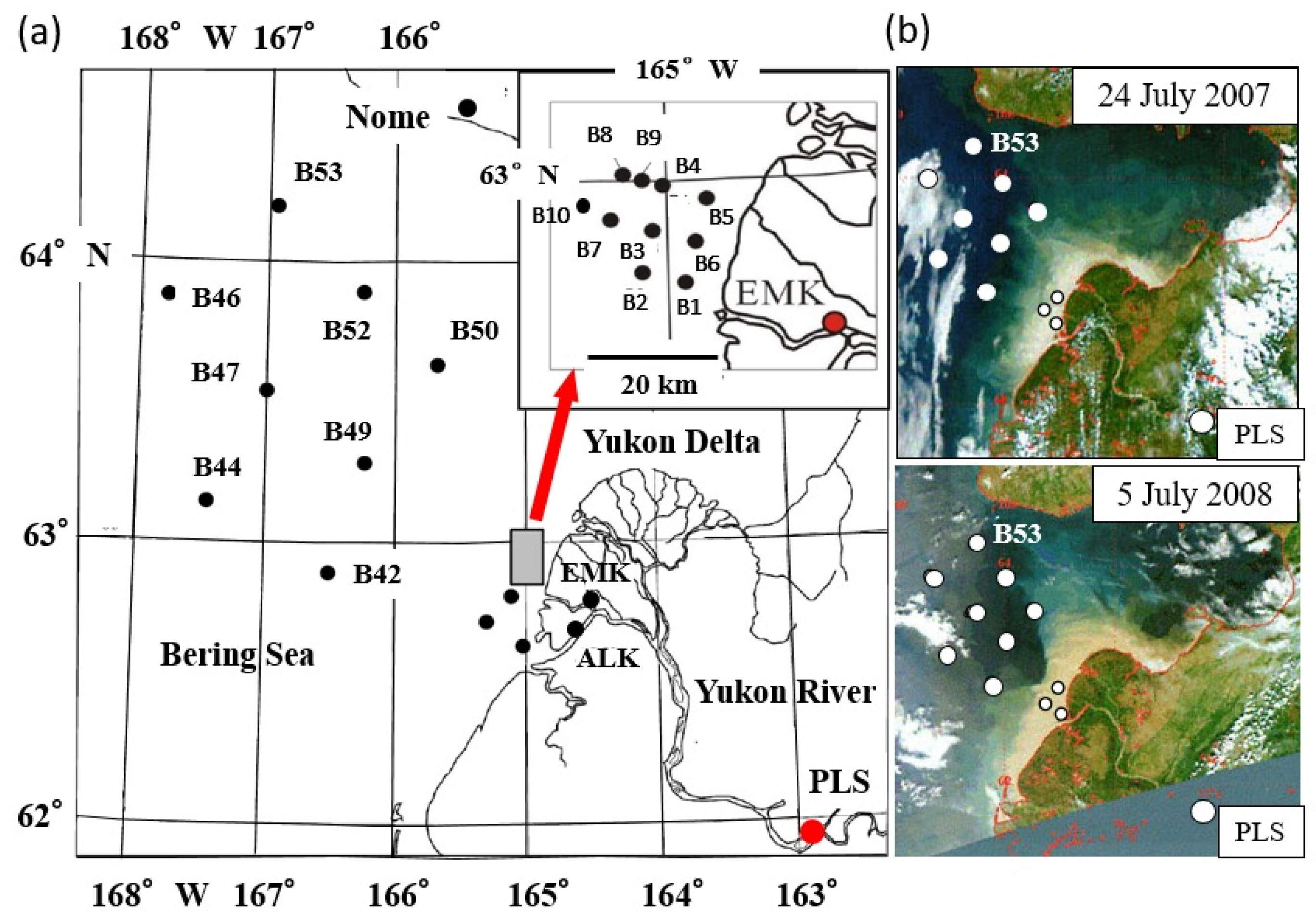
2. Study Area
3. Methods
3.1. Field Observations
3.2. Laboratory Experiments
3.3. Image Analysis
4. Results
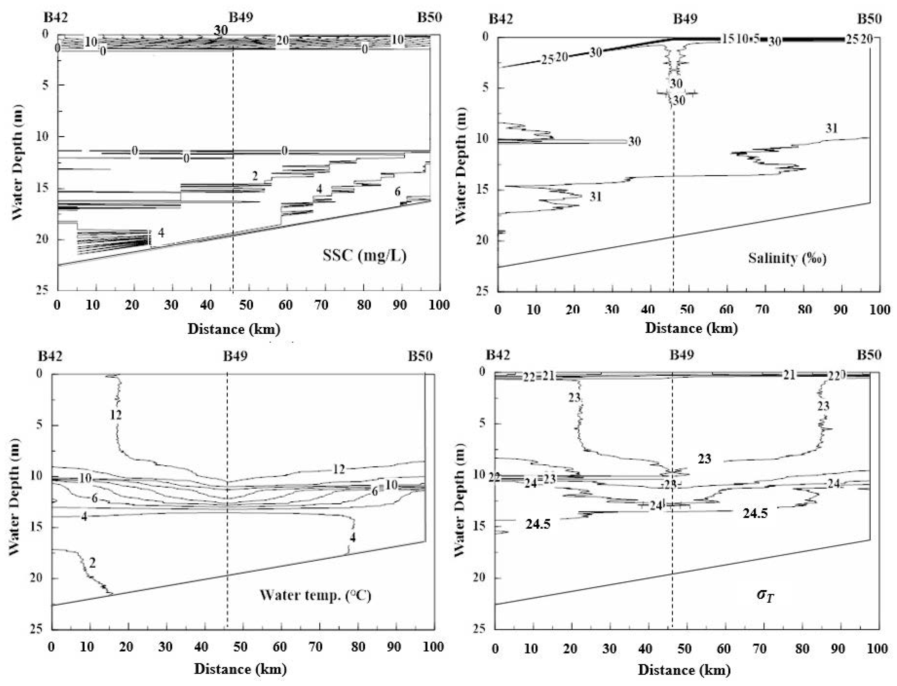
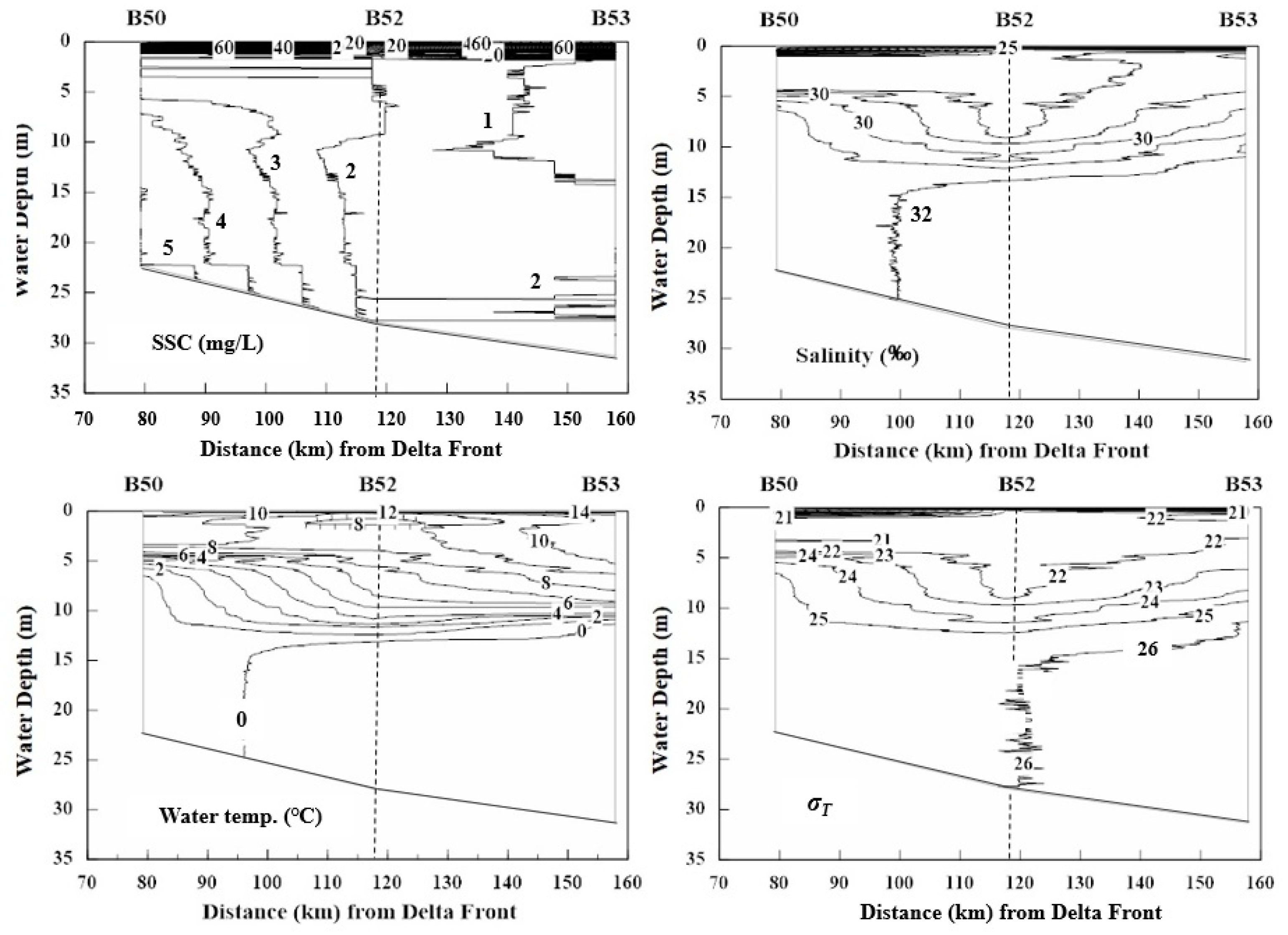
4.1. Sediment Plume Behaviors by Field Observations
4.2. Analytical Results for Grain Size of Bottom Sediment
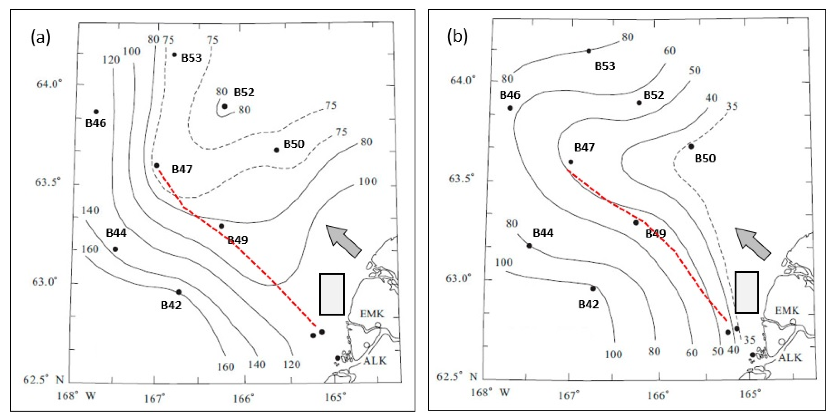
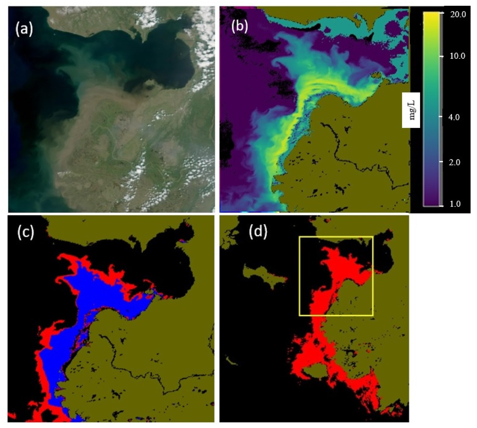
4.3. Analytical Results for the Satellite Images
5. Discussion
5.1. Dynamic Conditions of Yukon Sediment Plume from Field Observations
5.2. Behaviors of the Yukon River Sediment Plume Controlled by River Sediment Load
6. Conclusions
- (1)
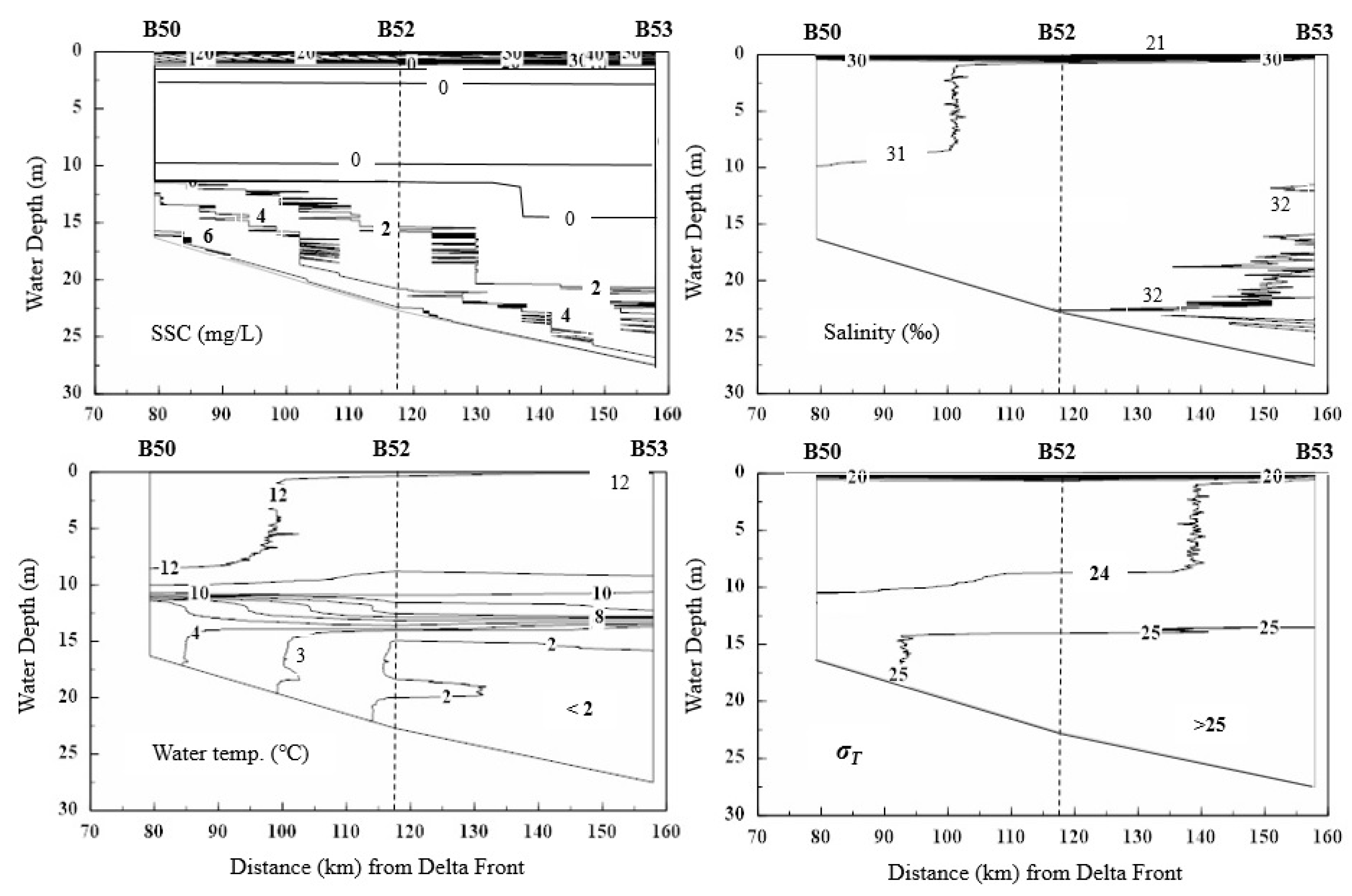
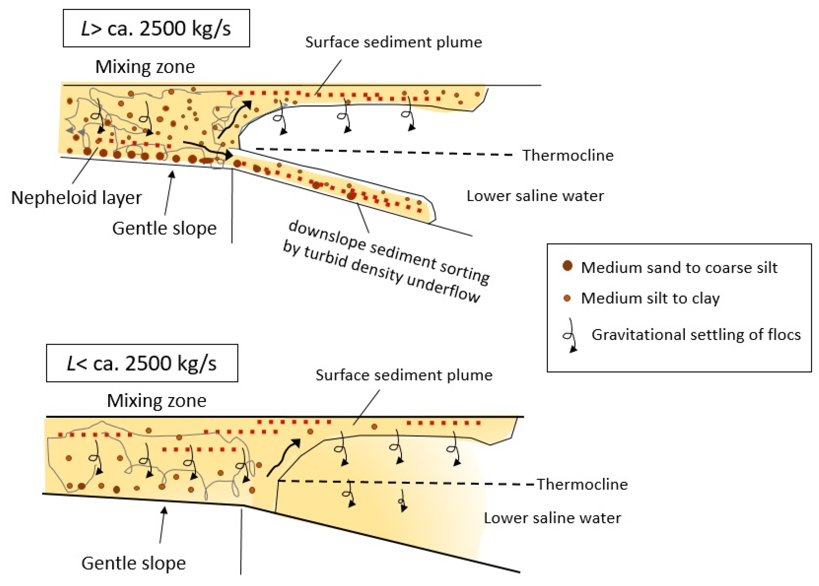
- The shipboard observation in 2007 suggested that, at the river sediment load of ca. 3000 kg/s, the turbid water in the coastal mixing zone is separated into the surface sediment plume and density underflow. Meanwhile, by the coastal observation in 2008, it was found out that, at the sediment load of ca. 2500 kg/s, the coastal mixed water is separated into the surface sediment plume and turbid density underflow. The separation into the surface plume and underflow could thus occur at the sediment load of more than ca. 2500 kg/s.
- (2)
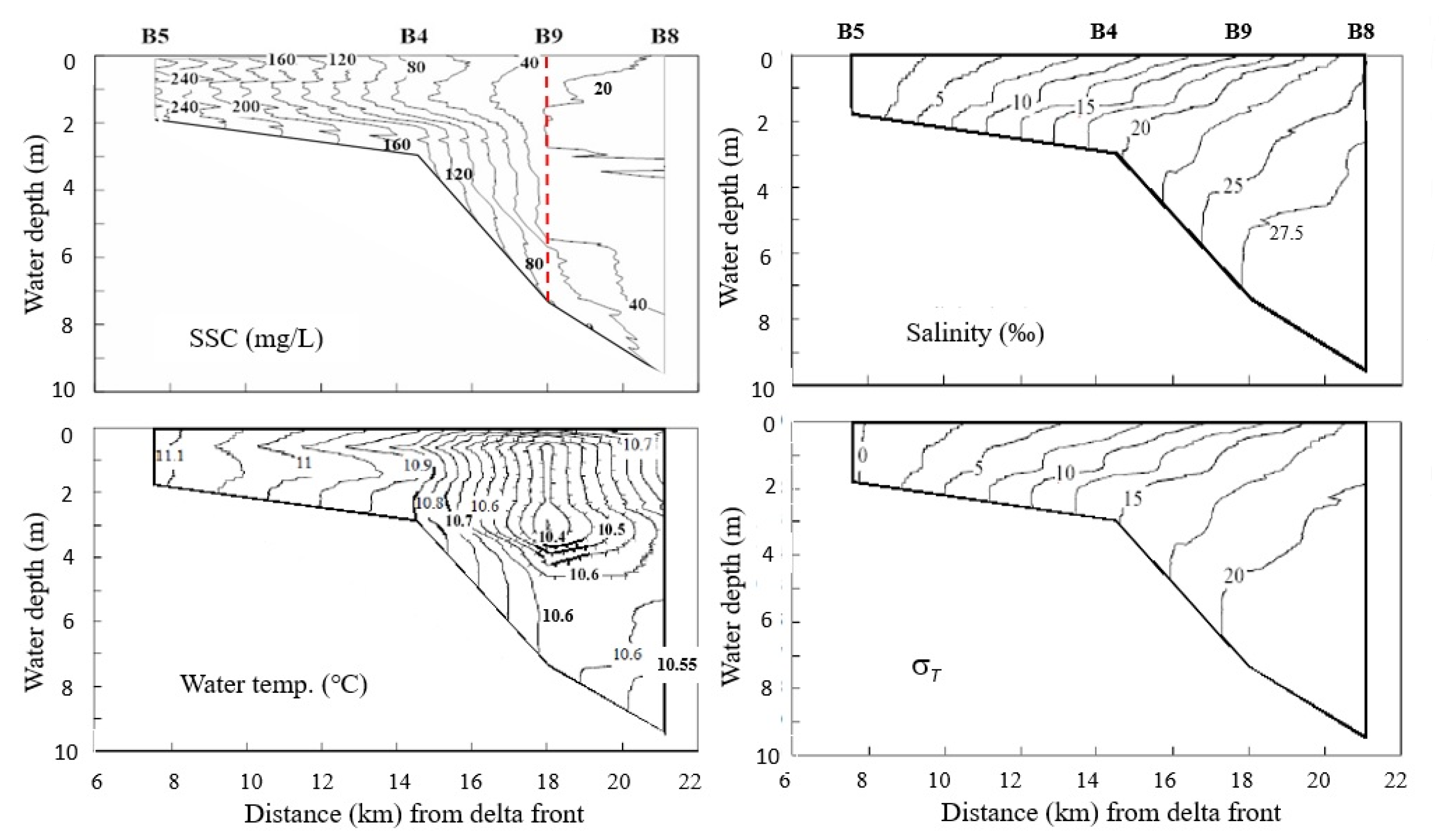
- In the shipboard observation in 2008, when the Yukon sediment load was 1600 kg/s on average, such a separation in (1) was not seen, and instead, sedimentation from the surface sediment plume prevailed in the lower whole layer. In the coastal observation in 2010, where the sediment load was ca. 2200 kg/s, neither a nepheloid layer nor density underflow was seen, and instead, the vertical mixing of turbid water prevailed extensively, showing the vertical uniform SSC and water temperature. Thus, the sediment load value at 2500 kg/s could be regarded as a criterion for changing the sedimentation in the coastal and offshore regions.
- (3)
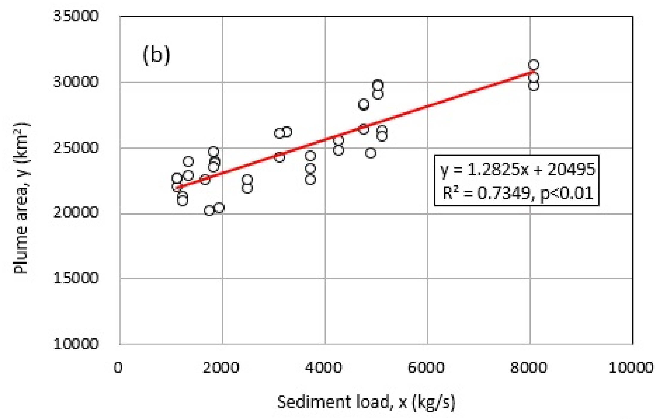
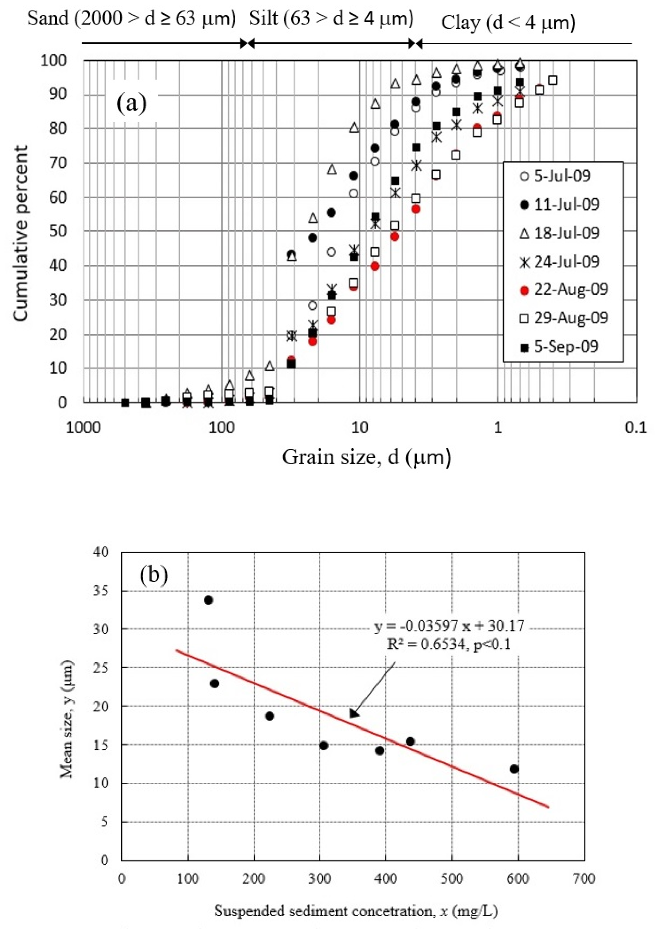
- Grain size distributions of bottom sediment in the coastal to offshore regions suggest that the sediment sorting by the turbid underflow shown in the above (1) occurred.
- (4)
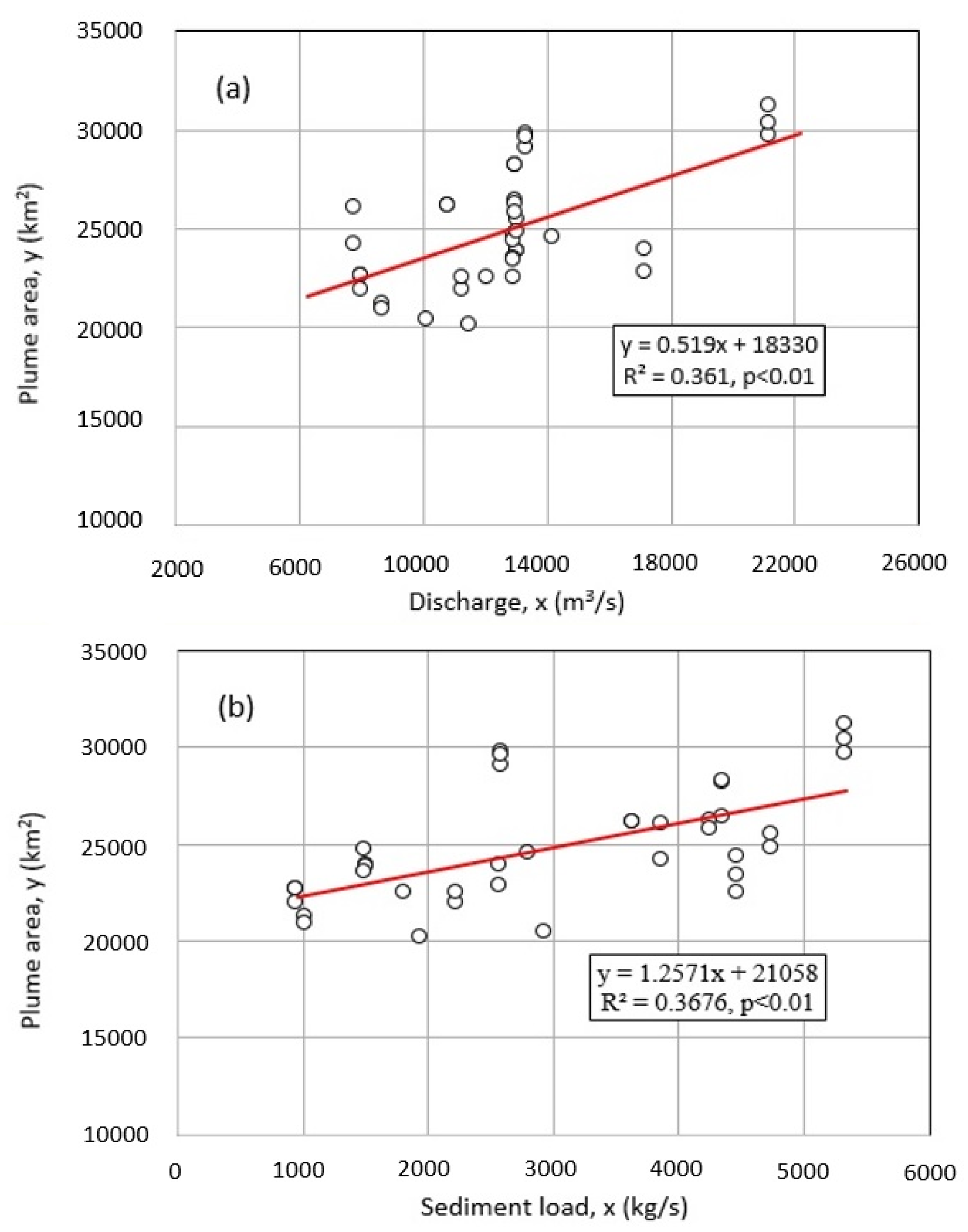
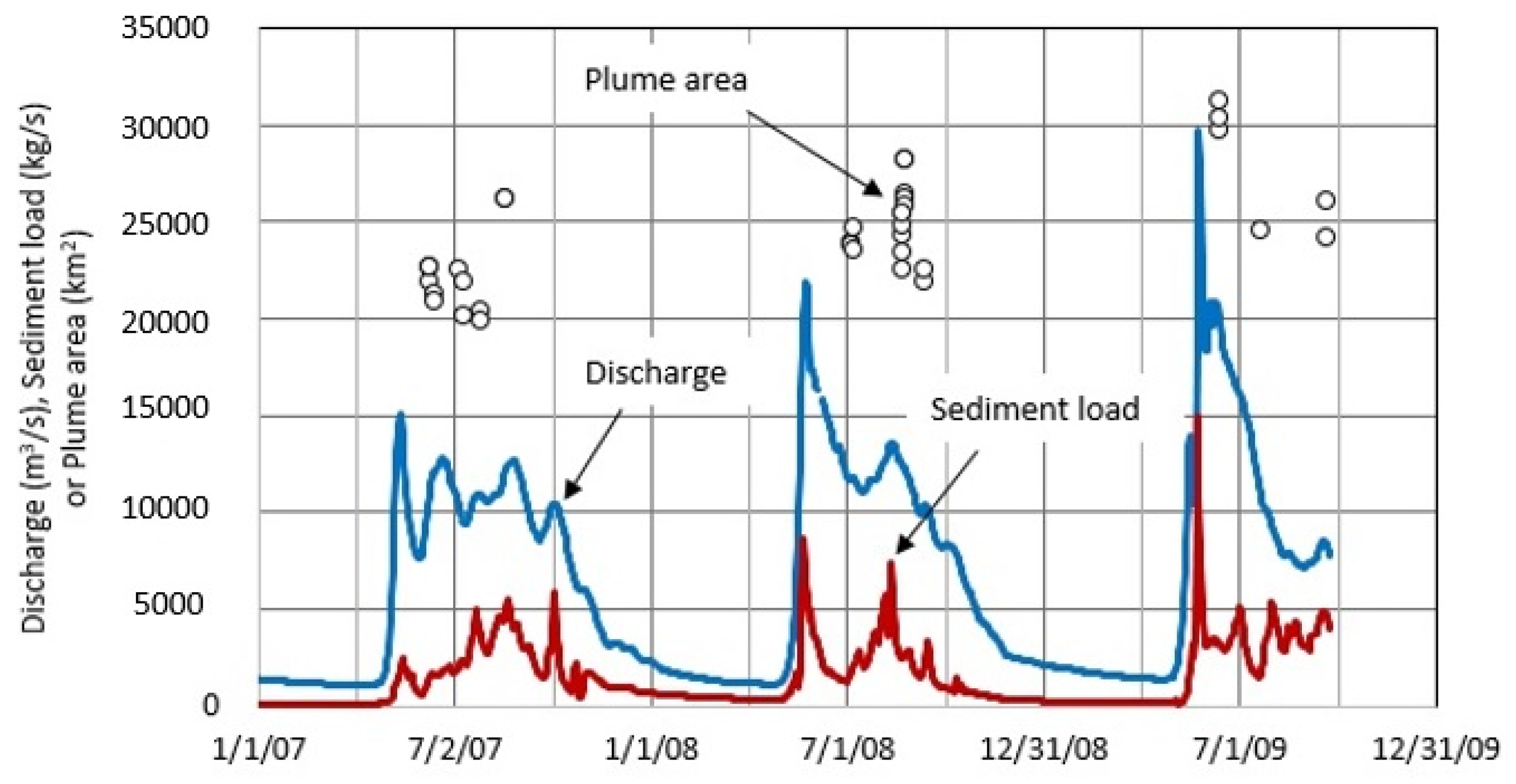
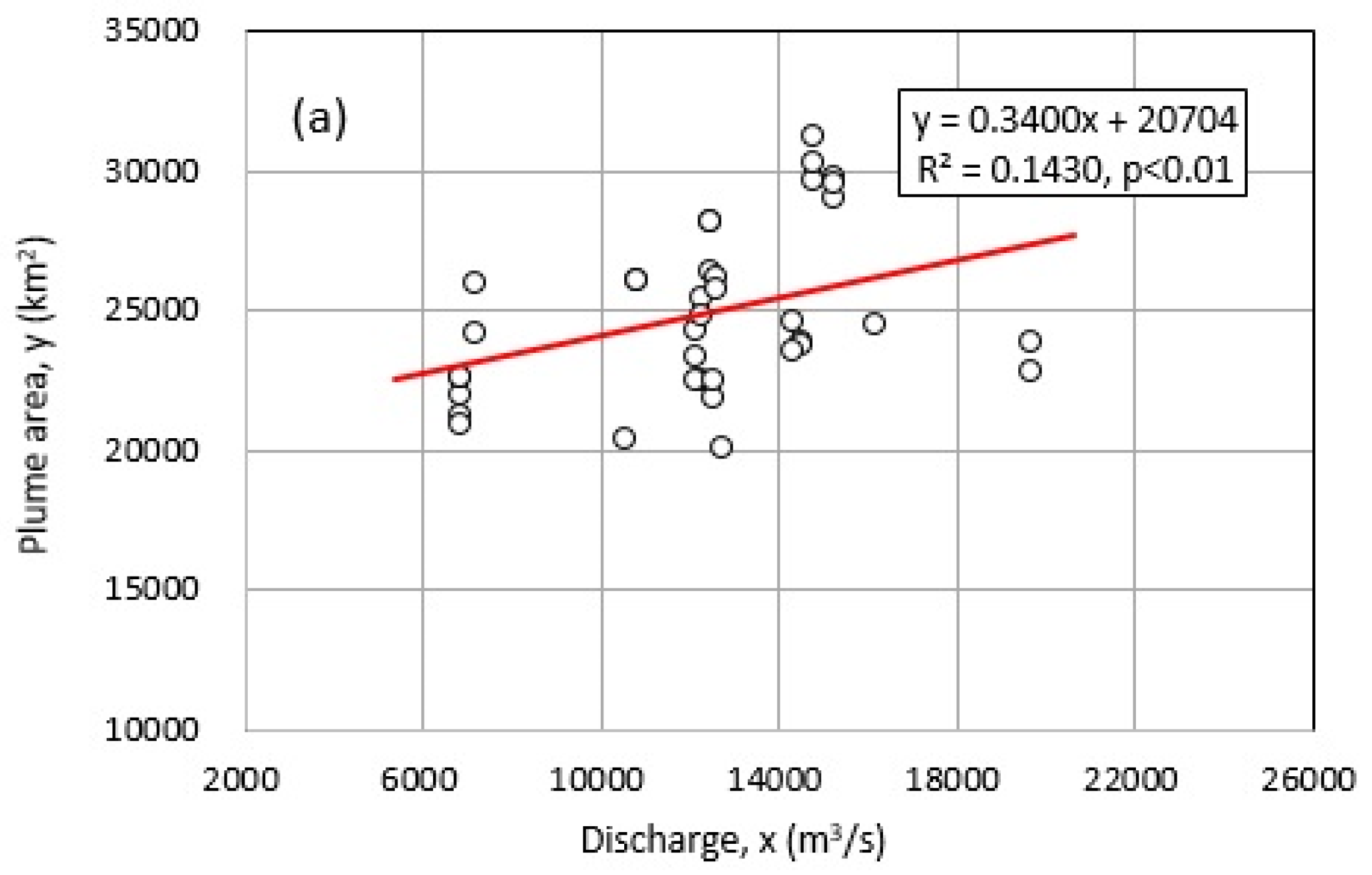
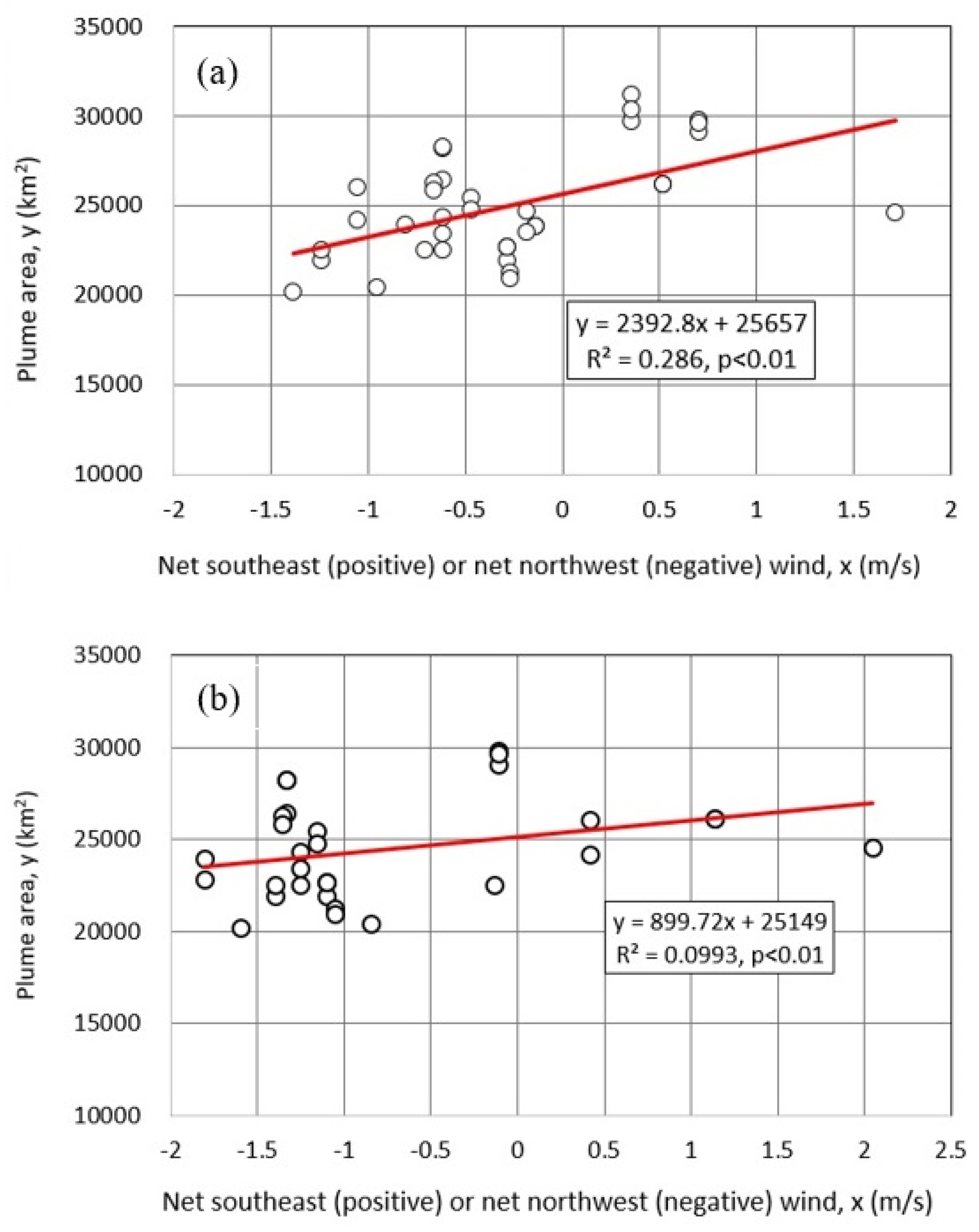
- There was a significant linear relationship (R2 = 0.735, p < 0.01) between the plume area and the sediment load averaged for two days delayed by 20 days and 21 days to the image dates. This suggests that the dispersion of surface sediment plumes in the Bering Sea is controlled by sediment runoff events of the Yukon River rather than “Alaskan Coastal Water”.
- (5)
- The dispersion of the surface plume is probably unaffected by the wind-driven currents because there is no significant correlation between the plume area and the net southeast wind or the net northwest wind in the corresponding periods.
Author Contributions
Funding
Institutional Review Board Statement
Informed Consent Statement
Data Availability Statement
Acknowledgments
Conflicts of Interest
References
- Branch, R.A.; Horner-Devine, A.R.; Kumar, N.; Poggioli, A.R. River plume liftoff dynamics and surface expressions. Water Res. Res. 2020, 56, e2019WR026475. [Google Scholar] [CrossRef]
- Guo, X.; Cai, W.-J.; Huang, W.-J.; Wang, Y.; Chen, F.; Murrell, M.C.; Lohrenz, S.E.; Jiang, L.-Q.; Dai, M.; Hartmann, J.; et al. Carbon dynamics and community production in the Mississippi River plume. Limnol. Oceanogr. 2012, 57, 1–17. [Google Scholar] [CrossRef]
- Chen, C.-C.; Gong, G.-C.; Chiang, K.-P.; Shiah, F.-K.; Chung, C.-C.; Hung, C.-C. Scaling effects of a eutrophic river plume on organic carbon consumption. Limnol. Oceanogr. 2021, 66, 1867–1881. [Google Scholar] [CrossRef]
- Mulder, T.; Syvitski, J.P.M.; Migeon, S.; Faugères, J.-C.; Savoye, B. Marine hyperpycnal flows: Initiation, behavior and related deposits: A review. Mar. Pet. Geol. 2003, 20, 861–882. [Google Scholar] [CrossRef]
- Horner-Devine, A.R.; Hetland, R.D.; MacDonald, D.G. Mixing and transport in coastal river plumes. Annu. Rev. Fluid Mech. 2015, 47, 569–594. [Google Scholar] [CrossRef]
- Chikita, K.; Yonemitsu, N.; Yoshida, M. Dynamic sedimentation processes in a glacier-fed lake, Peyto Lake, Alberta, Canada. Jpn. J. Limnol. 1991, 52, 27–43. [Google Scholar] [CrossRef] [Green Version]
- Chikita, K.; Sakata, K.; Hino, S. Transportation of suspended sediment slowly settling in a caldera lake. Jpn. J. Limnol. 1995, 56, 245–257. [Google Scholar] [CrossRef]
- Schiller, R.V.; Kourafalou, V.H.; Hogan, P.; Walker, N.D. The dynamics of the Mississippi River plume: Impact of topography, wind and offshore forcing on the fate of plume waters. J. Geophys. Res. 2011, 116, C06029. [Google Scholar] [CrossRef]
- Halverson, M.; Pawlowicz, R. Tide, wind, and river forcing of the surface currents in the Fraser River plume. Atmosphere-Ocean 2016, 54, 131–152. [Google Scholar] [CrossRef]
- Mulligan, R.P.; Perrie, W.; Solomon, S. Dynamics of the Mackenzie River plume on the inner Beaufort shelf during an open water period in summer. Estuar. Coast. Shelf Sci. 2010, 89, 214–220. [Google Scholar] [CrossRef]
- Gouveia, N.A.; Gherardi, D.F.M.; Aragão, L.E.O.C. The role of the Amazon River plume on the intensification of the hydrological cycle. Geophys. Res. Lett. 2019, 46, 12221–12229. [Google Scholar] [CrossRef]
- Masunaga, E.; Fringer, O.B.; Yamazaki, H. An observational and numerical study of river plume dynamics in Otsuchi Bay, Japan. Jour. Oceanogr. 2016, 72, 3–21. [Google Scholar] [CrossRef]
- Zavala, C. Hyperpycnal (over density) flows and deposits. J. Palaeogeogr. 2020, 9, 17. [Google Scholar] [CrossRef]
- Lick, W.; Huang, H.; Jepsen, R. Flocculation of fine-grained sediments due to differential settling. J. Geophys. Res. Ocean. 1993, 98, 10279–10288. [Google Scholar] [CrossRef]
- Strom, K.; Keybani, A. Flocculation in a decaying shear field and its implications for mud removal in near-field river mouth discharges. J. Geophys. Res. Oceans 2015, 121, 2142–2162. [Google Scholar] [CrossRef]
- Milligan, T.G.; Hill, P.S.; Law, B.A. Flocculation and the loss of sediment from the Po River plume. Cont. Shelf Res. 2007, 27, 309–321. [Google Scholar] [CrossRef]
- Marukussen, T.N.; Elberling, B.; Winter, C.; Andersen, T.J. Flocculated meltwater particles control Arctic land-sea fluxes of labile iron. Sci. Rep. 2016, 6, 24033. [Google Scholar] [CrossRef] [PubMed]
- Reimers, C.; Carl Friedrichs, C.; Bebout, B.; Howd, P.; Huettel, M.; Jahnke, R.; MacCready, P.; Ruttenberg, K.; Sanford, L.; Trowbridge, J. Coastal benthic exchange dynamics. In Skidaway Institute of Oceanography Technical Report TR-04-01; University of Georgia: Savannah, GA, USA, 2004; 92p. [Google Scholar]
- Wang, Z.; Li, W.; Zhang, K.; Agrawal, Y.C.; Huang, H. Observations of the distribution and flocculation of suspended particulate matter in the North Yellow Sea cold water mass. Cont. Shelf Res. 2020, 204, 104187. [Google Scholar] [CrossRef]
- Nelson, H.; Creager, J.S. Displacement of Yukon-derived sediment from Bering Sea to Chukchi Sea during Holocene time. Geology 1977, 5, 141–146. [Google Scholar] [CrossRef]
- Dean, K.G.; McRoy, C.P.; Ahlnäs, K.; Springer, A. The plume of the Yukon River in relation to the oceanography of the Bering Sea. Remote. Sens. Environ. 1989, 28, 75–84. [Google Scholar] [CrossRef]
- Morris, B.A. Seasonality and forcing factors of the Alaskan Coastal Current in the Bering Strait from July 2011 to July 2012. Master’s Thesis, University of Washington, Seattle, WA, USA, 2019; 82p. [Google Scholar]
- Ortiz, J.D.; Polyak, L.; Grebmeier, J.M.; Darby, D.; Eberl, D.D.; Naidu, S.; Nof, D. Provenance of Holocene sediment on the Chukchi-Alaskan margin based on combined diffuse spectral reflectance and quantitative X-ray diffraction analysis. Glob. Planet. Chang. 2009, 68, 73–84. [Google Scholar] [CrossRef]
- Brabets, T.P.; Wang, B.; Meade, R.H. Environmental and Hydrologic Overview of the Yukon River Basin, Alaska and Canada; Water-Resources Investigations Report; U. S. Geological Survey: Anchorage, AL, USA, 2000; Volume 99–4204, 106p. [CrossRef]
- Striegl, R.G.; Dornblaser, M.M.; Aiken, G.R.; Wickland, K.P.; Raymond, P.A. Carbon export and cycling by the Yukon, Tanana, and Porcupine Rivers, Alaska, 2001–2005. Water Resour. Res. 2007, 43, W02411. [Google Scholar] [CrossRef] [Green Version]
- Chikita, K.A.; Wada, T.; Kudo, I.; Kim, Y. The intra-annual variability of discharge, sediment load and chemical flux from the monitoring: The Yukon River, Alaska. J. Water Resour. Prot. 2012, 4, 173–179. [Google Scholar] [CrossRef] [Green Version]
- Chikita, K.A.; Wada, T.; Kudo, I. Material-loading processes in the Yukon River basin, Alaska: Observations and modelling. Low Temp. Sci. 2016, 74, 43–54. [Google Scholar] [CrossRef]
- Milliman, J.D.; Farnsworth, K.L. River Discharge to the Coastal Ocean; Cambridge University Press: Cambridge, UK, 2011; 384p. [Google Scholar]
- Wada, T.; Chikita, K.A.; Kim, Y.; Kudo, I. Glacial effects on discharge and sediment load in the subarctic Tanana River basin, Alaska. Arct. Antarct. Alp. Res. 2011, 43, 632–648. [Google Scholar] [CrossRef] [Green Version]
- Burrows, R.L.; Parks, B.; Emmett, W.W. Sediment transport in the Tanana River in the vicinity of Fairbanks, Alaska, 1977–1978. In U.S. Geological Survey Open-File Report 79-1539; U. S. Geological Survey: Anchorage, AL, USA, 1979; 37p. [Google Scholar]
- Chikita, K.A.; Wada, T.; Kudo, I.; Saitoh, S.; Toratani, M. Effects of river discharge and sediment load on sediment plume behaviors in a coastal region: The Yukon River, Alaska and the Bering Sea. Hydrology 2021, 8, 45. [Google Scholar] [CrossRef]
- Hirose, M.; Kawamura, T. Distribution and seasonality of sessile organisms on settlement panels submerged in Otsuchi Bay. Coast. Mar. Sci. 2017, 40, 66–81. [Google Scholar]
- Karino, N.; Kitahara, S.; Hirano, K. Continuous monitoring by cruising research vessel using water quality sensor and GPS logger. Bull. Nagasaki Prefect. Inst. Fish. 2011, 37, 7–10. [Google Scholar]
- Katsuki, K.; Seto, K.; Suganuma, Y.; Yang, D.Y. Characteristics of portable core samplers for lake deposit investigations. J. Geogr. 2019, 128, 359–376. [Google Scholar] [CrossRef]
- Toratani, M.; Ishizaka, J.; Kiyomoto, Y.; Ahn, Y.; Yoo, S.; Kim, S.; Tang, J. Estimation of total suspended matter from three near infrared bands. Remote. Sens. Mar. Environ. II 2012, 8525, 85250H. [Google Scholar] [CrossRef]
- Zang, M.; Tang, J.; Dong, Q.; Song, Q.; Ding, J. Retrieval of total suspended matter concentration in the Yellow and East China Seas from MODIS imagery. Remote. Sens. Environ. 2010, 114, 392–403. [Google Scholar] [CrossRef]
- Wang, Y.H.; Deng, Z.D.; Ma, R.H. Suspended solids concentration estimation in Lake Taihu using field spectra and MODIS data. Acta Sci. Circumstantiae 2007, 27, 509–515. [Google Scholar]
- Doxaran, D.; Froidefond, J.-M.; Castaing, P.; Babin, M. Dynamics of the turbidity maximum zone in a macrotidal estuary (the Gironde, France): Observations from field and MODIS satellite data. Estuar. Coast. Shelf Sci. 2009, 81, 321–332. [Google Scholar] [CrossRef]
- Chikita, K. Sedimentation in an intermountain lake, Lake Okotanpe, Hokkaido. I. Sedimentary processes derived from the grain size distribution of surficial sediments. Jpn. J. Limnol. 1986, 17, 53–61. [Google Scholar] [CrossRef] [Green Version]
- Soutter, E.L.; Bell, D.; Cumberpatch, Z.A.; Ferguson1, R.A.; Spychala, Y.T.; Kane, I.A.; Eggenhuisen, J.T. The influence of confining topography orientation on experimental turbidity currents and geological implications. Front. Earth Sci. 2021, 8, 540633. [Google Scholar] [CrossRef]
- Chikita, K.A.; Smith, N.D.; Yonemitsu, N.; Perez-Arlucea, M. Dynamics of sediment-laden underflows passing over a subaqueous sill: Glacier-fed Peyto Lake, Alberta, Canada. Sedimentology 1996, 43, 865–875. [Google Scholar] [CrossRef]
- Salaheldin, T.M.; Imran, J.; Chaudhry, M.H.; Reed, C. Role of fine-grained sediment in turbidity current flow dynamics and resulting deposits. Mar. Geol. 2000, 171, 21–38. [Google Scholar] [CrossRef]
- Wells, M.; Cenedese, C.; Caulfield, C.P. The relationship between flux coefficient and entrainment ratio in density currents. J. Phys. Oceanogr. 2010, 40, 2713–2727. [Google Scholar] [CrossRef] [Green Version]
- Seena, G.; Muraleedharan, K.R.; Revichandran, C.; Azeez, S.A.; John, S. Seasonal spreading and transport of buoyant plumes in the shelf off Kochi, Southwest coast of India-A modeling approach. Sci. Rep. 2019, 9, 19956. [Google Scholar] [CrossRef] [PubMed]
- Cole, K.L.; Hetland, R.D. The effects of rotation and river discharge on net mixing in small-mouth Kelvin number plumes. J. Phys. Oceanogr. 2016, 46, 1421–1436. [Google Scholar] [CrossRef]
- Reed, A.; Gurzynski, W.; Zhang, G.; Smith, J.P. Comparison of floc growth and stability in four estuarine clay simulations. In 2014 AGU Fall Meeting; American Geophysical Union: San Francisco, CA, USA, 2014. [Google Scholar]


| No. | Terra (T) or Aqua (A) | Time & Date (AKDT) | Plume Area (km2) | 21-Day Period | Discharge (m3/s) | Sediment Load (kg/s) |
|---|---|---|---|---|---|---|
| 1 | T | 14:25, 7/5/2005 | 22,829 | 6/13–7/3, 2005 | 17,193 | 2569 |
| 2 | A | 14:35, 7/5/2005 | 23,903 | 6/13–7/3, 2005 | 17,193 | 2569 |
| 3 | T | 13:55, 7/5/2006 | 29,062 | 6/13–7/3, 2006 | 13,343 | 2594 |
| 4 | T | 15:30, 7/5/2006 | 29,791 | 6/13–7/3, 2006 | 13,343 | 2594 |
| 5 | A | 15:45, 7/5/2006 | 29,625 | 6/13–7/3, 2006 | 13,343 | 2594 |
| 6 | T | 14:25, 6/9/2007 | 21,940 | 5/18–6/7, 2007 | 8028 | 953 |
| 7 | A | 14:40, 6/9/2007 | 22,644 | 5/18–6/7, 2007 | 8028 | 953 |
| 8 | A | 16:15, 6/9/2007 | 22,644 | 5/18–6/7, 2007 | 8028 | 953 |
| 9 | T | 14:55, 6/12/2007 | 21,206 | 5/21–6/10, 2007 | 8679 | 1024 |
| 10 | A | 15:10, 6/12/2007 | 20,907 | 5/21–6/10, 2007 | 8679 | 1024 |
| 11 | T | 15:00, 7/5/2007 | 22,492 | 6/13–7/3, 2007 | 12,062 | 1813 |
| 12 | T | 15:20, 7/10/2007 | 20,149 | 6/18–7/8, 2007 | 11,524 | 1935 |
| 13 | A | 14:50, 7/25/2007 | 20,394 | 7/3–7/23, 2007 | 10,116 | 2931 |
| 14 | A | 14:55, 8/17/2007 | 26,142 | 7/26–8/15, 2007 | 10,837 | 3637 |
| 15 | A | 16:35, 8/17/2007 | 26,139 | 7/26–8/15, 2007 | 10,837 | 3637 |
| 16 | T | 13:35, 7/5/2008 | 23,863 | 6/13–7/3, 2008 | 13,054 | 1506 |
| 17 | A | 15:15, 7/5/2008 | 23,825 | 6/13–7/3, 2008 | 13,054 | 1506 |
| 18 | T | 14:20, 7/6/2008 | 23,524 | 6/14–7/4, 2008 | 12,907 | 1498 |
| 19 | A | 16:10, 7/6/2008 | 24,670 | 6/14–7/4, 2008 | 12,907 | 1498 |
| 20 | T | 14:30, 8/21/2008 | 22,520 | 7/30–8/19, 2008 | 12,958 | 4474 |
| 21 | A | 14:45, 8/21/2008 | 23,404 | 7/30–8/19, 2008 | 12,958 | 4474 |
| 22 | A | 16:25, 8/21/2008 | 24,344 | 7/30–8/19, 2008 | 12,958 | 4474 |
| 23 | T | 15:15, 8/22/2008 | 25,454 | 7/31–8/20, 2008 | 13,042 | 4745 |
| 24 | A | 15:30, 8/22/2008 | 24,783 | 7/31–8/20, 2008 | 13,042 | 4745 |
| 25 | T | 14:20, 8/23/2008 | 26,392 | 8/1–8/21, 2008 | 12,997 | 4352 |
| 26 | A | 14:35, 8/23/2008 | 28,191 | 8/1–8/21, 2008 | 12,997 | 4352 |
| 27 | A | 16:10, 8/23/2008 | 28,231 | 8/1–8/21, 2008 | 12,997 | 4352 |
| 28 | T | 15:00, 8/24/2008 | 26,240 | 8/2–8/22, 2008 | 12,996 | 4253 |
| 29 | A | 15:15, 8/24/2008 | 25,808 | 8/2–8/22, 2008 | 12,996 | 4253 |
| 30 | T | 14:05, 9/10/2008 | 21,907 | 8/19–9/8, 2008 | 11,260 | 2221 |
| 31 | A | 16:00, 9/10/2008 | 22,488 | 8/19–9/8, 2008 | 11,260 | 2221 |
| 32 | T | 13:55, 6/11/2009 | 29,654 | 5/20–6/9, 2009 | 21,150 | 5338 |
| 33 | T | 15:30, 6/11/2009 | 31,219 | 5/20–6/9, 2009 | 21,150 | 5338 |
| 34 | A | 15:50, 6/11/2009 | 30,338 | 5/20–6/9, 2009 | 21,150 | 5338 |
| 35 | A | 15:00, 7/21/2009 | 24,565 | 6/29–7/19, 2009 | 14,187 | 2797 |
| 36 | T | 14:10, 9/20/2009 | 24,189 | 8/29–9/18, 2009 | 7757 | 3872 |
| 37 | A | 14:30, 9/20/2009 | 26,029 | 8/29–9/18, 2009 | 7757 | 3872 |
Publisher’s Note: MDPI stays neutral with regard to jurisdictional claims in published maps and institutional affiliations. |
© 2021 by the authors. Licensee MDPI, Basel, Switzerland. This article is an open access article distributed under the terms and conditions of the Creative Commons Attribution (CC BY) license (https://creativecommons.org/licenses/by/4.0/).
Share and Cite
Chikita, K.A.; Wada, T.; Kudo, I.; Saitoh, S.-I.; Hirawake, T.; Toratani, M. Behaviors of the Yukon River Sediment Plume in the Bering Sea: Relations to Glacier-Melt Discharge and Sediment Load. Water 2021, 13, 2646. https://doi.org/10.3390/w13192646
Chikita KA, Wada T, Kudo I, Saitoh S-I, Hirawake T, Toratani M. Behaviors of the Yukon River Sediment Plume in the Bering Sea: Relations to Glacier-Melt Discharge and Sediment Load. Water. 2021; 13(19):2646. https://doi.org/10.3390/w13192646
Chicago/Turabian StyleChikita, Kazuhisa A., Tomoyuki Wada, Isao Kudo, Sei-Ichi Saitoh, Toru Hirawake, and Mitsuhiro Toratani. 2021. "Behaviors of the Yukon River Sediment Plume in the Bering Sea: Relations to Glacier-Melt Discharge and Sediment Load" Water 13, no. 19: 2646. https://doi.org/10.3390/w13192646