A Simplified Method for Rapid Estimation of Emergency Water Supply Needs after Earthquakes

Abstract

Researchers are investigating the problem of estimating households with potable water service outages soon after an earthquake. Most of these modeling approaches are computationally intensive, have large proprietary data collection requirements or lack precision, making them unfeasible for rapid assessment, prioritization, and allocation of emergency water resources in large, complex disasters. This study proposes a new simplified analytical method—performed without proprietary water pipeline data—to estimate water supply needs after earthquakes, and a case study of its application in the HayWired earthquake scenario. In the HayWired scenario—a moment magnitude (M_w) 7.0 Hayward Fault earthquake in the San Francisco Bay Area, California (USA)—an analysis of potable water supply in two water utility districts was performed using the University of Colorado Water Network (CUWNet) model. In the case study, application of the simplified method extends these estimates of household water service outage to the nine counties adjacent to the San Francisco Bay, aggregated by a ~250 m² (nine-arcsecond) grid. The study estimates about 1.38 million households (3.7 million residents) out of 7.6 million residents (2017, ambient, nighttime population) with potable water service outage soon after the earthquake—about an 8% increase from the HayWired scenario estimates.

1. Introduction

Earthquake damage to water-supply systems threatens the health, safety, and welfare of the population, possibly more than earthquake damage to any other utility or element of the built environment [1]. Water is needed for fighting fires, facilitating a sanitary environment, and potable water is crucial for drinking, among other residential, commercial, and industrial business uses [1,2]. In countries with a continuous water supply, high supply standards and the population’s reliance on the availability of tap water can lead to low-risk awareness regarding disruptions or failures [3]. Minimum supply standards become important for emergency management during disasters when water system infrastructure is disrupted and are used for the allocation of emergency water resources. Emergency managers recommend that homes and businesses have enough water to provide about 1 gallon per person per day (or about 3–4 liters) after a major earthquake [1,2]. Many households will lack the recommended emergency water resources to survive for over three days [4].

After a major earthquake, a massive, coordinated emergency potable water distribution mission to provide humanitarian relief may be necessary to sustain populations in the impacted region [2,3]. The logistical effort for emergency water supply can be challenging, especially the transportation of emergency water by tanker trucks or in the form of bottled water [3]. Developing new simplified methods to support the rapid estimation of emergency water demand for comprehensive planning and risk management is essential for coping with this increased effort [3,5].

In addition, some communities may experience disproportionate impacts and hardships from potable-water service outage and have a greater need for emergency resources [6,7,8]. Access to clean drinking water is a human right, as established by the United Nations General Assembly in 2010 (Resolution 64/292) acknowledging the universally important role of a clean water supply [9]. Developing methods for rapid assessment, prioritization, and targeted allocation of emergency water resources in disasters could ensure resource access and mitigate adverse public health outcomes in the most vulnerable communities.

For at least 25 years, engineers have been performing computerized risk analysis of earthquake damage to water-supply systems [1]. At least two general approaches exist for estimating damage, water service outage and restoration after earthquakes: (1) expert opinion, e.g., [10] and (2) engineering analysis. Many of the analytical approaches for estimating damage to water supply typically involve acquiring water distribution pipeline inventory data, and other proprietary datasets on elements of the water-supply system (e.g., aqueducts, tanks, tunnels, valves, pumping stations and reservoirs) [1].

Water system performance analysis based on this data is often implemented through simplified methods in software applications, such as the Hazards U.S. 4.0 (Hazus 4.0^®) loss estimation methodology, developed by the Federal Emergency Management Agency [11], the Mid-America Earthquake Center’s seismic loss estimation system MAEViz [12], Marconi [13], INCORE [14], an open-source multi-hazard assessment tool, or the University of Colorado Water Network (CUWNet) model, developed in Porter [1]. The major limitation of these tools is their lack of precision, as they do not explicitly model hydraulic behavior through more rigorous hydraulic or connectivity analysis [15]. The lack of precision makes it difficult to target the allocation of emergency water resources to impacted communities.

The analytical models of water-supply damage and water service outage that do perform hydraulic analysis, such as HydrauSim [15], EPANET [16], or WNTR [17], are often computationally intensive and have large proprietary data-collection requirements. These limitations in hydraulic analysis also make such tools unfeasible for the rapid assessment, prioritization, and allocation of emergency water resources in large, complex disasters.

The specific aim of the current study is to develop a new simplified analytical method to estimate water supply needs in earthquakes, with two notable improvements compared with previous studies: (1) loss estimation is performed without the use of proprietary water pipeline inventory data; (2) an empirical model of service outage is provided as a function of water pipeline break rates (as opposed to more rigorous, but computationally demanding, hydraulic analysis) at an increased precision. The simplified method leverages the Hazus 4.0^® loss estimation methodology [11] (hereafter, Hazus), which can perform water system performance analysis without the use of inventory data and the CUWNet model, which focuses only on damage and repair to buried water pipes—the component of water-supply systems that presents the most significant seismic risk [1]. We illustrate the practical application of the simplified method to estimate water supply needs through implementation in a case study of potable water service outage and emergency water requirements in the HayWired earthquake scenario [18].

The HayWired scenario examines a hypothetical, but highly realistic moment magnitude (M_w) 7.0 earthquake (mainshock) occurring on April 18, 2018, at 4:18 p.m. on the Hayward Fault in the east bay part of California’s San Francisco Bay Area (USA). The HayWired scenario evaluates, among other things, the potential for damage to water-supply systems in the San Francisco Bay region during the HayWired mainshock and subsequent aftershocks [1].

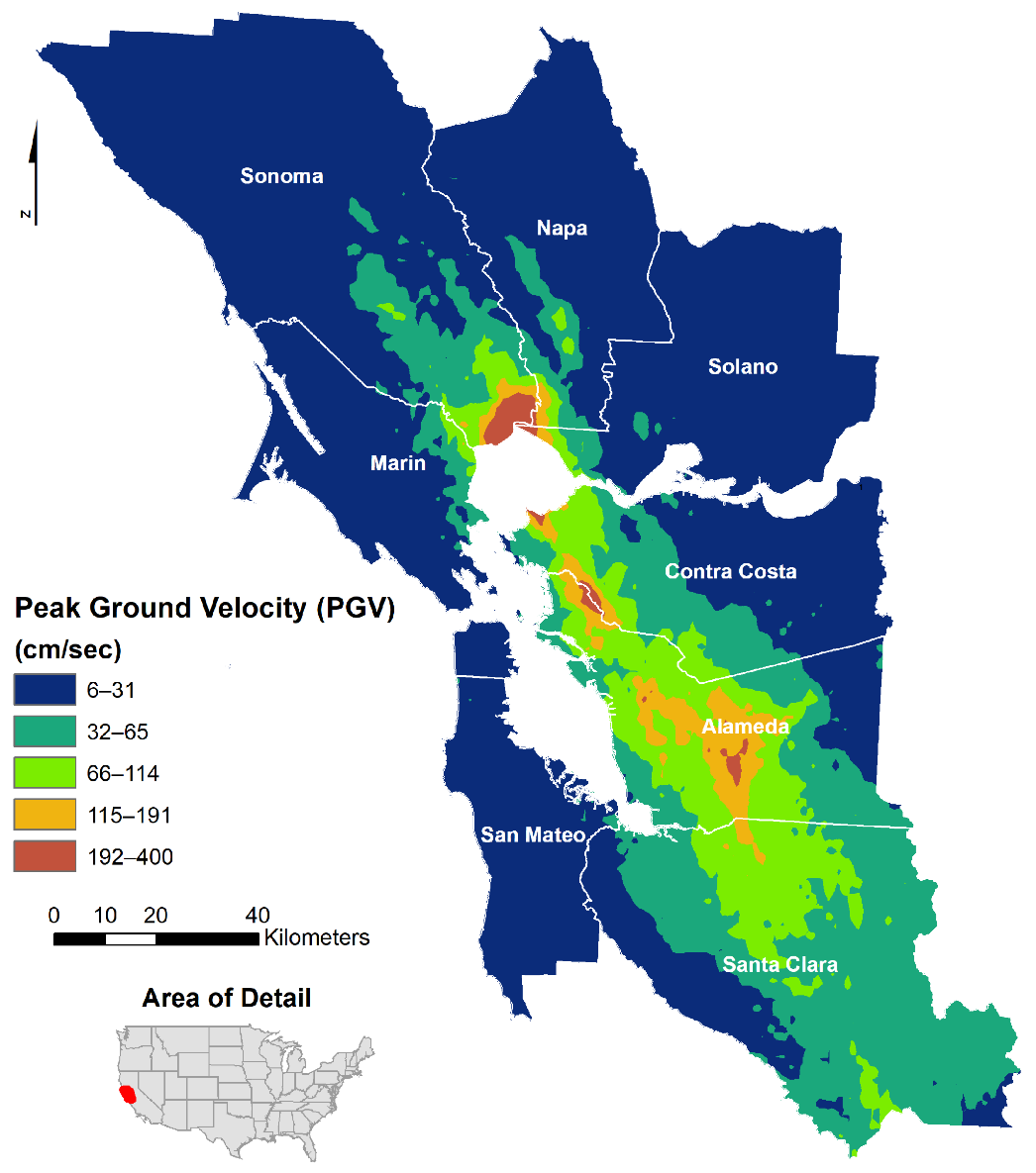
In the HayWired scenario, analysis of potable water supply was performed using the CUWNet water pipeline damage model in the East Bay Municipal Utility District (EBMUD) and San Jose Water Company (SJWC) service areas [1]. In Porter [1], the CUWNet model results included estimates of average water pipeline repairs (leak and breaks, per 1 km of pipe) made available by a ~90 m² (three-arcsecond) raster grid and summary reports of potable water service outage (hereafter, the above are referred to as the CUWNet model results). These service areas cover approximately 1.65 million people (615,000 service connections or households) or about 22% of the population in the nine counties adjacent to the San Francisco Bay (Alameda, Contra Costa, Marin, Napa, San Francisco, San Mateo, Santa Clara, Solano, and Sonoma Counties, in Figure 1—hereafter, the nine-county HayWired scenario study region, though this may include up to sixteen counties in other studies), which represents approximately 7.6 million people (2017 population estimate). Hazus (version 2.1) water system performance analysis was conducted by FEMA (Doug Bausch, formerly of FEMA Region VIII) for the rest of the HayWired scenario study region, using custom ground-motion data for the HayWired scenario mainshock [19].

In the case study, we extend applications of the CUWNet model to the nine-county HayWired scenario study region, using the simplified loss estimation approach to estimate water supply needs—without proprietary water pipeline data, and with increased precision.

The questions that arise are: (1) How does a simplified loss estimation approach for water pipeline damage compare with the CUWNet water pipeline damage model that uses proprietary infrastructure data? (2) What are the differences in regional estimates of household water service outage between the CUWNet model, the Hazus loss estimates and the simplified approach in the HayWired scenario? (3) What is lost and what is gained from higher precision estimates of emergency water resource requirements, used for rapid assessment, prioritization, and targeted allocation of emergency water resources?

To investigate these questions, we review the literature for analytical models of earthquake-induced pipeline damage and potable water service outages developed in previous efforts, with an emphasis on the Hazus loss estimation methodology [11] and the CUWNet water [1] pipeline damage model and its application in the HayWired scenario [18]. Using the brief literature review as a basis, we proposed a new simplified analytical method to estimate water supply needs in earthquakes.

In the simplified analytical method, Hazus water system performance analysis is adapted to use the new CUWNet water pipeline vulnerability function in Porter [1] to estimate average water pipeline break rates (per 1 km of pipe) by the ~90 m² (three-arcsecond) raster grid, in conjunction with water service outage calculated from the default Hazus serviceability index by the ~250 m² (nine-arcsecond) raster grid. The water pipeline vulnerability function is conditioned on hazard intensity data using peak ground velocities (PGV) and ground failure probabilities (e.g., liquefaction, landslides, and fault offset) from the HayWired scenario [19]. The LandScan USA 2017 “conus_night” (~90 m² at the equator, three-arcsecond) nighttime population database (hereafter referred to as the LandScan population database) [20] provides ambient population estimates in the model, for targeted emergency water resource allocation.

A sensitivity analysis of scale shows that the simplified method preserves the convex relationship between water pipeline damage and serviceability found in simulations of the hydraulic processes of the EBMUD water system [15] and is consistent with a level 1 Hazus water systems analysis, performed at the census tract scale study region [11]. Validation of the simplified method is performed in the EBMUD and SJWC study regions against the CUWNet model to estimate the accuracy and limitations of the approach applied in other areas.

In an emergency, the allocation of emergency drinking water to impacted populations may present significant challenges [3]. This study contributes new simplified methods to support the rapid estimation of emergency water demand for comprehensive planning and risk management in the event of a catastrophic earthquake [3,5]. Other models, such as the Hazus loss estimation methodology and CUWNet water system analysis, do not currently provide this level of precision in water service outage results—and may require proprietary inventory data, limiting their applications in no-notice earthquake events.

This study also contributes tools to address the societal implications of water service disruptions in vulnerable communities, where disproportionate impacts and hardships from potable-water service outages may lead to a greater need for emergency resources [6,7,8]. Developing methods for rapid assessment, prioritization and targeted allocation of emergency water resources could ensure resource access for the most vulnerable communities.

Future research is suggested to connect the methodology more closely with minimum emergency water supply needs rather than full water service restoration. General applications of the simplified method for estimating emergency water supply needs in earthquakes can be validated with further empirical studies.

2. Analytical Models of Water Supply Damage and Restoration

We review the literature for analytical models of earthquake-induced pipeline damage and potable water service outages developed in previous effort. The Hazus loss estimation methodology [11] and the CUWNet water pipeline damage model [1] are reviewed in detail.

Analytical approaches to estimating impacts to water-supply from an earthquake typically involve acquiring water-supply system inventory data, identifying component materials and sizes, and associating each with one or more vulnerability functions or fragility functions [1]. A vulnerability function relates the degree of damage, as in the case of damageability of buried pipe, to the number of breaks or leaks per unit length of pipeline as a function of the degree of ground-motion hazard intensity, such as peak ground velocity (PGV) and ground failure (e.g., landslide, fault rupture and liquefaction). Vulnerability functions are generally conditional on the pipeline’s engineering attributes (e.g., material, diameter, connections at joints) and sometimes on the soil conditions [1].

A vulnerability model can be deterministic, providing only a mean estimate of loss conditioned on ground motion and ground failure, or probabilistic, providing both a mean value and an estimate of uncertainty, in one or more scenario [1]. Repair costs and duration of loss of function (i.e., service outage) are then evaluated in serviceability models. Many authors have written extensively about the damageability of buried pipe—only some of this work, relevant to the current study, is discussed here.

The Hazus loss estimation methodology currently uses the O’Rourke and Ayala [21] vulnerability function (Equation (1)) conditioned on PGV (cm/sec) to estimate the median repairs per 1 km of pipe, or median repair rate (R) per census tract (from the U.S. Decennial Census geography) in a user-defined study region, with associated number of breaks and leaks in the water pipeline network.

$$R\left(PGV\right)=0.0001\times K\times PG{V}^{2.25}$$

(1)

$R$: median repair rate per 1 km of pipe;

K: ductility coefficient;

PGV: geometric mean horizontal peak ground velocity (cm/s).

A default Hazus water system analysis assumes 80% of water pipelines are cast iron, asbestos cement, or reinforced concrete cylinder (brittle pipes, with ductility coefficient, K = 1.0), with the remaining pipes assumed to be iron, steel, or polyvinyl chloride (ductile pipes, K = 0.3). Hazus uses the Honegger and Eguchi [22] vulnerability function (Equation (2)) to estimate the median number of repairs (breaks and leaks) subject to ground-failure, conditioned on Permanent Ground Displacement (PGD). PGD is a measure of the absolute distance a point on the ground permanently moves due to ground failure, in centimeters [1]. The probability of liquefaction is denoted as ($P_L$) in Equation (2), and (K) is the same as above.

$$R\left(PGD,P_L\right)=P_L\times K\times {(0.393701\times PGD)}^{0.56}$$

(2)

$R$: median repair rate per 1 km of pipe;

K: ductility coefficient;

PGD: permanent ground displacement (cm);

$P_L$: liquefaction probability.

Hazus is a nationally standardized methodology in the United States that contains models for estimating potential losses from earthquakes, floods, tsunamis, and hurricanes. Hazus uses Geographic Information Systems (GIS) technology and the U.S. Decennial Census geography to estimate physical, economic, and social impacts of disasters [11]. In the Hazus earthquake module, a user defined study region can consist of any combination of census tracts, from a single tract to those within an administrative/utility district or a broad regional area.

For an earthquake, a level 1 Hazus water system analysis produces the number of repairs (leaks and breaks) per 1 km of pipe in each census tract, using a default break-to-leak ratio. The median break rate per 1 km of pipe ($R_B$) per census tract is calculated, which is used in a serviceability index (discussed at the end of the section, below) to estimate the number of households in the study region with water service outage. In the level 1 Hazus water system analysis, potable water pipelines are assumed to exist under each street and the number of households in a census tract are assumed to be equivalent to the number of water service connections in the census tract [11]. Lengths of pipe are estimated as the total length of street centerlines within each census tract—without the use of water pipeline inventory data. A level 2 Hazus analysis can incorporate infrastructure inventory data, improved water pipeline vulnerability functions, and other user-supplied information [11].

More recently, O’Rourke et al. [23] developed vulnerability functions (Equation (3)) for the median repair rate per kilometer of asbestos cement or cast-iron pipes subjected to ground-motion hazard intensity. These vulnerability functions are based on empirical data from the M_w 6.2 February 22, 2011, Christchurch, New Zealand, earthquake, and the M_w 6.0 June 13, 2011, Christchurch earthquake. For pipe subjected to liquefaction, ground deformation is measured in terms of angular distortion—the permanent vertical displacement of two points on the pipe axis, divided by the distance between the two points [1].

$$R\left(PGV\right)=K_1\times lo{g}^p\left(PGV\right)\times {10}^{-5}$$

(3)

$R$: median repair rate per 1 km of pipe;

$K_1$: ductility coefficient: $K_1=1$ for asbestos cement, and $K_1=3.01995$ for cast iron pipes;

$PGV$: geometric mean horizontal peak ground velocity (cm/s);

p: exponent parameter: p = 0.83 for asbestos cement, and p = 2.38 for cast iron pipes.

The CUWNet model [1] for water pipeline repair rates uses the empirically based Eidinger [24] pipe vulnerability function for wave passage (ground-motion), rather than the Hazus vulnerability functions or O’Rourke et al. [23]. O’Rourke et al. [23] has been cited more often in the literature in far fewer years than Eidinger [24]. However, Eidinger [24] draws on a larger dataset and the vulnerability functions cover both ground-motion intensity and ground failure [1]. The Eidinger [24] pipe vulnerability function is based on 81 sources, identifying 3,350 repairs in 12 earthquakes, mostly from the M_w 6.7 1994 Northridge earthquake [1]. The average repair rate ($\overline{R}$) per 1 km of pipe from the Eidinger [24] pipe vulnerability function, with associated fractional number of breaks and leaks in the water pipeline network, is calculated in Equation (4), as:

$$\overline{R}\left(PGV\right)=K_1\times 0.003623\times PGV\times 0.393701\times 3.2808$$

(4)

$\overline{R}$: expected value or mean (average) repair rate per 1 km of pipe;

$K_1$: ground-motion ductility coefficient;

PGV: geometric mean horizontal peak ground velocity (cm/s).

Eidinger [24] proposed two vulnerability functions—one for wave passage (ground-motion) as in Equation (4), and one for PGD (with liquefaction or landslide-induced ground displacement), shown in Equation (5).

$$\overline{R}\left(PGD\right)=K_2\times 1.39\times \left(PGD\times 0.393701\right){ }^{0.319}\times 3.2808$$

(5)

$\overline{R}$: expected value or mean (average) repair rate per 1 km of pipe;

$K_2$: ground-failure ductility coefficient;

PGD: permanent ground displacement (cm).

In the CUWNet model, Porter [1] suggests a new vulnerability function, constrained by probability of liquefaction estimates (due to the absence of PGD information in the HayWired scenario) [1]. This new vulnerability function combines and simplifies the two Eidinger [24] vulnerability functions (Equations (4) and (5)) into one, assuming a moderate PGD associated with liquefaction probabilities from the HayWired scenario [1]. Ground failure ($P_L$) is denoted as the probability of occurrence of at least one type of ground failure (of liquefaction, landslide or fault rupture). Equation (6) for average breaks (${\overline{R}}_B)$ per 1 km of pipe with metric unit conversion results as:

$$\begin{array}{c}{\overline{R}}_B\left(PGV,P_L\right)=(\left(1-P_L\right)\times K_1\times 0.003623\times PGV\times 0.393701\times 0.15\\ +P_L\times K_2\times 2.46\times 0.5)\times 3.2808\end{array}$$

(6)

$\overline{R}$: expected value or mean (average) break rate per 1 km of pipe;

$P_L$: ground failure probability. We assume liquefaction, landslide and fault rupture are independent and model ground failure as: 1 − ((1 − liquefaction prob.) × (1 − landslide prob.) × (1 − fault rupture prob.));

$K_1$: ground-motion ductility coefficient;

$K_2$: ground-failure ductility coefficient;

PGV: geometric mean horizontal peak ground velocity (cm/s).

Hazard intensity is based on the simulated ground-motion PGV data from the HayWired scenario [19]. Porter [1] applies the break/leak ratio, identified by Ballantyne et al. [25], which found that pipeline damage from earthquake-induced ground-failure in several earthquakes resulted in a 50/50 percent break/leak ratio. In the absence of ground failure, the ratio was 15/85 percent breaks versus leaks. Liquefaction susceptibility in the San Francisco Bay Area [26] is used to estimate liquefaction probability [27], which is an extension of methods presented in Holzer et al. [28,29] for Santa Clara [28] and Alameda [29] Counties. Hazus loss estimation was used with liquefaction susceptibility maps [30] to estimate liquefaction probability in the rest of the study region [31]. Landslide probability [32] and fault rupture estimates [19] are from the HayWired scenario.

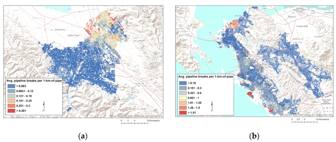
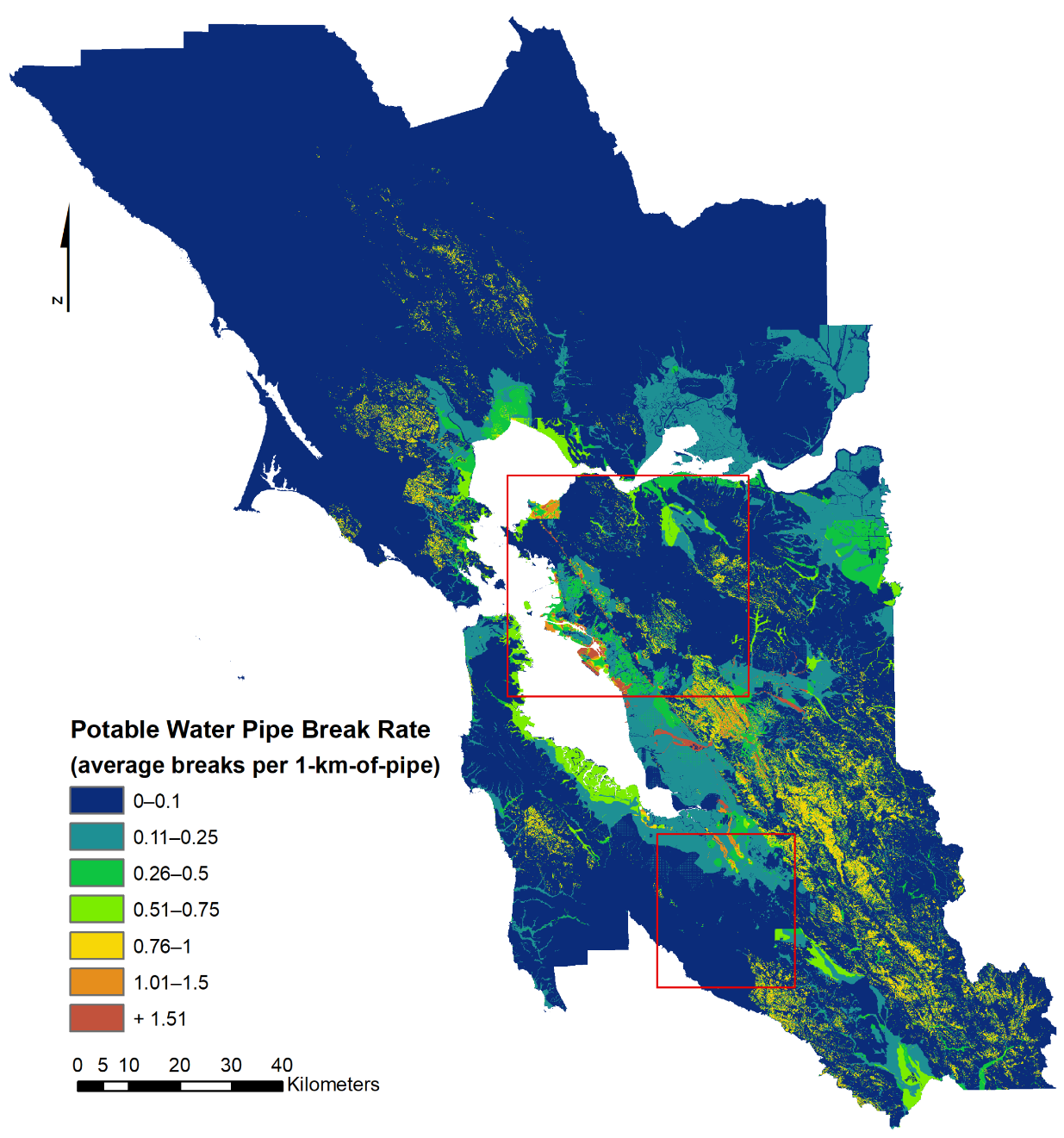
The average water pipeline breaks per 1 km of pipe (${\overline{R}}_B$) in the EBMUD and SJWC service areas for the HayWired mainshock are provided by the ~90 m² (three-arcsecond) grid centroid from Porter [1] in the CUWNet model results and are shown in Figure 2.

As demonstrated in [33], the CUWNet model focuses exclusively on buried pipe, which is where most water service restoration efforts are concentrated [1]. Recent developments have expanded the CUWNet model to include damage and repair to water pump stations [34]. Porter [1] applied the CUWNet model in the East Bay Municipal Utility District (EBMUD) and San Jose Water Company (SJWC) service areas for the HayWired scenario using proprietary water pipeline inventory data, and adjusted Hazus estimates for the rest of the nine-county study region.

The SJWC serves over 1 million people in most parts of the Cities of San Jose and Cupertino, and all of Saratoga, Los Gatos, and Campbell, including other small cities and unincorporated parts of Santa Clara County [1]. The 225,000 service connections, approximately one per household, entail an average daily demand for drinking water of roughly 120 million gallons, conveyed through 3,957.3 km of water pipes (mains). The EBMUD serves approximately 1.3 million people in Alameda County and Contra Costa County through 390,000 service connections (approximately one per household) [1]. Approximately one third of the EBMUD service connections are located east of the East Bay Hills, with the remainder in the lowlands between the hills and the San Francisco Bay, conveyed by gravity through 6,697.429 km of water pipes (mains). Both systems are subject to strong ground-motions in the HayWired scenario from mainshock and aftershock events [1].

How is water-supply serviceability estimated without a hydraulic model? Isoyama and Katayama [35] first proposed a measure called serviceability as the probability that the demand at a customer-service connection is fully satisfied, aggregated as the average number of customer-service connections in the entire system whose demand is fully satisfied [1]. Service outage can then be defined as the average number of customer-service connections in the entire system whose demand is not fully satisfied.

Markov et al. [36] proposed to measure serviceability using a serviceability index, defined by the ratio of total available flow to total required flow, which differs from the Isoyama and Katayama definition of serviceability. In the Hazus loss estimation [11], loss of serviceability is expressed as the percentage of “households without water” and is based on the Markov et al. [36] modeling of the EBMUD and San Francisco Auxiliary Water-Supply System and Isoyama and Katayama [35] modeling of Tokyo’s water-supply system. A simplified estimation of the potable water system network performance (i.e., number of households without water) uses the serviceability index, conditioned on the average water pipeline break rate per 1 km of pipe (${\overline{R}}_B$) within the user defined study region.

The default Hazus serviceability index [11] is modeled as an inverted log-normal cumulative distribution function of the mean break rate per 1 km of pipe (breaks, not leaks, per 1 km or 3280.84 linear feet of service main pipe) with parameters μ for median and β for logarithmic standard deviation in Equation (1).

$$1-S\left({\overline{R}}_B\right)=\mathsf{\Phi }\left(\frac{\ln \left(\frac{{\overline{R}}_B}{\mu }\right)}{\beta }\right):\mathrm{Water}\mathrm{Service}\mathrm{Outages}\mathrm{in}\mathrm{Hazus}$$

(7)

${\overline{R}}_B$: median, or mean (average) break rate per 1 km of pipe, by study area;

$S\left({\overline{R}}_B\right)$: serviceability index distribution;

μ: median parameter for serviceability index;

β: logarithmic standard deviation parameter for serviceability index;

$\mathsf{\Phi }(·)$: the standard normal cumulative distribution function.

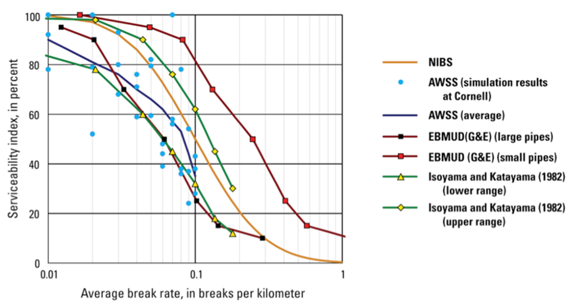
Hazus loss estimation employs parameter values of μ = 0.1 and β = 0.85, respectively, to generate the default serviceability index $S\left({\overline{R}}_B\right)$ for full water service restoration (from Equation (7), and National Institute of Building Science (NIBS), in Figure 3).

The CUWNet model in Porter [1] applies the default Hazus serviceability index $S\left({\overline{R}}_B\right)$ to estimate the fraction of services available immediately after the earthquake (at time, t = 0) in the HayWired scenario, by splitting the Eastern and Western portion of the EBMUD service area (using the East Bay Hills as the dividing line) and applying the serviceability index to each part. The proportional weighted percentage of available service connections (approximately equivalent to a household) was used to estimate the percentage of water service outages (at t = 0) for total system performance analysis.

The results of the CUWNet model shows that the SJWC can expect 1,054 repairs on average following the mainshock, of mostly small pipe damage (97%), occurring at a 28% to 72% break-to-leak ratio within the first day of the event (at t = 0). For the EBMUD, the CUWNet model estimates 4,294 repairs on average following the mainshock, of mostly small pipe damage (95%), occurring at a 37% to 63% break-to-leak ratio. The average EBMUD customer would be without water for six weeks and some customers could be without water service for up to seven months [1]. The average SJWC customer would be without service for only four days, as the SJWC service area is beyond areas of extreme ground motion. Alameda and Contra Costa Counties can expect about 71% of their households (in the EBMUD service area) to be without water service through the first week. After a month (at t = 30) this is expected to drop to about 46%, and after three months (at t = 90), 24% of households can expect continuing service outage. All water service restoration will be complete after seven months (at t = 210). A validation study of the CUWNET model in the 2014 Napa Earthquake suggests that the median model results may overestimate outages by about 10% [37]. See [1,33,34,37] for further discussion on these studies and the CUWNet model.

Recently, the Pacific Earthquake Engineering Research (PEER) center developed a hydraulic simulation (HydrauSim) model of water-supply system damage and applied it in a case study of the HayWired scenario, in the EBMUD service area [15]. The study found that the degree of total water shortages, on average, increased faster than the number of pipe failures—that is, the resulting total water shortage ratio trend was convex. This means that users in less-damaged regions could experience severe supply shortages regardless of local damage states, due to water path blockages from severely damaged regions further away [15].

These finding can be interpreted as evidence that in a simplified, deterministic approach, the convex relationship between the average water pipeline break rates (per 1 km of pipe) and serviceability may be dominated by the maximum (estimate of water pipeline damage, and service outage) within an analytical unit chosen to be consistent with simplified water system performance analysis tools such as Hazus or the CUWNet model.

In the Hazus earthquake module, a user defined study region can consist of any combination of census tracts, from a single tract to those within an administrative/utility district or within a broad regional area. The Hazus water system performance analysis is agnostic as to the choice of the study region— and the same default serviceability index is applied at various scales, depending on the study region. A minor to moderate loss of fidelity (or accuracy, for estimation purposes) results from the simplification of the hydraulic processes of the water system [38]. In this case, the Cross-Level (or “Ecological”) Inference Problem [39] arises when a water service outage is an outcome at the household level, but measurements are influenced by both the modifiable shape and scale of the aggregation unit, i.e., the analytical unit of the study region used in serviceability calculation. These issues cannot be avoided in simplified methods, but the loss of fidelity can be estimated—gains in precision can be made with the choice of an individual-level dasymetric population model.

The Bausch et al. [40] methodology was developed for the extension of Hazus loss estimation to international applications, e.g., [41,42,43]. The Bausch et al. [40] methodology uses the LandScan Global population database, with analysis performed by a ~1 km² (thirty-arcsecond) raster grid. LandScan Global 2017 and the LandScan USA 2017 “conus_night” (~90 m² at the equator, three arcsecond) population databases are products of Oakridge National Laboratories (ORNL), developed for emergency management applications [20]. The Landscan population database uses a dasymetric mapping technique to model ambient daytime and nighttime populations, based on the 2010 U.S. Decennial Census block populations and ancillary data (e.g., National Landcover Data (NLCD), water, diurnal population change) to expose the spatial distribution of the underlying population. LandScan population estimates are 95%, consistent with U.S. Decennial Census block population in heavily urban areas, and up to 99% in unpopulated areas [44]. The LandScan USA 2017 “conus_night” ~90 m² (three-arcsecond) population database [20] provides ambient nighttime population estimates in the model for targeted emergency water resource allocation.

3. Materials and Methods

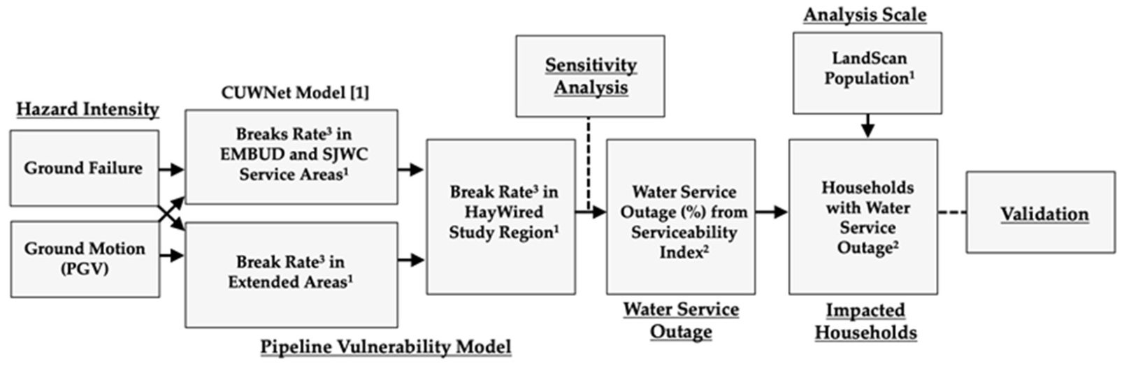
Using the brief literature review described above as a basis, we propose a simplified methodology for estimating water pipeline break rates and water service outage, which can be used for rapid estimation of emergency water supply needs after earthquakes. We illustrate the practical application of the simplified method through implementation in a case study of potable water service outage and emergency water requirements in the HayWired earthquake scenario. In general, there are seven stages to this methodology.

Earthquake-specific hazard intensity data are collected. In the case study, ground motion (e.g., PGV) and ground failure data (e.g., landslide, liquefaction and fault rupture) are provided from the HayWired Scenario [19].

A scale for analysis is selected. In the case study, data are mapped to the centroids of ~90 m² (three-arcsecond) raster grid cells used for analysis (which are identified as the $Cel{l}_{i,j}$) based on the scale of the LandScan population database [20].

A deterministic water pipeline vulnerability model is selected. In the case study, the CUWNet vulnerability function (Equation (6)) is applied directly to the ~90 m² (three-arcsecond) grid cell centroids (as discussed below, in Equation (8))—without the use of water pipeline inventory data. The vulnerability function is conditioned on the ground-motion (PGV) and ground failure probability at the centroid, to calculate the average break rate (${\overline{R}}_B$) per 1 km of pipe per ~90 m² (three-arcsecond) grid. In the case study, we include the Porter [1] ~90 m² (three-arcsecond) estimates of average water pipeline breaks per 1 km of pipe from the CUWNet model results within the EBMUD and SJWC service areas. The CUWNet model results are mapped to the $Cel{l}_{i,j}$ with a natural neighbor interpolation and then merged into a single feature class in Esri ArcGIS Desktop 10.7.1 replacing in the EBMUD and SJWC service areas, the results from the above calculations by Equation (8).

Sensitivity analysis is performed to select the appropriate analytical unit for serviceability calculations. Sensitivity analysis shows serviceability modeled by the maximum (percent) service outage per ~250-m² (nine-arcsecond) grid preserves the convex relationship between water pipeline damage and serviceability. This result is consistent with a level 1 Hazus water systems analysis performed at the census tract scale study region—and incurs a similar moderate loss of fidelity—but also provides a gain in precision.

Potable water service outages are estimated. The default Hazus serviceability index (Equation (7)) used in the CUWNet model, is applied in the case study with μ = 0.1 and β = 0.85 based on the NIBS curve in Figure 3. In the case study, potable water service outages (percent) are calculated per ~90 m² (three-arcsecond) grid cell centroid using the default Hazus serviceability index. The serviceability index result is taken to represent the average percent of households in each grid cell with full water services, as in the Hazus loss estimation methodology [11]. In a simplified, deterministic approach, the convex relationships between water pipeline damage and serviceability found in simulations of the hydraulic processes of the EBMUD water system [15] are modeled by the maximum (percent) service outage per ~250 m² (nine-arcsecond) grid cell—which includes nine underlying ~90 m² (three-arcsecond) raster grid cells, and their serviceability results.

Impacted households are estimated. In the case study, impacted households are estimated by a ~250 m² (nine-arcsecond) grid providing more precision in identifying the physical locations of impacted households with emergency needs in the San Francisco Bay Area. Populations from the LandScan USA 2017 “conus_night” (~90 m², three-arcsecond) nighttime population database are aggregated to the ~250 m² (nine-arcsecond) grid resolution—assuming the same population to household ratio as in the HayWired Scenario (~2.69 persons/household) [45]. Nighttime ambient populations are assumed to represent the location of household populations for analysis purposes.

The results are validated. In the case study, validation is performed by comparison with the CUWNet model results in the EBMUD and SJWC service areas to estimate the accuracy and limitations of the approach applied in other areas. These seven stages in the methodology (Figure 4, underlined) are presented below, as applied in the case study.

In the case study, the simplified method assumes that households, per ~250 m² (nine-arcsecond) grid cell, are equivalent to the service connections allocated to an unknown pipeline network in each grid cell that meets 100% pre-event flow for full-service capacity. This approach largely neglects the 15% or so of water service connections to nonresidential customers that would also be impacted, as further information on this relationship is unavailable.

The CUWNet vulnerability function [1] from Equation (6) was selected and adapted to calculate the average break rate (${\overline{R}}_B$) per 1 km of pipe by $Cel{l}_{i,j}$ centroids. Calculation of the average break rate (${\overline{R}}_B$) per 1 km of pipe performed at the grid cell centroid at this scale and without the use of any inventory data, is consistent with the level 1 Hazus loss estimation methodology [11]. In the case study, Equation (8) calculates the average break rate (${\overline{R}}_B$) per 1 km of pipe in areas outside of the EBMUD and SJWC service areas, with PGV in cm/sec, indexed by grid cell centroid ($i,j$):

$$\begin{array}{c}{\overline{R}}_B{}_{i,j}\left(PGV, P_L\right)=(\left(1-\left[P_L| Cel{l}_{i,j}\right]\right)\times K_1\times 0.003623\times \left[PGV|Cel{l}_{i,j}\right]\times 0.39370079\times 0.15\\ +2.46\times K_2\times [P_L| Cel{l}_{i,j}]\times 0.5)\times 3.2808\end{array}$$

(8)

${\overline{R}}_B{}_{i,j}$: expected value or mean (average) break rate per 1 km of pipe, per $Cel{l}_{i,j}$;

$P_L$: ground failure probability is estimated as the probability of occurrence for at least one type of ground failure (of liquefaction, landslide or fault rupture);

B = 0.15: Wave passage (ground-motion) component (break ratio), in the case study;

B = 0.5: Ground failure component (break ratio), in the case study;

$K_1$: ground-motion ductility coefficient;

$K_2$: ground-failure ductility coefficient;

$Cel{l}_{i,j}$: ~90 m² (three-arcsecond) raster grid cell, indexed by centroid ($i,j$);

i: latitude/northing (centroid);

j: longitude/easting (centroid);

[$P_L$|$Cel{l}_{i,j}$]: ground failure probability at the value of $Cel{l}_{i,j}$;

[PGV|$Cel{l}_{i,j}$]: peak ground velocity at the value of $Cel{l}_{i,j}$.

In the case study, the calculation applied the Ballantyne et al. [25] break-to-leak ratios (B) directly to the ground failure and wave passage parts of Equation (8). The values for $K_1$ = 0.69391934 and $K_2$ = 0.711281381 were taken from Porter [1] as the weighted average of the Eidinger [24] pipe-vulnerability equation ductility factors $K_1$ and $K_2$ for the EMBUD and SJWC study regions, found in Tables 1, 11 and 19 of Porter [1]. The choice for this parameter assumes that all areas in the HayWired study region have roughly the same age distribution for the underlying water pipeline infrastructure. This will underestimate damages in older communities and overestimate damages in newer communities, but a better estimate for this parameter is not available.

We assume that serviceability results are essentially unchanged between the initial event (t = 0) and three days after the event (t = 3) in the HayWired scenario, for the purpose of estimating water service outage and emergency water resource requirements by emergency managers. Emergency water resource requirements at three days after the event (t = 3) are estimated through the risk equation (Equation (9)), as adapted from the Office of the United Nations Disaster Relief Office (UNDRO) [46]. Results are aggregated across the nine-county HayWired study region. A resource multiplier of three liters of water per person per day is applied, assuming the same population to household ratio as in the HayWired scenario (~2.69 persons per household) [45].

$$Water Resource Requirements=Service Outage (\%)\times Population\times 3$$

(9)

The emergency water resource requirements can be aggregated to the Points of Distribution (PODS) sites that may support community water resource access in utility service areas, or Incident Command System (ICS) branch or division operational areas in mass care, humanitarian relief, and commodity missions in disaster response and response level exercises [2,47]. Planning for resource procurement of potable water supply by pallets of bottled water, truckloads, and bulk water tankers can be coordinated by private sector, government, and humanitarian relief organizations, in connection with the results, as a rapid assessment of emergency water resource needs.

4. Results

The simplified method to estimate water pipeline break rates, calculate potable water service outages and emergency water resource requirements was implemented in a case study of the HayWired scenario. The results in the nine-county HayWired scenario study region are presented below.

For the case study, hazard intensity data from the HayWired scenario included ground motion (e.g., PGV) and ground failure (e.g., landslide, liquefaction and fault rupture) data. For the analysis scale, the ~90 m² (three-arcsecond) raster grid cells were identified as the $Cel{l}_{i,j}$ based on the scale of the LandScan population database.

The average break rates per 1 km of pipe from the ~90 m² (three-arcsecond) grid cell centroids in the CUWNet model results from Porter [1] were mapped to the centroids of the $Cel{l}_{i,j}$ used in the current study, with a natural neighbor interpolation in Esri ArcGIS Desktop 10.7.1 (Figure 5). Areas within the bay, estuaries, or other unpopulated areas were removed, as they would not affect estimates of the impacted population.

The average break rate per 1 km of pipe was calculated using Equation (8) in the extended study region, by ~90 m² (three-arcsecond) raster grid, without water pipeline inventory data. These results were spatially merged with the CUWNet model results in the EBMUD and SJWC service areas into a single feature class in Esri ArcGIS Desktop 10.7.1 (Figure 6). The results show a continuous transition between the EBMUD and SJWC service areas and the extended areas.

A sensitivity analysis with various grid cell dimensions, numerical precisions and aggregation methods was performed in the EBMUD service area. The EBMUD service area was chosen for the sensitivity analysis as it is closest to the Hayward fault and will be more seriously damaged, with more local variation in hazard intensity. The sensitivity analysis ensured that the application of the serviceability index preserves the convex relationship between water pipeline damage and serviceability, and that the results are consistent with a level 1 Hazus water systems analysis, performed at the census tract scale study region—the smallest possible user defined study region.

First, using the CUWNet model results from Porter [1] to calculate serviceability in the EBMUD service area with the pipe lengths per 1 km-of pipe from the ~90 m² (three-arcsecond) grids, we verified that the Porter [1] result of 71% service outage (Record 11,

Table 1. Sensitivity analysis results for application of the serviceability index from CUWNet model results ¹.

Record	Unit	Model	Rounding 3	Outage (%) Calculation Input 4	Serviceability Calculation 5	Aggregation 6	Water Service Outage (%)	Water Service Outage (Pop 7)
1	250 m2 Grid	Simplified Approach 8	N/A	A	Local	Average 6	53%	543,417
2		Simplified Approach 8	N/A	A	Local	Maximum 6	59%	607,233
3		Weighted 9 Simplified Approach 8	N/A	A	Local	Weighted 9 Maximum 6	W 67% E 14%	607,233
							59%
4		CUWNet Model 10	Round	B	Global	None	68%	707,203
5		Weighted 9 CUWNet Model 10	No Round	C	Global	None	W 84% E 0.3%	738,310
							72%
6	200 m2 Grid	CUWNet Model 10	Round	B	Global	None	66%	672,794
7	500 m2 Grid						82%	835,012
8	1 km2 Grid						84%	855,896
9	Census Tract	CUWNet Model 10	Round	D	Local	None	61% 12	623,436
10			No Round	D	Local	None	61% 12	621,711
11	Study Region 11	Weighted 9 CUWNet Model 10	N/A	C	Global	None	71%	718,107

¹ Average break rates per 1 km of pipe and pipe lengths in EBMUD service area by ~90 m² grid cells in the CUWNet model results from Porter [1]. ² To avoid confusion, this is the usual exponent of the second power, as in $2^2=4$. ³ Rounding of breaks per unit (Avg. Break Rate ¹ × Pipe Length ¹). The breaks per total length of pipe per unit are rounded or not rounded for input in the serviceability calculation ⁴. This can only occur if water pipeline inventory data is available. ⁴ A = Average break rates ¹; B = Global ⁵ average of unit break rate, calculated by breaks per unit ³ divided by total pipe length per unit; C = Weighted ⁹ average of unit break rate, calculated by breaks per unit ³ divided by total pipe length per unit; D = Unit break rates calculated by breaks per unit ³ divided by total pipe length per unit. ⁵ Serviceability and outage (%) calculated at the local—by grid cell unit—or global—by EBMUD study region as: Outage (%) = 1 − Serviceability (%). ⁶ Average of unit outages (%) or Maximum of unit outages (%) from serviceability calculation ⁵ by ~90 m² grid cells. ⁷ Population from LandScan USA 2017 estimates used for both CUWNet model and simplified approach in this analysis. ⁸ Simplified Approach: Calculated without the use of inventory data (i.e., pipe lengths ¹). Serviceability calculated per ~90 m² grid cell as a function of the average break rate ¹ and aggregated in the serviceability calculation ⁵ per unit. ⁹ Weighted: Eastern (E) and Western (W) EBMUD outage calculated separately and proportionally weighted by (%) population in the simplified approach or CUWNet model and by service connections in Porter [1]. ¹⁰ CUWNet Model: Calculated with the use of inventory data (i.e., pipe lengths ¹) and by breaks per unit ³. ¹¹ Western and Eastern EBMUD study region. ¹² Equivalent to a Hazus loss estimation global result at the census tract scale study region with Porter [1] vulnerability function.

) could be closely replicated by weighting Eastern and Western EBMUD regions by the percent of population from the LandScan population database [20]. Porter [1] originally performed the weighting by service connections—assuming one third of the service connections were located east of the East Bay Hills (eastern), with the remainder in the lowlands between the hills and the San Francisco Bay (western). In Record 5 of Table 1, we found 72% service outage with the new approach—which held for any grid resolution, as there is no round-off error in the CUWNet method.

We proceeded to change the grid unit dimensions (e.g., ~90 m², ~200 m², ~250 m², ~500 m², and ~1 km²) and rounded the breaks calculated per unit to determine the average break rate in the study region. We slightly modified the CUWNet model to align with the Hazus approach, as the Hazus Technical Manual [11] indicated that breaks are rounded per unit (i.e., pipes either break or they do not, there are no fractional breaks)—while the CUWNet model does not round breaks per unit (and so there is no round-off error). Service outage was estimated with a global serviceability calculation at the EBMUD service area scale, rather than with a weighted global approach. Serviceability in a global approach or a weighted global approach provide essentially the same result if the percentages are the same—both approaches will result in the same percentage of population in the user defined study region with service outage.

In Records 6—8, the percent with service outage fluctuated, but was closest (Record 4) to 71% (the benchmark estimate from Record 11) only when the grid unit dimension was ~250 m² (nine-arcsecond). These fluctuations were caused by round-off error in calculating the breaks per unit—as when there are more grid cells (i.e., smaller dimensions) there are more opportunities for rounding, and vice versa. In Record 4, we found that the closest possible global result is 68%—about a 4% loss of accuracy in comparison with the 71% benchmark service outage estimate. Loss of accuracy was calculated as percent change (decrease or increase) by Equation (10):

$$\frac{\left(V_2-V_1\right) }{\left|V_1\right|}\times 100$$

(10)

$V_1$: starting percentage;

$V_2$: comparison percentage.

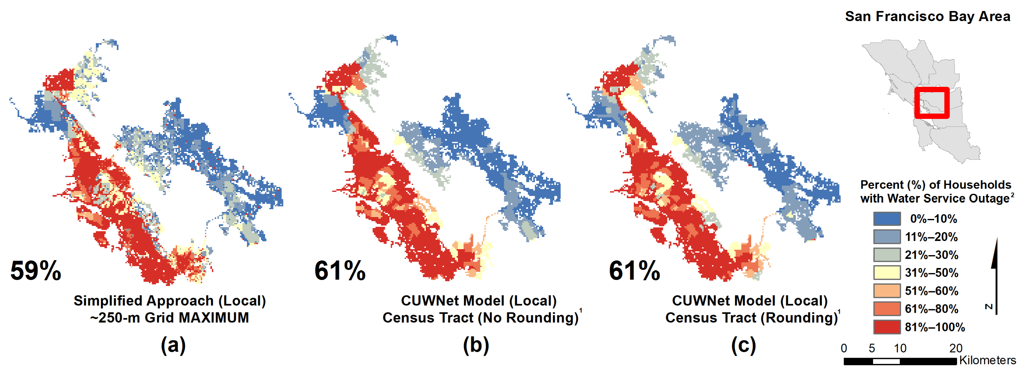
We then estimated the loss of fidelity in the local, simplified approach by ~250 m² grid cell unit through a direct comparison with a global service outage estimate in the EBMUD service area. Different aggregation methods were tested (Records 1—2), but only the maximum service outage of the nine underlying ~90 m² (three-arcsecond) grid cells in the ~250 m² (nine-arcsecond) grid cell unit conserved the convex relationship between water pipeline damage and serviceability in the simplification of the hydraulic processes of the water system, per unit. In Records 2—3, both the weighted and unweighted local approach to serviceability calculation resulted in 59% service outage—about a 13% decrease from 68% (Record 4), sacrificing some accuracy in the system performance estimates from the global approach for more precision in the estimates of the location of service outages with the local, simplified approach.

To ensure that application of the serviceability index was consistent with the results of a Hazus water systems analysis result performed at the census tract scale study region, we applied the CUWNet model by census tract with the local serviceability approach. This was like running a Hazus water system analysis (replacing the default Hazus water pipeline vulnerability function in Equation (1), with Equation (6)) with the global serviceability approach for each user-defined census tract study region and then aggregating the results across the EBMUD service area—a common method in Hazus loss estimation for combining multiple study regions [11]. The result with both rounded and not rounded breaks per census tract was 61% service outage, in Records 9—10 (i.e., the method was not sensitive to numerical precision of breaks at that scale). The small difference between 59% and 61% indicated that our method was sound (about 3% difference), and at the lower range of what a Hazus loss estimate might produce. The key results from the sensitivity analysis are presented below in Table 1 and mapped in Figure 7.

The loss of fidelity in the simplified approach compared with the CUWNet model results in Porter [1] of 71% was an overall decrease of about 17% in the EBMUD service area. This decrease was roughly equivalent to the minor to moderate loss of fidelity introduced in a level 1 Hazus water system analysis estimate of global service outage at the census tract scale study region. The moderate loss of fidelity results from simplification of the hydraulic processes of the water systems [38].

The serviceability index (Equation (7)) with the parameter values of μ = 0.1 and β = 0.85, conditioned on the spatially merged average break rate per 1 km of pipe (${\overline{R}}_B$), was calculated per ~90 m² (three-arcsecond) grid cell. The maximum (percent) service outage per ~250 m² (nine-arcsecond) grid is selected and mapped in Figure 8 to estimate the percent of households with water service outages (at t = 0). Many areas in the results have the potential for extensive serviceability impacts, but little or no population.

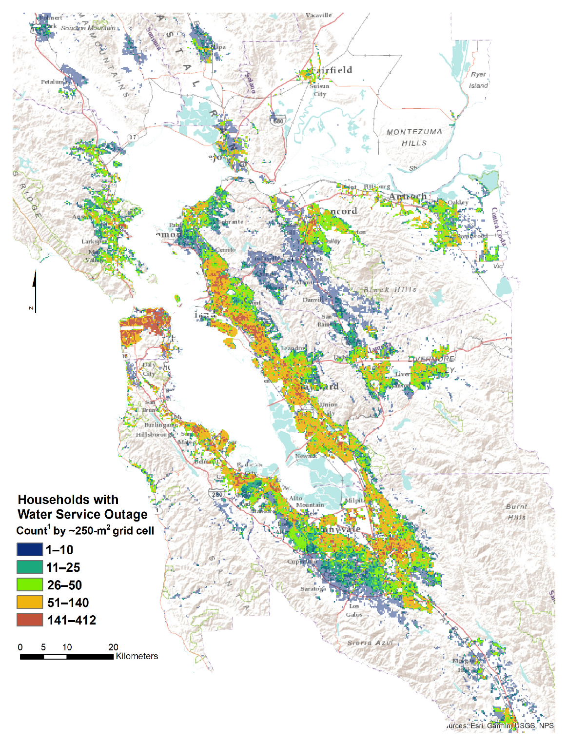
An estimate of households (and residents) with potable water service outage in the HayWired scenario was calculated through the risk equation (Equation (9)) and mapped in Figure 9, throughout the nine-county HayWired study region. Expanding estimates of water pipeline break rates and potable water service outages identified additional areas (

Table 2. Summary of results in the nine-county HayWired scenario study region.

County	Households (2017)	Water Service Outage (%)	Water Service Outage (HH) 1	Minimum Emergency Requirements 4 (%)	Minimum Emergency Requirements 4 (HH) 1	CUWNet Water Service Outage (%)	(Adjusted 2) Hazus Water Service Outage (%)	(Adjusted 2) Hazus Water Service Outage (HH) 1
Alameda	609,349	81%	490,690	51%	312,249	71% 3	71%	432,638
Contra Costa	416,943	39%	164,654	22%	93,179		71%	296,030
Marin	93,945	65%	61,210	47%	44,348	N/A	6%	5637
Napa	51,543	14%	7420	6%	3063	N/A	0%	0
San Francisco	322,445	48%	156,171	29%	94,822	N/A	45%	145,100
San Mateo	282,786	48%	135,723	33%	94,512	N/A	64%	180,983
Santa Clara	715,266	47%	334,382	21%	153,003	33% 3	30%	214,580
Solano	161,145	15%	24,850	9%	14,293	N/A	1%	1611
Sonoma	182,983	3%	6274	1%	1514	N/A	0%	0
Total	2,836,295	49%	1,381,374	29%	810,985	N/A	45%	1,276,570

¹ Households estimated using population from LandScan USA 2017 “conus_night” with approximately 2.69 persons per household (HH). ² Adjusted HAZUS estimates from Table 30 in Porter [1]. ³ In the EBMUD service area and SJWC service areas, respectively. ⁴ From the discussion in Section 5.

) in Fremont (Alameda County) and the eastern part of San Jose (Santa Clara County), along with areas in eastern Alameda and Contra Costa Counties, Marin County, San Mateo County and San Francisco with potential emergency water resource requirements that were not originally identifiable in the HayWired CUWNet analysis.

The simplified approach estimated about 1.38 million households (3.7 million residents) out of 7.6 million residents (2017 population estimate) with potable water service outage in the nine-county HayWired study region, three days after the event (t = 3). The (t = 3) estimated emergency water requirements total about 9 million liters of water needed.

Validation and Comparisons in EBMUD and SJWC Service Areas

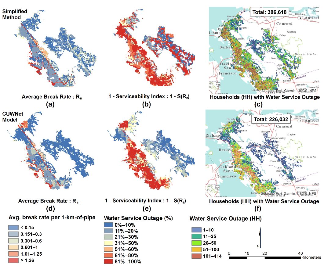
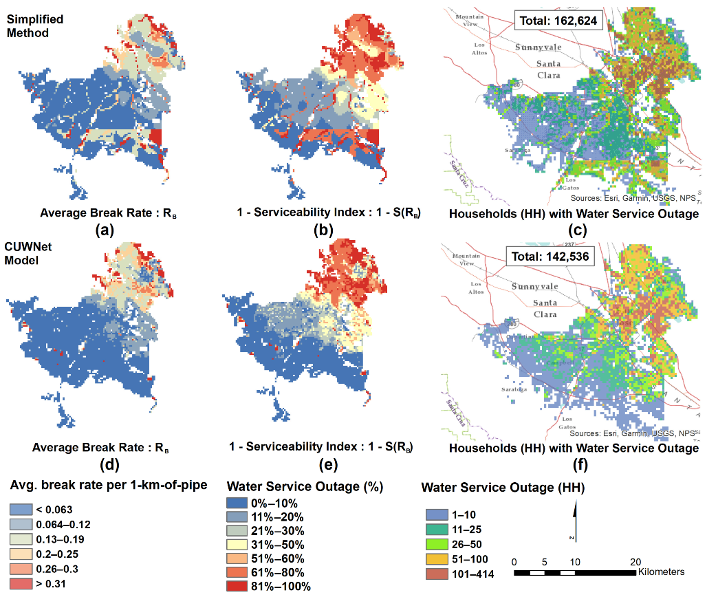
Study validation is performed by comparison of the simplified method with the CUWNet model results in the EBMUD and SJWC areas to estimate the accuracy and limitations of the approach applied in the rest of the study region. Estimates of households with full water service outage calculated from the maximum (percent) service outage within the ~250 m² (nine-arcsecond) grid cells using the CUWNet model results are compared with the simplified approach applied in the same EBMUD and SJWC service areas.

In the EBMUD service area, the estimates of households with full water service outage from the CUWNet model results [1] for the average break rates per 1 km of pipe show about 226,032 households (607,233 residents) or about 59% of the total population in the service area (from Table 1, Record 2). For comparison, the simplified approach shows about 386,618 households (1,033,273 residents) with water service outage, or about 70% of the total population in the same EBMUD service area.

The simplified approach moderately increased estimates of households with water service outage in dense urban areas, exposed to high hazard intensities near the fault. In areas of Contra Costa County, the CUWNet model used a proportional estimate of liquefaction from Alameda County, while the simplified approach used the Hazus estimates of liquefaction probability in Contra Costa County [18]. This resulted in an underestimation of break rates by the CUWNet model in Porter [1] in these areas and accounts for most of the difference in comparison. Porter [1] also shows less pipeline inventory in many areas with high liquefaction hazard. The simplified approach may increase estimates in these areas. Ground-motion intensities change rapidly over smaller areas near the fault, and so inventory data used in calculating breaks in the CUWNet model for the average break rates per 1 km of pipe will provide a more accurate estimate in dense urban areas (Figure 10). The simplified approach may provide a reasonable estimate of households with water resource needs in areas near the fault, if detailed studies are unavailable. This conclusion is further discussed, in the following section, in comparison with other study results.

In the SJWC service area, the estimates of households with full water service outage from the CUWNet model break rate data show about 142,536 households (382,923 residents) or about 38% of the total population in the service area. For comparison, the simplified approach shows about 162,624 households (436,888 residents) with water service outage, or about 43% of the total population in the same SJWC service area (Figure 11).

Ground-motion intensities decrease and change less frequently over larger areas further from the fault. Therefore, detailed inventory data may not make as much of a difference in the break rate calculations in comparison with break rates from the CUWNet model results. Differences in comparison are limited to a few random dense urban areas. The Hazus estimates of liquefaction probability in Santa Clara County [31] lead to higher estimates of break rates in the southern part of the SJWC service area in the simplified approach. These estimates of liquefaction were not used in the CUWNet model, and likely account for most of the differences in the comparison. These results provide evidence for validation that the simplified approach may accurately represent water service outages in many of the areas further from the fault, throughout the nine-county HayWired study region.

5. Discussion

The simplified analytical method to estimate water supply needs in earthquakes is discussed below. The results of the case study in the HayWired scenario are discussed in context and comparison with similar studies performed in the nine-county San Francisco Bay Area, California (USA) study region. We revisit the three questions proposed in the introduction, to gauge its performance. Limitations of the simplified method are investigated, and the theoretical and practical implications of the results are suggested. Future research is proposed to connect the methodology more closely with minimum emergency water supply needs, with further validation of the model in general applications.

How does the simplified method compare with the CUWNet water pipeline damage model that uses proprietary infrastructure data? Proprietary infrastructure data would seem to be a prima facie condition for estimating water supply needs through water pipeline damage vulnerability functions in earthquakes—this may not be the case. The validation study with the CUWNet model results shows that the simplified method may accurately represent water service outages in many of the areas further from the fault, throughout the nine-county study region and provides a reasonable estimate in areas near the fault, if detailed studies are unavailable.

Many simplified methods assume that water pipelines can be replaced by street centerlines, e.g., [11,48]. However, when the research aim is to estimate water supply needs—rather than water pipeline damage and repair—we need only focus on the population that is impacted. A high resolution dasymetric population estimate can replace the assumption that service connections (as households) are allocated to the total length of pipe (or street centerlines, by proxy) aggregated within the analytical unit (census tracts, in Hazus loss estimation and the ~250 m² (nine-arcsecond) grid cell in the current study). Our results show that we need only know the average break rate per 1 km of pipe per analytical unit, and an estimate of the total number of households to calculate water service outage—the actual lengths of pipeline within the unit are not pertinent to our goal. We have gained the knowledge that a simplified analytical method for estimating water supply needs can be performed without proprietary water pipeline infrastructure data.

What are the differences in regional estimates of household water service outage between the CUWNet model, the Hazus loss estimates and the simplified approach in the HayWired scenario? In the validation study, we found that the simplified method increased estimates of households with water service outage by about 70% in comparison with the CUWNet model. Local variation in hazard intensity, the differences in ground-failure datasets used in analysis between the two methods, and the 17% loss of fidelity in the simplified approach make the assessment of these differences difficult in areas near the fault. The CUWNet model may underestimate household water service outage in the Cities of Richmond, CA (pop. 108K), El Cerrito, CA (pop. 25K) and San Pablo, CA (pop. 31K) based on the choice of ground-failure estimates for Contra Costa County in Porter [1]. The CUWNet model may also overestimate median service outages by about 10% [37]. In the validation study, the simplified approach estimated 70% (not to be confused with the 70% increase above) of the households in the EBMUD study region with water service outage, which is actually very close to the 71% reported in Porter [1] with that method and the CUWNet model, though that number may be too low.

In the HydrauSim model and case study in the HayWired scenario [15], about 25% of the demand nodes on average (i.e., service connections) may experience water shortages—which can rise to 78% for the worst-case scenario. This range of estimates from hydraulic modeling in the EBMUD service area includes both the CUWNet model and simplified method results as possible outcomes, even accounting for the 17% loss of fidelity in the simplified approach. This evidence validates that the simplified method provides a reasonable estimate of households with water service outages in areas near the fault, if detailed studies are unavailable.

In areas further from the fault, our results show that the simplified method overestimated households with service outage from the CUWNet model by about 12%, which is mostly due to the choice of ground-failure data. Other than that limitation, the results from the validation study provide evidence that the simplified approach may accurately represent water supply needs in many of the areas further from the fault.

The adjusted Hazus results from the HayWired scenario provide the best estimate of water service outage for comparison with the simplified method in the nine-county study region. The adjusted Hazus results (in Table 30 of Porter [1]) show approximately 1,276,575 total households (from LandScan USA 2017 nighttime, population estimates) with water service outage across the study region in the HayWired scenario, three days after the event. These results are summarized in Table 2 as the percent (%) of households with potable water service outage by county. For comparison, the simplified method estimates 1,381,374 households with water service outage in the study region. These results are also summarized in Table 2—with a modest 8% increase over the HayWired scenario.

In areas, such as Marin, Napa, Solano, and Sonoma Counties, increases in households with water service outage are shown (increases from 6% to 65% in Marin, 0% to 14% in Napa, and 1% to 15% in Solano Counties). Including ground failure in the simplified approach, by the ~90 m² (three-arcsecond) grid, accounts for much of this increase, as liquefaction occurs in populated areas—and may contribute to more accurate estimates. The low 39% Contra Costa County estimates from the discussion above are also shown in Table 2.

The simplified method estimates by ~250 m² (nine-arcsecond) grid represents the physical location of households that may experience service outages and emergency water resource requirements with far more precision than those provided by adjusted Hazus county summary information—or any other simplified analytical method, though there is a moderate loss of fidelity in the results. In consideration of this, it is important to identify the limitations of the model.

What is lost and what is gained from higher precision estimates of emergency water resource requirements? We investigate the 17% loss of fidelity in the simplified approach when applied in the EBMUD service area, in comparison with the CUWNet model results. One important theoretical limitation of the HayWired scenario, and scenario-based approaches in general, is that they only depict a single realization of fault rupture, ground motion, and other parameters—they provide models that resemble ground shaking in real earthquakes, though an actual event will certainty happen differently [19].

For a more robust calculation of the loss of fidelity in the simplified method, a regional risk assessment approach by probabilistic seismic hazard analysis (PSHA) can be implemented to produce various ground-motion scenarios, as in the HydrauSim modeling [15]. The loss of fidelity can be calculated with multiple simulations of ground motion applied in the simplified method, compared with the average realization of ground-motion and uncertainty can be quantified in the loss of fidelity estimate. Without a robust estimate of the loss of fidelity, we must use the maximum 17% loss estimate in the EBMUD service area and extrapolate it within the HayWired scenario (which is also close to the worst-case scenario estimate from the hydraulic modeling studies). This estimate is the best available measure of how well the simplified method performs in comparison with a global approach like the CUWNet model. This assumption remains a limitation.

In the simplified method, we have gained precision estimates of the locations of households with water service outage—when before, there were none. This knowledge allows for the rapid estimation of emergency water demand for comprehensive planning and risk management in humanitarian relief missions. The simplified method contributes tools for rapid assessment, prioritization, and targeted allocation of emergency water resources. The disproportionate impacts of utility service outage and excessive hardship experienced by some households can be mitigated if resource access is prioritized for the most vulnerable communities—an important practical implication of the model’s application. Substantial gains in utility from precision estimates of short-term emergency water resource needs for management of humanitarian relief missions may offset theoretical losses in accuracy, in practical application.

The model has other limitations. The CUWNet vulnerability model (Equation (6)) is tailored to the HayWired Scenario, by assuming a moderate PGD associated with liquefaction probabilities from the scenario. The ductility coefficients in Equation (8) are also based on the assumption that all areas in the HayWired study region have roughly the same average age distribution as the EMBUD and SJWC for the underlying water pipeline infrastructure. For more general application of the simplified method, other vulnerability functions must be applied, based on the maximum PGV in the scenario or earthquake event with general parameters for ductility. Further investigation with the O’Rourke and Ayala [21] and Honegger and Eguchi [22] vulnerability functions could make the simplified method directly compatible with the current Hazus loss estimation methodology. As the simplified method does not require proprietary infrastructure data, it could theoretically be implemented for any general earthquake application that the Hazus loss estimation methodology is currently used for, which includes all strike-slip/transform, normal, reverse/thrust fault types in the United States, and custom international applications. General applications of the simplified method for estimating emergency water supply needs in earthquakes can be validated with further empirical studies and the model can be calibrated with reconnaissance data from previous events, such as the 2014 Napa Earthquake.

Future Research on Minimum Emergency Water Supply Needs, Household Displacement and Modeling Humanitarian Relief

In the HayWired scenario, Porter [1] identified that the default Hazus serviceability index may need to be investigated and replaced, and that serviceability could be reformulated to estimate a minimal flow for emergency needs, rather than full restoration of water services. A recent validation study of the Porter [1] model in the 2014 Napa Earthquake suggests that the median model results may overestimate outages by about 10%, motivating further investigation of serviceability [37]. The CUWNet model results also indicate a majority (95–97%) of damage occurs to small pipes [1].

Modifying the default Hazus serviceability index parameters (to μ = 0.25 and β = 0.85) based on a theoretical curve fitting the empirical data from EBMUD for the serviceability of small pipes (G&E, in Figure 3) may be a first step in future research on this reformulation. The modified serviceability index decreases the impacted population by about 52% (in Table 2) but connects the methodology more closely with minimum emergency water resource needs (rather than full water service restoration). Results using the modified serviceability index may include private household water service-line connections (small pipes) that contribute to household service outage—damages that are not within the scope of repairs made to water utility pipeline networks.

In the nine-county HayWired study region, the modified serviceability index hypothetically estimates 810,985 households (2,178,706 residents) with 6,536,117 liters of emergency bottled water required to meet minimal needs, three days after the event. The minimum emergency water resource requirements are summarized in Table 2. These estimates are also aligned with the expert opinion from the Bay Area Earthquake Plan [47] for emergency commodity distribution. The Bay Area Earthquake Plan estimates a mass care mission supporting food for approximately 650,000 households (1.75 million people) and potable water for 5 million residents (about half receiving bottled water, and half receiving bulk water) three days after a similar earthquake event [2,47]. Expanded research for selection, validation, and calibration of the parameter μ in the serviceability index may relate water pipeline break rates to the fraction of customers not receiving minimal thresholds of flow for emergency drinking, cooking, and sanitary needs.

Additional uncertainty from the estimation of household structure, short-term evacuations and population displacement may increase or decrease emergency water resource requirements in areas throughout the study region, with household displacement expected at between 6–10%, based on the HayWired scenario estimates [45]. The model assumes that ambient nighttime populations from the LandScan USA 2017 “conus_night” population database can represent the location of households for analysis purposes. However, LandScan is an ambient population count—the values represent the average estimate of people who could be present in an individual cell during the nighttime. While this estimate will mostly include households, based on the diurnal population cycle and sleep behaviors, it is not confined solely to residences (e.g., bars and nightclubs may stay open until 2–3:00 AM; some grocery, restaurants and convenience stores are open 24 h). An individual-level population model, or population synthesis method [49] could provide a more robust estimate of household structure within the study region. The simplified method also largely neglects the 15% or so of water service connections to nonresidential customers that could be impacted, assuming instead that all service connections are households. Further applications of short-term displacement modification factors and more refined household estimates in future research may account for some uncertainty in the location of households, when estimating emergency water resource requirements.

The applications of the model can be expanded to include estimates of emergency food as well as water resource requirements in an earthquake, similar to those identified in the Bay Area Earthquake Plan [47]. Damage to lifeline infrastructure systems such as electric power, gas and water pipelines, bridges, roads, and railways, all affect the availability of food and water in a disaster. The percent of households impacted by utility service outage and transportation disruption could be weighted by a measure of the socioeconomic and demographic characteristics that contribute to risk disparity for post-disaster food insecurity and resource access experienced by individual households [50]. These estimates could be used to rapidly allocate emergency food and water resources—in a broader conceptual modeling framework—that could include the results of the current study.

6. Conclusions

This study developed a new simplified analytical method to estimate water supply needs in earthquakes, and extended applications of the CUWNet model in a case study of the HayWired earthquake scenario in the nine counties adjacent to San Francisco Bay in California (USA). The simplified loss estimation approach—performed without proprietary data—provided precision estimates of water pipeline break rates and household water service outage. Validation with the CUWNet model results showed that the simplified method may accurately represent water service outages in many of the areas further from the fault, throughout the nine-county study region and provides a reasonable estimate in areas near the fault, if detailed studies are unavailable.

We found that the 17% loss of fidelity in the simplified approach (compared to the CUWNet model in the EBMUD service area) was roughly equivalent to the minor to moderate loss of fidelity introduced in a level 1 Hazus water system analysis at the census tract scale study region—which results from simplification of the hydraulic processes of the water systems. The simplified approach sacrificed some accuracy in the water system performance estimates for more precision in the estimates of the location of service outages and emergency water supply need—which current loss estimation methods are often unable to identify.

These high-resolution spatial estimates of emergency water resource demand areas could assist emergency managers in mass care and emergency water commodity missions in response to and exercise of a M_w 7.0 Hayward Fault earthquake like the HayWired scenario. Simplified methods to estimate the location of emergency water supply need could provide the practical research advancement that would allow emergency managers to rapidly prioritize and allocate emergency water resources to the most severely impacted areas.