Article

Mapping Risk to Land Subsidence: Developing a Two-Level Modeling Strategy by Combining Multi-Criteria Decision-Making and Artificial Intelligence Techniques

1
Department of Earth Sciences, Faculty of Natural Sciences, University of Tabriz, 29 Bahman Boulevard, Tabriz 5166616471, East Azerbaijan, Iran
2
Institute of Environment, University of Tabriz, Tabriz 5166616471, East Azerbaijan, Iran
3
Traditional Medicine and Hydrotherapy Research Center, Ardabil University of Medical Sciences, Ardabil 5618985991, Ardabil, Iran
4
Department of Civil Engineering, University of Maragheh, Maragheh 5518183111, East Azerbaijan, Iran
5
Department of Bioresource Engineering, McGill University, 21111 Lakeshore, Ste Anne de Bellevue, QC H9X 3V9, Canada
6
Department of Geography & Environmental Studies, Wilfrid Laurier University, Waterloo, ON N2L 3C5, Canada
*
Author to whom correspondence should be addressed.
Water 2021, 13(19), 2622; https://doi.org/10.3390/w13192622
Submission received: 13 August 2021 / Revised: 6 September 2021 / Accepted: 16 September 2021 / Published: 23 September 2021

Abstract

:
Groundwater over-abstraction may cause land subsidence (LS), and the LS mapping suffers the subjectivity associated with expert judgment. The paper seeks to reduce the subjectivity associated with the hazard, vulnerability, and risk mapping by formulating an inclusive multiple modeling (IMM), which combines two common approaches of multi-criteria decision-making (MCDM) at Level 1 and artificial intelligence (AI) at Level 2. Fuzzy catastrophe scheme (FCS) is used as MCDM, and support vector machine (SVM) is employed as AI. The developed methodology is applied in Iran’s Tasuj plain, which has experienced groundwater depletion. The result highlights hotspots within the study area in terms of hazard, vulnerability, and risk. According to the receiver operating characteristic and the area under curve (AUC), significant signals are identified at both levels; however, IMM increases the modeling performance from Level 1 to Level 2, as a result of its multiple modeling capabilities. In addition, the AUC values indicate that LS in the study area is caused by intrinsic vulnerability rather than man-made hazards. Still, the hazard plays the triggering role in the risk realization.

1. Introduction

Land subsidence (LS) due to groundwater over-abstraction is a man-made problem, which threatens water availability, the environment, and structures. Risk assessment, as the first step of risk management, can play a pivotal role in proactively managing or mitigating LS problems. Risk assessment can be carried out by risk indexing or mapping when historical records are unavailable, and, consequently, frequency analysis is not feasible. Different techniques are available in the ongoing research activities to formulate risk indexing or mapping by incorporating a set of data layers, as discussed in due course. However, they suffer from subjectivity associated with the data layers due to expert judgment. The paper aims to delineate risk maps to LS and reduce the subjectivity by incorporating multi-criteria decision-making (MCDM) and artificial intelligence (AI) techniques, two widely used approaches in hydrology and environmental studies.
The literature review highlights two different approaches of MCDM and AI in risk mapping of groundwater issues. MCDM formulates the issue as a decision-making problem and aims to estimate the weights of different criteria in a pre-defined procedure. Various issues are available in the literature that are studied by the MCDM technique, including groundwater vulnerability to pollution by analytic hierarchy process (AHP) [1] and analytic network process (ANP) [2], groundwater potential indexing by multi-criteria decision analysis (MCDA) [3], and fuzzy catastrophe scheme (FCS) [4], groundwater risk to saltwater intrusion by FCS [5], and LS problem by FCS [6]. Notably, some MCDM techniques rely on expert judgment, such as AHP, while others, such as FCS, mitigate subjectivity in the MCDM problem.
The second approach employs the AI technique and formulates a prediction model to determine a relationship between the criteria affecting the issue (known as input data) and the measured data (known as target data). Several studies exist in the literature, which investigates different issues by the AI technique comprising groundwater vulnerability to pollution by support vector machine (SVM), cubist, random forest, and Bayesian artificial neural network [7], groundwater potential indexing by using an advanced ensemble machine learning model that integrates artificial neural networks (ANN) with RealAdaBoost (RAB) ensemble technique [8], groundwater risk to saltwater intrusion by ANN, Sugeno fuzzy logic (SFL), neuro-fuzzy (NF) and SVM [9], and LS problem by ANN and genetic algorithm (GA) [10,11]. The input dataset of the LS problem consists of factors that affect LS, and the output dataset consists of subsidence values obtained by remote sensing or field measurement.
Recently, Nadiri et al. [12] introduced ALPRIFT, a GIS-based framework to calculate vulnerability index to LS. This framework incorporates seven data layers consist of aquifer media (A), land use (L), pumping of groundwater (P), recharge (R), impacts instigated by aquifer thickness (I), fault distance (F), and decline of water table (T). A rating value is assigned to each layer to incorporate local variations, and a weight value is assigned to reflect its relative importance. The rates and weights of ALPRIFT frameworks are prescribed based on expert judgment and suffer from subjectivities inherent in each individual’s assessment. Notably, there are similar frameworks in the literature [13,14] besides the ALPRIFT framework, and these frameworks also are reviewed in due course.
The ALPRIFT-related studies can be categorized into different groups, which are outlined as follows. The first group reduces the subjectivities with prescribed rates and weights through the MCDM techniques, such as FCS [6] and the AI techniques [15]. Most published studies calculate the LS index by formulating the multiple AI-based modeling referred to as inclusive multiple modeling (IMM). Note that MCDM and AI techniques do not complement each other. The MCDM techniques do not require a target dataset and, unlike AI techniques, can be applied to areas with the lack of measured LS data. On the other hand, the results by AI generally have higher performance than MCDM. The second group treats the vulnerability to LS as a time-variant problem and predicts the LS index in the near future by AI models [11]. The third group transfers vulnerability indexing to risk indexing by dividing the data layers into active and passive data layers [6,10].
As discussed earlier, other frameworks exist in the literature to map vulnerability index to LS that are named with different terminologies, such as subsidence susceptibility [16] or subsidence hazard mapping [17]. These studies are summarized in Table 1 and compared in terms of incorporated data layers and approaches. Despite some differences in the layers of data utilized across the studies in Table 1, ALPRIFT utilizes many of the same data layers. Additionally, these studies are compared in terms of their approach to calculate the LS index. Noteworthy, the statistical techniques to calculate the vulnerability index in the table are similar to the AI techniques.
Both the MCDM and AI techniques require the measure LS values as validation or target datasets. Generally, LS measurement methods are classified into direct and indirect methods. In the direct method, global positioning system (GPS) and accurate alignment are used to detect LS. These methods are accurate but expensive due to installation and maintenance costs and covering only restricted areas. The indirect method does not have these limitations and employs interferometric synthetic aperture radar (InSAR) as the remote sensing technology. Different techniques for the InSAR analysis are available in the literate including, differential InSAR (D-InSAR) [23], ALOS InSAR [24,25], small baseline (SB) [26], and persistent scatterer InSAR (PSI) [27,28].
The paper aspires to decrease the subjectivity in LS mapping by combining both MCDM and AI techniques, which are discussed in the literature review. The paper’s formulation calculates the vulnerability index based on the MCDM techniques at the first level. It then incorporates the MCDM results as a target dataset in an AI-based formulation at the second level. Notably, FCS is used as an MCDM technique at the first level, and SVM is used as the AI technique at the second level. The paper also transfers vulnerability indexing to risk indexing by multiplying the hazard and vulnerability data layers.

2. Methodology

In this paper, a multiple modeling strategy, called inclusive multiple modeling (IMM), is formulated to reduce the subjectivity in rates and weights of the ALPRIFT data layers, and thereby improve modeling performance. Previous studies have outlined a mathematical basis that demonstrates the reduced error rate of multi-modeling compared to single-modeling [29,30]. On this basis, IMM formulates the mapping of hazard, vulnerability, and risk to LS. At Level 1, FCS is employed to map the hazard, vulnerability, and risk, using a set of incorporated data layers, referred to as ALPRIFT data layers suggested by [12]. At Level 2, SVM is used to map the supervised hazard, vulnerability, and risk. SVM is trained using ALPRIFT data layers as input data and a data-fused of LS map with Level 1 results as the target data. The LS map is prepared using interferometric synthetic-aperture radar (InSAR) processing and data fusion performed by catastrophe theory. The FCS advantages include the ability to rely on the MCDM technique and SVM takes advantage of artificial intelligence (AI) models to employ supervised learning capabilities. By combining both capabilities through IMM, the paper aims to improve modeling performance.

2.1. Basic ALPRIF Framework

The ALPRIFT framework was developed by [12] for mapping the vulnerability of LS by including seven data layers, such as aquifer media (A), land use (L), pumping of groundwater (P), recharge (R), aquifer thickness impact (I), fault distance (F), and decline of water table (T). These data layers are rated and weighted as per prescribed values to calculate subsidence vulnerability index (SVI) as follows,
S V I = A w A r + L w L r + P w P r + R w R r + I w I r + F w F r + T w T r
where the subscripts w and r represent weight and rate, respectively.

Transforming Vulnerability to Risk

The risk concept in a system covers both concepts of hazard and vulnerability, in which hazard refers to actuating factor that triggers a risk; and vulnerability refers to the system’s resistance. In the LS problem, P and T data layers are time-variant that triggers the risk, and A, L, R, I, F data layers are time-invariant and refer to the intrinsic vulnerability of an aquifer. Table 2 presents the required input datasets and GIS-processing steps for preparing hazard and vulnerability data layers.
According to the above formulation of risk, the subsidence risk index (SRI) is calculated by the product of hazard and vulnerability as follows [32]:
S R I = H a z a r d s × V u l n e r a b i l i t y
S R I = ( P w P r + T w T r ) × ( A w A r + L w L r + R w R r + I w I r + F w F r )

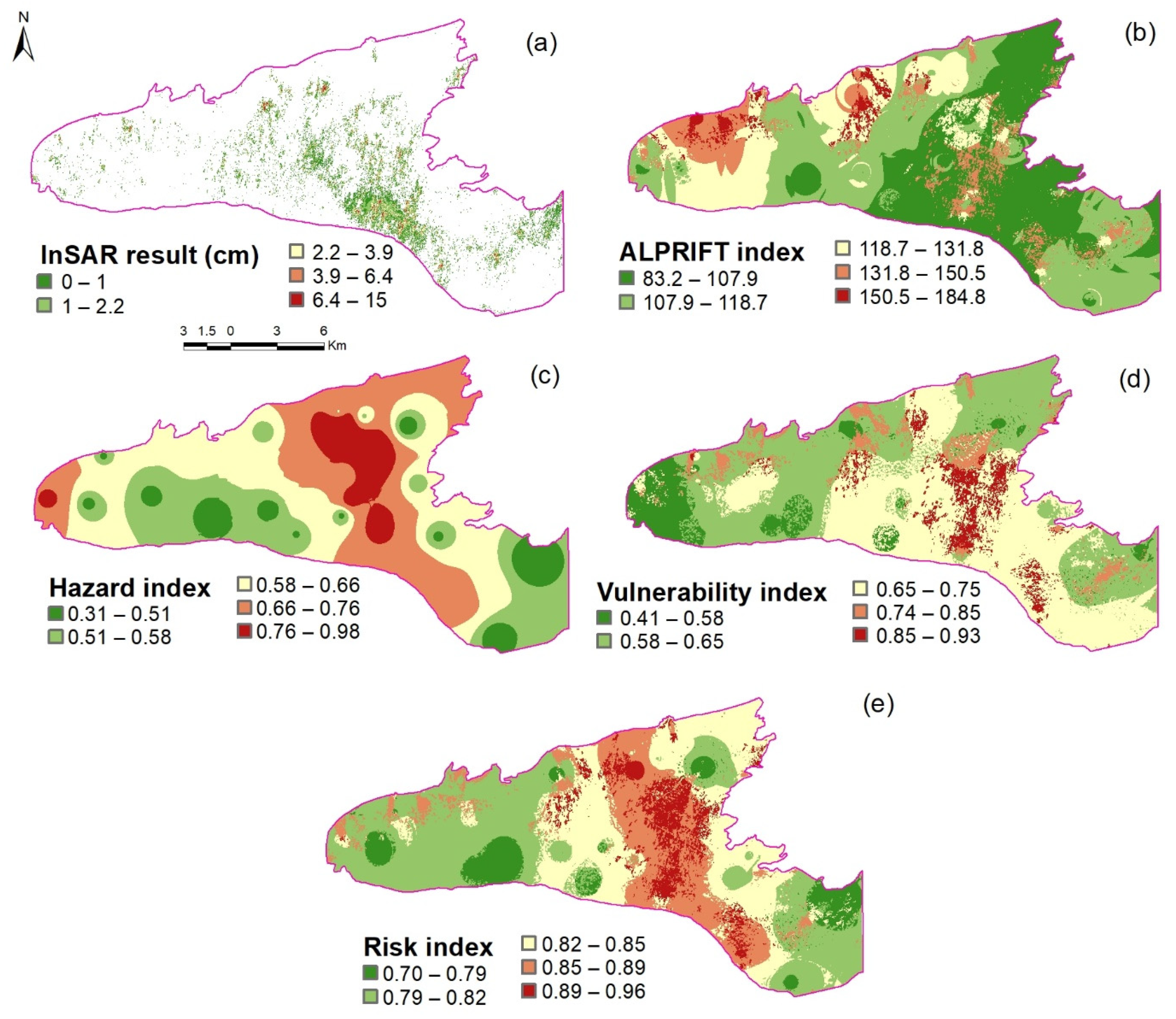
2.2. InSAR Processing

Based on the difference in the phase between two Sentinel-1 SAR observations, InSAR processes obtain information about the earth’s surface. InSAR processing leverages the amount of phase change between two consecutive and complete sine wave cycles. In particular, the phase follows the topography of the terrain. From the images and phase information in SAR systems, we can determine the strength of radar recognition from the amplitude information. The study used interferometric wide (IW) swath products with a spatial resolution of 5 m × 20 m and a swath of 250 km. A total of three sub-swaths are available here, based on terrain observation with progressive scans SAR (TOPSAR). A uniform signal-to-noise ratio (SNR) is provided along with a distributed target ambiguity ratio (DTAR) to produce homogeneous image quality throughout the swath. Several procedures are necessary to process InSAR data, including co-registration, interferogram formation, coherence estimation, phase removal from topography, phase filtering, phase unwrapping, terrain correction, and converting displacement along line-of-sight to vertical displacement. Further information about this procedure is available by [33].

2.3. Modeling Strategy at Level 1 by Fuzzy Catastrophe Scheme

FCS is used in the paper for mapping hazard, vulnerability, and risk at Level 1, where FCS reduces subjectivity in rates and weights of APLRIFT data layers. In MCDM, FCS is a technique developed by [34], bringing fuzzy membership analysis and catastrophe theory together. In fuzzy logic [35], membership functions, fuzzy sets, and fuzzy inference engines are used. According to [36], a catastrophe is the result of a set of dependent variables (also called state variables) and independent variables (also called control parameters). Recently, FCS was utilized in different fields of water resources, including ecological environment sustainability by [37], predicting harmful algae blooms by [38], aquifer vulnerability to LS by [6], and aquifer vulnerability to saltwater intrusion by [5].
As part of the catastrophe theory, a ranked list of functions can be assigned to the data layers, which include fold, cusp, swallowtail, butterfly, and wigwam. A state variable and control parameters ranging from 1 to 5 define these functions. Table 3 represents different types of catastrophe functions and related control parameters.
The formulated FCS includes: (i) hazard with two control parameters (PT data layers) then uses cusp, and (ii) vulnerability with five control parameters (ALRIF data layers) then uses wigwam. Therefore, FCS specifies the following functions for both hazard, vulnerability, and risk:
H a z a r d = 1 2 ( P 1 2 + T 1 3 )
V u l n e r a b i l i t y = 1 5 ( F 1 2 + I 1 3 + R 1 4 + L 1 5 + A 1 6 )
R i s k = H a z a r d × V u l n e r a b i l i t y
where Equations (4) and (5) contains two and five data layers, respectively. Data layers with higher weight gain the higher power, according to the recommendation of [12]. The mean operator calculates the system status based on the complementary principle; the alternative approach may be the minimum operator, which does not arise in the problem of LS. Notably, data layers in Equation (3) are normalized between 0 and 1 by linear membership functions as per the following equations:
X i n = X i X m i n X m a x X m i n
X i n = X m a x X i X m a x X m i n
where i counts pixels; Xmax and Xmin are maximum and minimum values, respectively; and X i n normalizes particular values at the ith pixels. Notably, Equation (7) normalizes data layers that are directly proportional to LS (A, L, P, I, T data layers); and Equation (8) normalizes data layers with inverse proportion (R, F data layers).

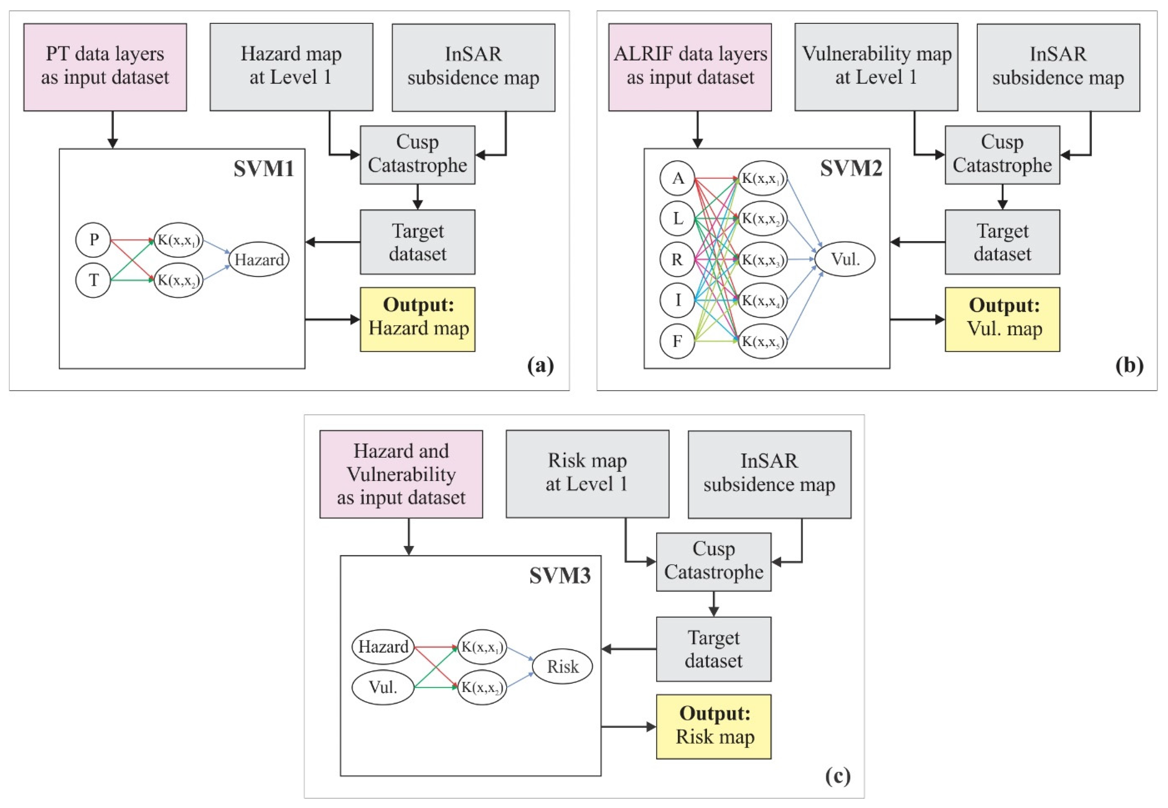
2.4. Modeling Strategy at Level 2 by SVM

SVM at Level 2 incorporates the Level 1 results in its structure. The input and target datasets of SVM is formulated as follows: (i) ALPRIFT data layers are input dataset; (ii) the data-fused of Level 1 result and InSAR subsidence map by catastrophe theory is considered as target datasets. Three SVMs are trained and tested for mapping supervised maps of hazard, vulnerability, and risk by SVM1, SVM2, and SVM3, respectively. Figure 1 summarizes the details in the architecture of SVMs. The target datasets for SVM1–SVM3 are calculated through Equations (9)–(11) based on the cusp catastrophe equation (see Table 3) as follows:
Target SVM 1 = [ H a z a r d   a t   L e v e l   1 ] 1 2 + [ I n S A R ] 1 3 2
Target SVM 2 = [ V u l .   a t   L e v e l   1 ] 1 2 + [ I n S A R ] 1 3 2
Target SVM 3 = [ R i s k   a t   L e v e l   1 ] 1 2 + [ I n S A R ] 1 3 2

2.5. Performance Metrics
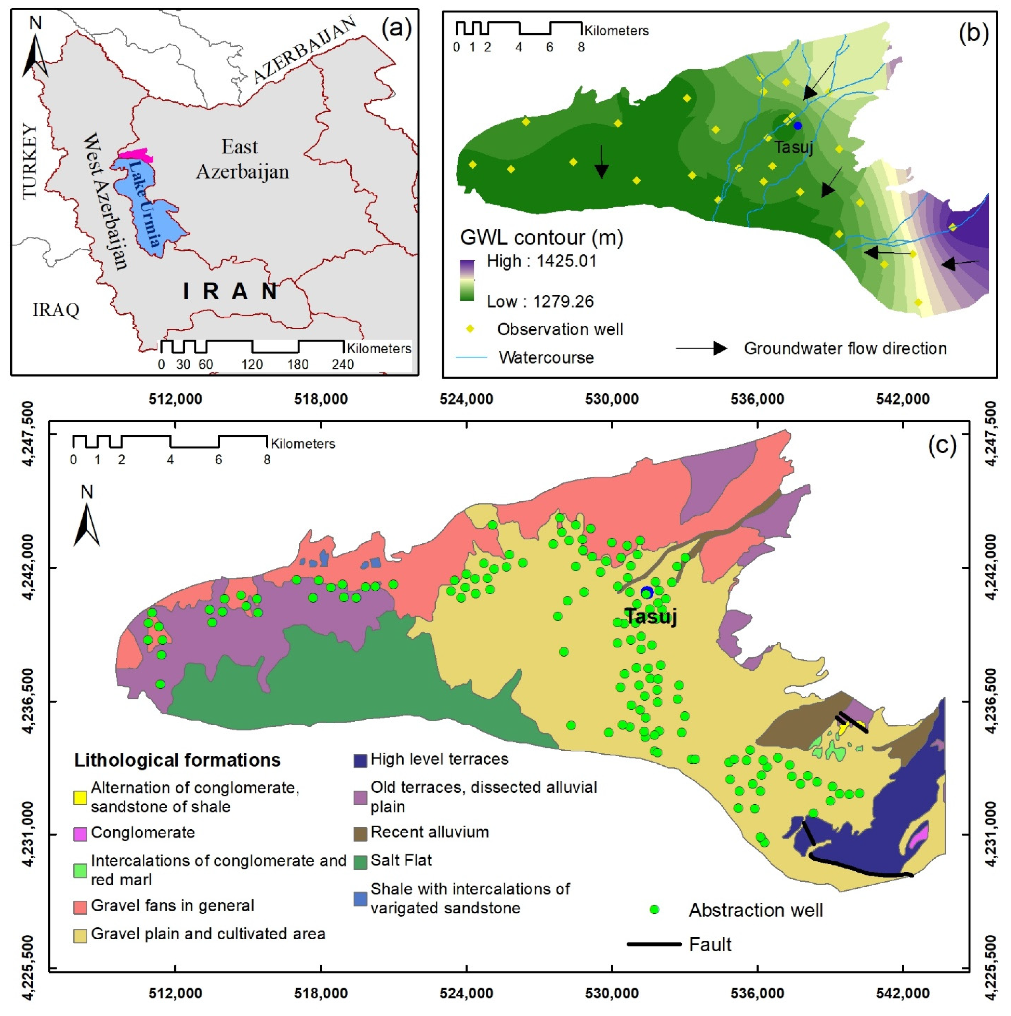
The performance of hazard, vulnerability, and risk indices concerning the InSAR result is evaluated by the receiver operating characteristic (ROC) curve and the area under curve (AUC). These criteria were developed by [31] to evaluate the precision of a diagnostic system, where the diagnosis refers to Earth’s displacement in the LS problem. The events related to diagnosis are divided into four groups of true negative (TN), true positive (TP), false positive (FP), and false negative (FN). Concerning the threshold of various settings, the ROC curve plots FP proportion against the TP proportion. An upper left corner deviation of the ROC curve corresponds to an undesirable performance. AUC measures the ratio of the area under the ROC curve compared to the total area ranging from 0.5 to 1. The AUC values equal to 1 and 0.5 correspond to the perfect and random performance, respectively.
The determination coefficient (R2) and root mean square error (RMSE) metrics evaluate the performance of SVM models. A value of R2 close to 1 represents the perfect performance, and a value close to zero shows unsatisfactory performance. Additionally, RMSE values close to 0 represent the best models, and it has no upper limit for unsatisfactory performance.

3. Study Area

This study is being conducted in the Tasuj plain, which lies with the province of East Azerbaijan in northwest Iran (see Figure 2). Additionally, this plain lies on the northern shores of Lake Urmia, where water levels have declined by about 15 m since 2000. At Tasuj climatological station, the average annual precipitation is 290 mm from 2008–2018, characterized by [39] as an arid and cold climate. The maximum and minimum temperatures are 33 °C and −11 °C during the same period. The area of the plain is about 300 km2 and generally is composed of alluvial sediments. In addition to the sedimentary deposit, igneous and metamorphosed formations are observable from Precambrian to the recent era. Figure 2 illustrates the lithological formations and the spatial location of the fault lines.
The sedimentary deposits form an unconfined aquifer as the primary source of water supply for agricultural and domestic purposes in the plain. The groundwater and surface water flow direction is towards Lake Urmia (see the flow direction in Figure 2b). The surface water is seasonal and is not a reliable source of water supply. The groundwater is discharged by 144 tube wells, 40 springs, and 70 qanats, which is equivalent to 16 × 106 m3 volume of water annually [40]. The groundwater level (GWL) in the aquifer is monitored monthly by 28 observation wells. The locations of the observation wells and abstraction wells are given in Figure 2b,c. The evaluation of the GWL time series in these wells shows that the GWL declined is 8.6 cm per month, which can trigger environmental problems such as LS. The paper presents the spatial distribution of subsidence captured by InSAR from 2017 to 2018 in due course.

4. Result

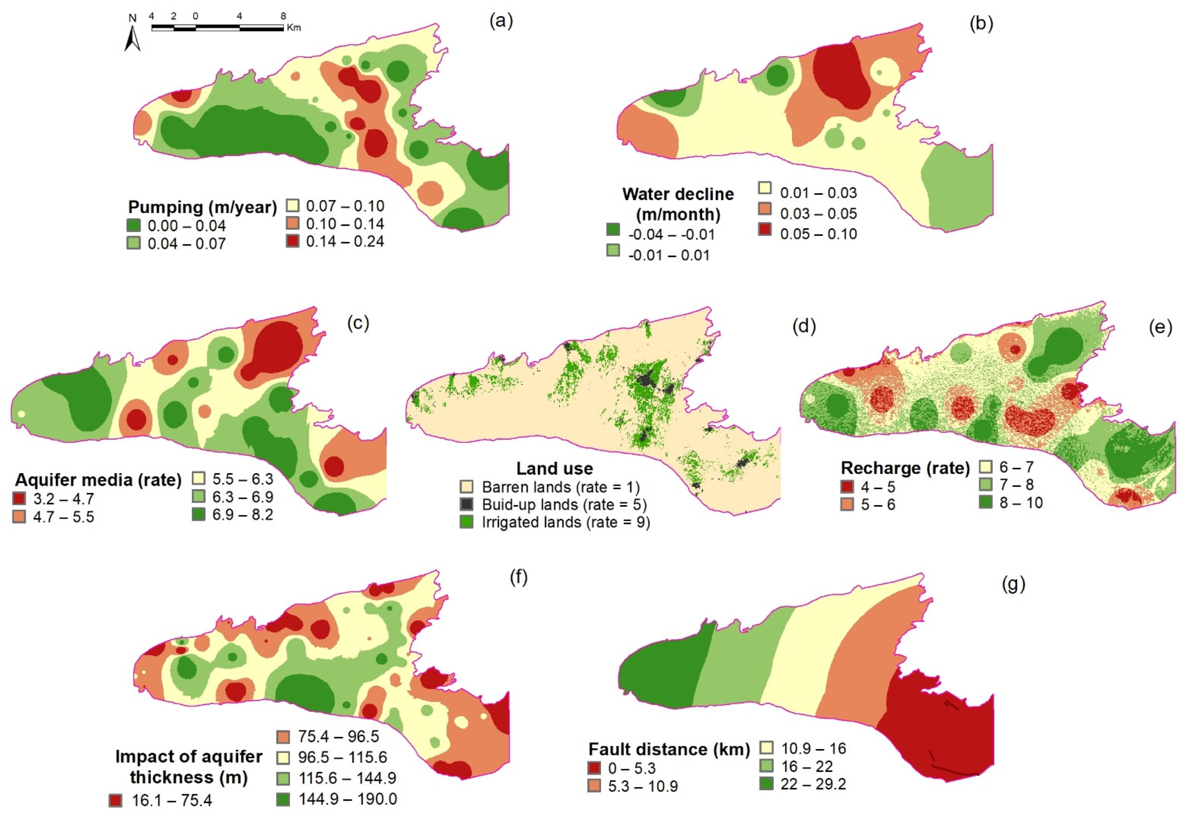
4.1. Preparation of ALPRIFT Data Layer

The data layers related to hazard (PT) and vulnerability (ALRIF) are prepared after pre-processing and GIS-processing as per Table 2. Figure 3 illustrates the spatial distribution of these data layers. A plot of the P- and T-data layers are depicted in Figure 3a,b based on pumping volume in abstraction wells and decline trend in observation wells, interpolated by the inverse distance weighting (IDW) technique.
In Figure 3c, aquifer media are calculated in geological logs as per aquifer media rates recommended by [12] and interpolated by IDW. The land use data layer is prepared by image processing through ENVI software. The required procedures are correcting the geometric and atmospheric, identifying different land using normalized difference vegetation index (NDVI), and interpreting images by the supervised classification approach to classify different land uses based on the maximum likelihood method. Figure 3d represents the land use data layer within the study area. The recharge data layer is calculated as per [41] using precipitation, infiltration, and slope data, and the result is presented in Figure 3e. The thickness of the aquifer in Figure 3f is calculated by geological logs and interpolated by IDW. In Figure 3g, a fault distance is calculated using the Euclidian distance toolbox available in the ArcGIS software.

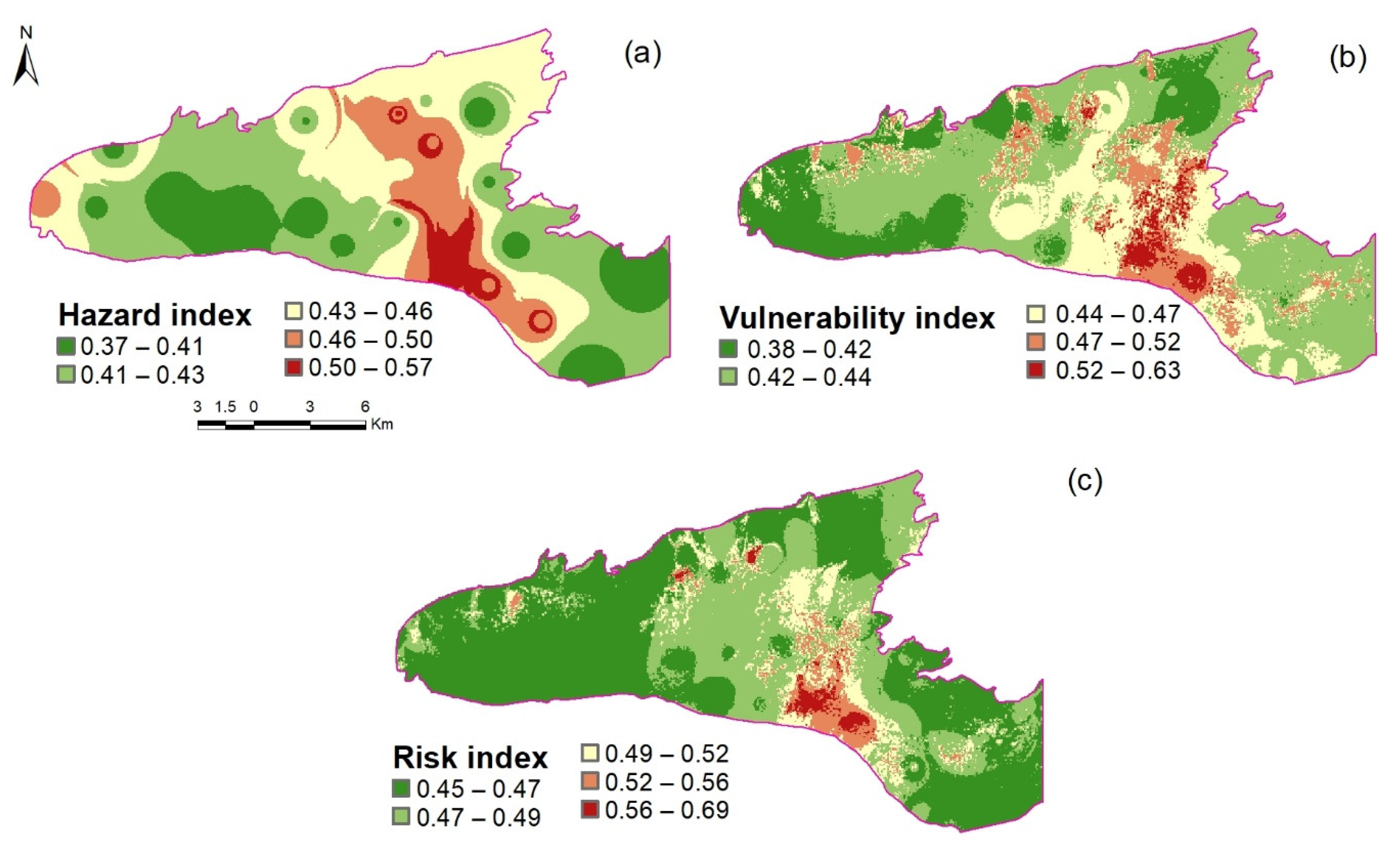
4.2. Results of InSARProcessing, Hazard, Vulnerability and Risk Indices at Level 1

Figure 4a illustrates the result of LS by InSAR processing from 2017 to 2018. The figure indicates that LS is mainly concentrated in the south-central part of the study area despite the scattered LS records elsewhere. The result of basic ALPRIFT is given in Figure 4b as per Equation (1) and the prescribed rates and weights by [12]. The comparison between Figure 4a,b indicates that the result of basic ALPRIFT is not entirely defensible, and there is room for improvement. Figure 4c,d represent, respectively, the hazard and vulnerability indices as per Equations (4) and (5). There are some similarities and differences between the spatial pattern of hazard and vulnerability indices, which is expected and stems from the incorporated data layers. The risk index pools together these similarities and differences as per Equation (6). Notably, hazard triggers a risk in areas with higher vulnerability, and this issue is illustrated in Figure 4e. A visual comparison between the InSAR result (Figure 4a) and the risk index (Figure 4e) indicates higher agreement than basic ALPRIFT, but there is still room for improvement.

4.3. Hazard, Vulnerability, and Risk Indices at Level 2

The hazard, vulnerability, and risk indices are calculated as per supervised learning by SVM1, SVM2, and SVM3, described in detail in Figure 1. Table 4 presents the performance criteria and SVM parameters for the hazard, vulnerability, and risk indices. The table evaluates the results regarding R2 and RMSE metrics for training, testing, and total datasets. According to the table, the models have similar performance in terms of both metrics in the training and testing phases. The spatial distribution of the results is given in Figure 5. Although there are similarities between this figure and the corresponding results in Figure 4, the results at Level 2 provide evidence that the Level 2 results are more compatible with the result of InSAR. The results at Level 2 identify the southcentral part of the study area as the hotspot area in terms of hazard, vulnerability, and risk.
The risk map in Figure 5c represents the hotspots with higher priorities for modifying management policies. However, this figure provides a relatively conservative result compared to the results of the hazard and vulnerability because the areas swept by Band 1 show a marked increase in risk potential. Additionally, some information in the hazard and vulnerability indices is not reflected in the risk index. For example, there are areas with a higher hazard index but a relatively lower vulnerability index in the north part of the plain. Thus, although human activities threaten these areas, they tend to be relatively less vulnerable, leading to a lower risk index.

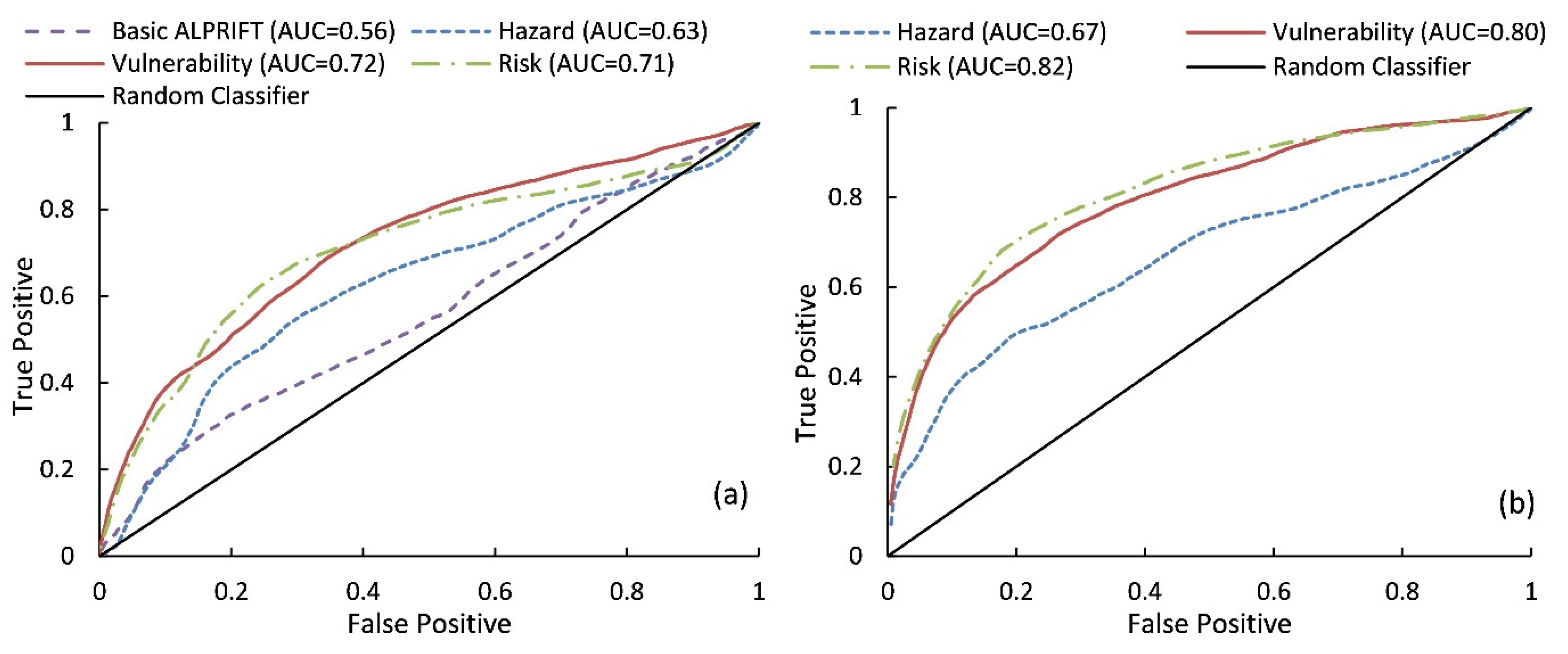
4.4. Evaluation of Results in Terms of ROC and AUC

Figure 6 evaluates the indices of basic ALPRIFT, hazard, vulnerability, and risk at Level 1 (Figure 6a) and Level 2 (Figure 6b) by the ROC curve and the AUC value. The figure indicates that the basic ALPRIFT provides noisy signals with the closest distance to the random classifier (the diagonal line). The AUC value for basic ALPRIFT is 0.56, which denotes that there is room for improvement. The ROC curve for hazard indices at Level 1 is slightly away from the random classifier line with an AUC value of 0.63. A similar improvement also is observed for the vulnerability and risk indices at Level 1, respectively, with AUC values of 0.72 and 0.71. This improvement refers to decreasing the subjectivities with rates and weights by FCS.
The results at Level 2 provide considerable improvements compared with the results at Level 1 as follows: (i) the AUC values for the hazard increases from 0.63 to 0.67; (ii) the AUC values for the vulnerability increases from 0.72 to 0.80; and (iii) the AUC values for the risk increases from 0.71 to 0.82. This improvement is expected due to using a learning technique by SVM. The lower AUC values for the hazard indices compared to vulnerability at both levels implies that the LS occurrence is more affected by intrinsic vulnerability than a man–made hazard. However, the hazard has a triggering role to risk since the ROC curve for the risk is somewhat higher than the vulnerability, and the AUC value for the risk index is slightly higher than the vulnerability index.

5. Discussion

ALPRIFT and similar frameworks are data–driven, and their results rely on data and the characteristics of study areas. These frameworks are in their infancy, and further investigations, such as using different modeling strategies, are required for proofing the concept. As discussed in Section 1, both MCDM and AI techniques were implemented on ALPRIFT in the previous studies. However, the paper combined two common approaches, and, in fact, it extended the MCDM–based study by [6] through considering a new level, which incorporates the Level 1 result as the target dataset in the formulation of Level 2.
The paper utilized a two–level multiple modeling strategy, referred to as inclusive multiple modeling (IMM), and the previous studies (e.g., [11]) indicated that IMM could significantly improve the modeling performance. As discussed earlier, the paper selected FCS at Level 1 and SVM at Level 2. There is no theoretical basis for model selection at both levels, and, generally, they are selected by a trial–and–error procedure. The idea for employing an MCDM technique at Level 1 and an AI technique at Level 2 stems from different formulations in the literature, which uses only AI approaches at both levels. However, FCS and SVM can be substituted with other techniques of MCDM and AI in future studies.
There is a significant difference between the AUC values related to the hazard and vulnerability maps. The paper identified that LS occurrence is more affected by intrinsic vulnerability than man–made hazard as per ROC/AUC. However, it should be noted that the man–made hazard triggers the LS, and it does not occur in the absence of over–abstraction, even with system vulnerabilities. Sadeghfam et al. [6] identified the man–made data layers as more effective than intrinsic data layers. This is expected because this issue is attributable to the characteristics of study areas. However, quantifying the role of these components provides more insight into risk management. Further investigation by statistical techniques is highly recommended to be undertaken to precisely identify the impact percentage of all components by future studies.
The investigation revealed that the hotspots identified by FCS at Level 1 occupy more areas compared to the hotspots by SVM. This is traceable to two issues: (i) The extent of areas with LS records is limited in the study area; and (ii) AI techniques are more powerful techniques in making a relationship between the input data layers and LS captured by InSAR even though the target dataset is fused by the Level 1 results. There seems to be room for investigating the role of others data fusion techniques in preparing target datasets in future studies.

6. Conclusions

ALPRIFT as a standard framework quantifies aquifers’ vulnerability to land subsidence (LS), but it suffers subjectivity associated with the incorporated data layers. The paper formulated a methodology based on inclusive multiple modeling (IMM) at two levels to decrease the subjectivity and increase the modeling performance. IMM also map the hazard, vulnerability, and risk indices to LS, in which a fuzzy catastrophe scheme as a multi–criteria decision making (MCDM) technique was used at Level 1; and the obtained results were feed as the target dataset to the support vector machine as an artificial intelligence (AI) technique at Level 2. Therefore, the formulated methodology combines two capabilities of MCDM and AI. The formulation was implemented in Tasuj plain, located in northwest Iran, which suffers from over–abstraction. Results at both levels identify significant signals as per the receiver operating characteristic and the area under curve (AUC) performance metrics for the hazard, vulnerability, and risk indices. Additionally, further improvements were achieved from Levels 1 to 2 for the vulnerability and risk indices, which is expected due to the capability of IMM. However, there is room for further improvements in the performance of results by future studies. The higher AUC values for the vulnerability index on recorded LS compared to the hazard index indicated that the LS occurrence in the study area is more affected by the intrinsic vulnerability of the system, but anthropogenic activities play an actuation role in the risk realization.

Author Contributions

A.A.N. and S.S. designed modeling concepts and wrote the manuscript and check the results. M.M. prepared the framework and implemented the models. R.B. did preprocesses and prepared datasets and grammatically checked the text. All authors have read and agreed to the published version of the manuscript.

Funding

The project was supported financially by the University of Tabriz (Grant ID: 4349).

Institutional Review Board Statement

Not applicable.

Informed Consent Statement

Not applicable.

Data Availability Statement

Not applicable.

Conflicts of Interest

The authors declare no conflict of interest.

References

  1. Jhariya, D.C.; Kumar, T.; Pandey, H.K.; Kumar, S.; Kumar, D.; Gautam, A.K.; Kishore, N. Assessment of groundwater vulnerability to pollution by modified DRASTIC model and analytic hierarchy process. Environ. Earth Sci. 2019, 78, 1–20. [Google Scholar] [CrossRef]
  2. Garewal, S.K.; Vasudeo, A.D.; Landge, V.S.; Ghare, A.D. A GIS-based Modified DRASTIC (ANP) method for assessment of groundwater vulnerability: A case study of Nagpur city, India. Water Qual. Res. 2015, 52, 121–135. [Google Scholar] [CrossRef]
  3. Andualem, T.G.; Demeke, G.G. Groundwater potential assessment using GIS and remote sensing: A case study of Guna tana landscape, upper blue Nile Basin, Ethiopia. J. Hydrol. Reg. Stud. 2019, 24, 100610. [Google Scholar] [CrossRef]
  4. Sadeghfam, S.; Hassanzadeh, Y.; Nadiri, A.A.; Zarghami, M. Localization of groundwater vulnerability assessment using catastrophe theory. Water Resour. Manag. 2016, 30, 4585–4601. [Google Scholar] [CrossRef]
  5. Sadeghfam, S.; Khatibi, R.; Daneshfaraz, R.; Rashidi, H.B. Transforming vulnerability indexing for saltwater intrusion into risk indexing through a fuzzy catastrophe scheme. Water Resour. Manag. 2020, 34, 175–194. [Google Scholar] [CrossRef]
  6. Sadeghfam, S.; Khatibi, R.; Dadashi, S.; Nadiri, A.A. Transforming subsidence vulnerability indexing based on ALPRIFT into risk indexing using a new fuzzy-catastrophe scheme. Environ. Impact Assess. Rev. 2020, 82, 106352. [Google Scholar] [CrossRef]
  7. Band, S.S.; Janizadeh, S.; Pal, S.C.; Chowdhuri, I.; Siabi, Z.; Norouzi, A.; Mosavi, A. Comparative analysis of artificial intelligence models for accurate estimation of groundwater nitrate concentration. Sensors 2020, 20, 5763. [Google Scholar] [CrossRef] [PubMed]
  8. Nguyen, P.T.; Ha, D.H.; Jaafari, A.; Nguyen, H.D.; Van Phong, T.; Al-Ansari, N.; Pham, B.T. Groundwater potential mapping combining artificial neural network and real AdaBoost ensemble technique: The DakNong province case-study, Vietnam. Int. J. Environ. Res. Public Health 2020, 17, 2473. [Google Scholar] [CrossRef] [Green Version]
  9. Moazamnia, M.; Hassanzadeh, Y.; Nadiri, A.A.; Sadeghfam, S. Vulnerability indexing to saltwater intrusion from models at two levels using artificial intelligence multiple model (AIMM). J. Environ. Manag. 2020, 255, 109871. [Google Scholar] [CrossRef] [PubMed]
  10. Sadeghfam, S.; Nourbakhsh Khiyabani, F.; Khatibi, R.; Daneshfaraz, R. A study of land subsidence problems by ALPRIFT for vulnerability indexing and risk indexing and treating subjectivity by strategy at two levels. J. Hydroinform. 2020, 22, 1640–1662. [Google Scholar] [CrossRef]
  11. Gharekhani, M.; Nadiri, A.A.; Khatibi, R.; Sadeghfam, S. An investigation into time-variant subsidence potentials using inclusive multiple modelling strategies. J. Environ. Manag. 2021, 294, 112949. [Google Scholar] [CrossRef] [PubMed]
  12. Nadiri, A.A.; Taheri, Z.; Khatibi, R.; Barzegari, G.; Dideban, K. Introducing a new framework for mapping subsidence vulnerability indices (SVIs): ALPRIFT. Sci. Total Environ. 2018, 628, 1043–1057. [Google Scholar] [CrossRef] [PubMed]
  13. Arabameri, A.; Pal, S.C.; Rezaie, F.; Chakrabortty, R.; Chowdhuri, I.; Blaschke, T.; Ngo, P.T.T. Comparison of multi-criteria and artificial intelligence models for land-subsidence susceptibility zonation. J. Environ. Manag. 2021, 284, 112067. [Google Scholar] [CrossRef] [PubMed]
  14. Ebrahimy, H.; Feizizadeh, B.; Salmani, S.; Azadi, H. A comparative study of land subsidence susceptibility mapping of Tasuj plane, Iran, using boosted regression tree, random forest and classification and regression tree methods. Environ. Earth Sci. 2020, 79, 1–12. [Google Scholar] [CrossRef]
  15. Nadiri, A.A.; Khatibi, R.; Khalifi, P.; Feizizadeh, B. A study of subsidence hotspots by mapping vulnerability indices through innovatory ‘ALPRIFT’ using artificial intelligence at two levels. Bull. Eng. Geol. Environ. 2020, 79, 3989–4003. [Google Scholar] [CrossRef]
  16. Mohammady, M.; Pourghasemi, H.R.; Amiri, M. Assessment of land subsidence susceptibility in Semnan plain (Iran): A comparison of support vector machine and weights of evidence data mining algorithms. Nat. Hazards 2019, 99, 951–971. [Google Scholar] [CrossRef]
  17. Perrin, J.; Cartannaz, C.; Noury, G.; Vanoudheusden, E. A multicriteria approach to karst subsidence hazard mapping supported by weights-of-evidence analysis. Eng. Geol. 2015, 197, 296–305. [Google Scholar] [CrossRef]
  18. Pradhan, B.; Abokharima, M.H.; Jebur, M.N.; Tehrany, M.S. Land subsidence susceptibility mapping at Kinta Valley (Malaysia) using the evidential belief function model in GIS. Nat. Hazards 2014, 73, 1019–1042. [Google Scholar] [CrossRef]
  19. Abdollahi, S.; Pourghasemi, H.R.; Ghanbarian, G.A.; Safaeian, R. Prioritization of effective factors in the occurrence of land subsidence and its susceptibility mapping using an SVM model and their different kernel functions. Bull. Eng. Geol. Environ. 2019, 78, 4017–4034. [Google Scholar] [CrossRef]
  20. Rehman, S.; Sahana, M.; Dutta, S.; Sajjad, H.; Song, X.; Imdad, K.; Dou, J. Assessing subsidence susceptibility to coal mining using frequency ratio, statistical index and Mamdani fuzzy models: Evidence from Raniganj coalfield, India. Environ. Earth Sci. 2020, 79, 1–18. [Google Scholar] [CrossRef]
  21. Najafi, Z.; Pourghasemi, H.R.; Ghanbarian, G.; Shamsi, S.R.F. Land-subsidence susceptibility zonation using remote sensing, GIS, and probability models in a Google Earth Engine platform. Environ. Earth Sci. 2020, 79, 1–16. [Google Scholar] [CrossRef]
  22. Arabameri, A.; Saha, S.; Roy, J.; Tiefenbacher, J.P.; Cerda, A.; Biggs, T.; Collins, A.L. A novel ensemble computational intelligence approach for the spatial prediction of land subsidence susceptibility. Sci. Total Environ. 2020, 726, 138595. [Google Scholar] [CrossRef] [PubMed]
  23. Guoqing, Y.; Jingqin, M. D-InSAR technique for land subsidence monitoring. Earth Sci. Front. 2008, 15, 239–243. [Google Scholar] [CrossRef]
  24. Ge, L.; Ng, A.H.M.; Li, X.; Abidin, H.Z.; Gumilar, I. Land subsidence characteristics of Bandung Basin as revealed by ENVISAT ASAR and ALOS PALSAR interferometry. Remote Sens. Environ. 2014, 154, 46–60. [Google Scholar] [CrossRef]
  25. Chaussard, E.; Wdowinski, S.; Cabral-Cano, E.; Amelung, F. Land subsidence in central Mexico detected by ALOS InSAR time-series. Remote Sens. Environ. 2014, 140, 94–106. [Google Scholar] [CrossRef]
  26. Pacheco-Martínez, J.; Wdowinski, S.; Cabral-Cano, E.; Hernández-Marín, M.; Ortiz-Lozano, J.A.; Oliver-Cabrera, T.; Havazli, E. Application of InSAR and gravimetric surveys for developing construction codes in zones of land subsidence induced by groundwater extraction: Case study of Aguascalientes, Mexico. Proc. Int. Assoc. Hydrol. Sci. 2015, 372, 121–127. [Google Scholar] [CrossRef] [Green Version]
  27. Zuo, J.; Gong, H.; Chen, B.; Liu, K.; Zhou, C.; Ke, Y. Time-series evolution patterns of land subsidence in the eastern Beijing Plain, China. Remote Sens. 2019, 11, 539. [Google Scholar] [CrossRef] [Green Version]
  28. Jiang, H.; Balz, T.; Cigna, F.; Tapete, D. Land Subsidence in Wuhan Revealed Using a Non-Linear PSInSAR Approach with Long Time Series of COSMO-SkyMed SAR Data. Remote Sens. 2021, 13, 1256. [Google Scholar] [CrossRef]
  29. Chen, C.H.; Lin, Z.S. A committee machine with empirical formulas for permeability prediction. Comput. Geosci. 2006, 32, 485–496. [Google Scholar] [CrossRef]
  30. Kadkhodaie-Ilkhchi, A.; Rezaee, M.R.; Rahimpour-Bonab, H.; Chehrazi, A. Petrophysical data prediction from seismic attributes using committee fuzzy inference system. Comput. Geosci. 2009, 35, 2314–2330. [Google Scholar] [CrossRef] [Green Version]
  31. Swets, J.A. Measuring the accuracy of diagnostic systems. Science 1988, 240, 1285–1293. [Google Scholar] [CrossRef] [Green Version]
  32. UN Office for Disaster Risk ReductionLiving with Risk. A Global Review of Disaster Reduction Initiatives; United Nations Publications: Geneva, Switzerland, 2004; ISBN 9211010640. [Google Scholar]
  33. Hanssen, R.F. Radar Interferometry: Data Interpretation and Error Analysis; Kluwer Academic Publishers: Dordrecht, The Netherlands, 2001. [Google Scholar]
  34. Cheng, C.H.; Liu, Y.H.; Lin, Y. Evaluating a weapon system using catastrophe series based on fuzzy scales. In Soft Computing in Intelligent Systems and Information Processing, Proceedings of the 1996 Asian Fuzzy Systems Symposium, Kent-ing, Taiwan, 6 August 2002; IEEE: Piscataway, NJ, USA, 2002; pp. 212–217. [Google Scholar] [CrossRef]
  35. Zadeh, L.A. Fuzzy sets as a basis for a theory of possibility. Fuzzy Sets Syst. 1965, 338–353. [Google Scholar] [CrossRef]
  36. Thom, R. Stabilité structurelle et morphogénèse. Poetics 1974, 3, 7–19. [Google Scholar] [CrossRef]
  37. Gao, S.; Sun, H.; Zhao, L.; Wang, R.; Xu, M.; Cao, G. Dynamic assessment of island ecological environment sustainability under urbanization based on rough set, synthetic index and catastrophe progression analysis theories. Ocean Coast. Manag. 2019, 178, 104790. [Google Scholar] [CrossRef]
  38. Tian, Y.; Zheng, B.; Shen, H.; Zhang, S.; Wang, Y. A novel index based on the cusp catastrophe theory for predicting harmful algae blooms. Ecol. Indic. 2019, 102, 746–751. [Google Scholar] [CrossRef]
  39. Emberger, L. Climate on a formula applicable in botanical geography. Comptes Rendus L’académie Sci. 1930, 191, 389–390. [Google Scholar]
  40. East Azerbaijan Water Authority Provided the Data through Private Communications. Available online: http://www.azarwater.ir/?l=EN (accessed on 13 August 2021).
  41. Piscopo, G. Groundwater Vulnerability Map; Ex planatory Notes, Castlereagh Catchment, NSW; Department of Land and Water Conservation: Parramatta, Australia, 2001.
Figure 1. Methodological flowchart for mapping: (a) supervised hazard; (b) supervised vulnerability; and (c) supervised risk.
Water 13 02622 g001
Figure 2. Study area: (a) location map; (b) GWL and observation wells; (c) lithological map and abstraction wells.
Water 13 02622 g002
Figure 3. Hazard data layers: (a) pumping of groundwater; (b) water table decline; and vulnerability data layers: (c) aquifer media; (d) land use; (e) recharge; (f) impact of aquifer thickness; (g) fault distance.
Water 13 02622 g003
Figure 4. (a) InSAR result; (b) basic ALPRIFT; (c) hazard at Level 1; (d) vulnerability at Level 1; (e) risk at Level 1.
Water 13 02622 g004
Figure 5. Result at Level 2: (a) hazard; (b) vulnerability; (c) risk.
Water 13 02622 g005
Figure 6. Performance evaluation by ROC/AUC: (a) results at Level 1; (b) results at Level 2.
Water 13 02622 g006
Table 1. Summarized studies to calculate the land susceptibility index or LS hazard mapping.
ReferenceApproachIncorporated Data Layers
[18]StatisticalAltitude, Slope, Aspect, Lithology, Distance from the fault, Distance from the river, Normalized difference vegetation index, Soil type, Stream power index, Topographic wetness index, Land use/Land cover
[17]MCDMCover thickness, Low permeability layer thickness, Distance to losing streams, Saturated cover thickness
[19]AIPercentage slope, Slope aspect, Altitude, Profile curvature, Plan curvature, Topographic wetness index, Distance from river, Lithological, Units, Piezometric data, Land use, Normalized difference vegetation index
[16]AIElevation, Slope angle, Slope aspect, Topographic wetness index, Plan curvature, Profile curvature, Lithology, Land use, Drainage network, Roads, Faults, Groundwater table
[20]AIGeology, Lineament, Land use/Land cover, Rainfall distribution, Slope, Slope aspect, Coal seam proximity, Curvature, Distance from road, Drainage density, Drainage proximity, Elevation, Soil, Stream power index, Topographical wetness index
[21]StatisticalAltitude, Slope aspect, Land use, Distance from the faults, Lithology, Plan curvature, Distance from river, Slope percent, Piezometric data, Topographic wetness index
[22]AIGroundwater drawdown, Land use/Land cover, Elevation, Lithology, Drainage density, Distance to stream, Distance to road, Slope, Topographical Wetness index, Profile curvature, Aspect, Plan curvature
[14]AI and MCDMAltitude, Slope angle, Aspect, Groundwater level, Groundwater level change, Land cover, Lithology, Distance to fault, Distance to stream, Stream power index, Topographic wetness index, Plan curvature
[13]AI and MCDMLithology, Plan Curvature, Profile Curvature, Slope, Topographical Wetness Index, Aspect, Elevation, Drainage Density, Distance to road, Distance to stream, Groundwater, Land Use/land Cover
Table 2. Required input datasets and GIS-processing for ALPRIFT data layers.
Data LayerInput DatasetProcessing
HazardPumping of groundwater (P)Annual discharge at abstraction wellsDraw Thiessen polygon
Interpolate by Inverse Distance Weighted (IDW) technique
Water Table decline trend (T)GWL time seriesCalculate trend of decline
Interpolate by IDW
VulnerabilityAquifer media (A)Geological logsAssign ALPRIFT rates
Interpolate by IDW
Land use (L)Satellite image
(Sentinel-1)
Image Processing
Recharge (R)Slope
Soil permeability
Precipitation
Reclassify
Overlay [31]
Impact of aquifer thickness (I)Geoelectric profilesInterpolate by IDW
Fault distance (F)Fault mapEuclidean distance tool
Table 3. Catastrophe functions [6,34].
NameState VariableControl ParameterCatastrophe Fuzzy Membership Functions
Fold11 x a = a 2
Cusp12 x a = a 2 ,   x b = b 3
Swallowtail13 x a = a 2 ,   x b = b 3 ,   x c = c 4
Butterfly14 x a = a 2 ,   x b = b 3 ,   x c = c 4 , x d = d 5
Wigwam15 x a = a 2 ,   x b = b 3 ,   x c = c 4 , x d = d 5 , x e = e 6
Note that: a, b, c, d, e are control parameters. xa, xb, xc, xd, xe are state variables.
Table 4. Performance criteria for developed SVM at Level 2.
R2RMSE
TrainingTestingTotalTrainingTestingTotal
Hazard0.710.700.710.0260.0260.45
Vulnerability0.720.720.720.0290.0280.44
Risk0.740.740.740.0270.0270.48
The SVM parameters: γ = 15, σ = 0.2.
Publisher’s Note: MDPI stays neutral with regard to jurisdictional claims in published maps and institutional affiliations.

