
Geophysical Delineation of Freshwater–Saline Water Interfaces in Coastal Area of Southwest Bangladesh

 , ,
, ,  , , , and
Abstract
:1. Introduction
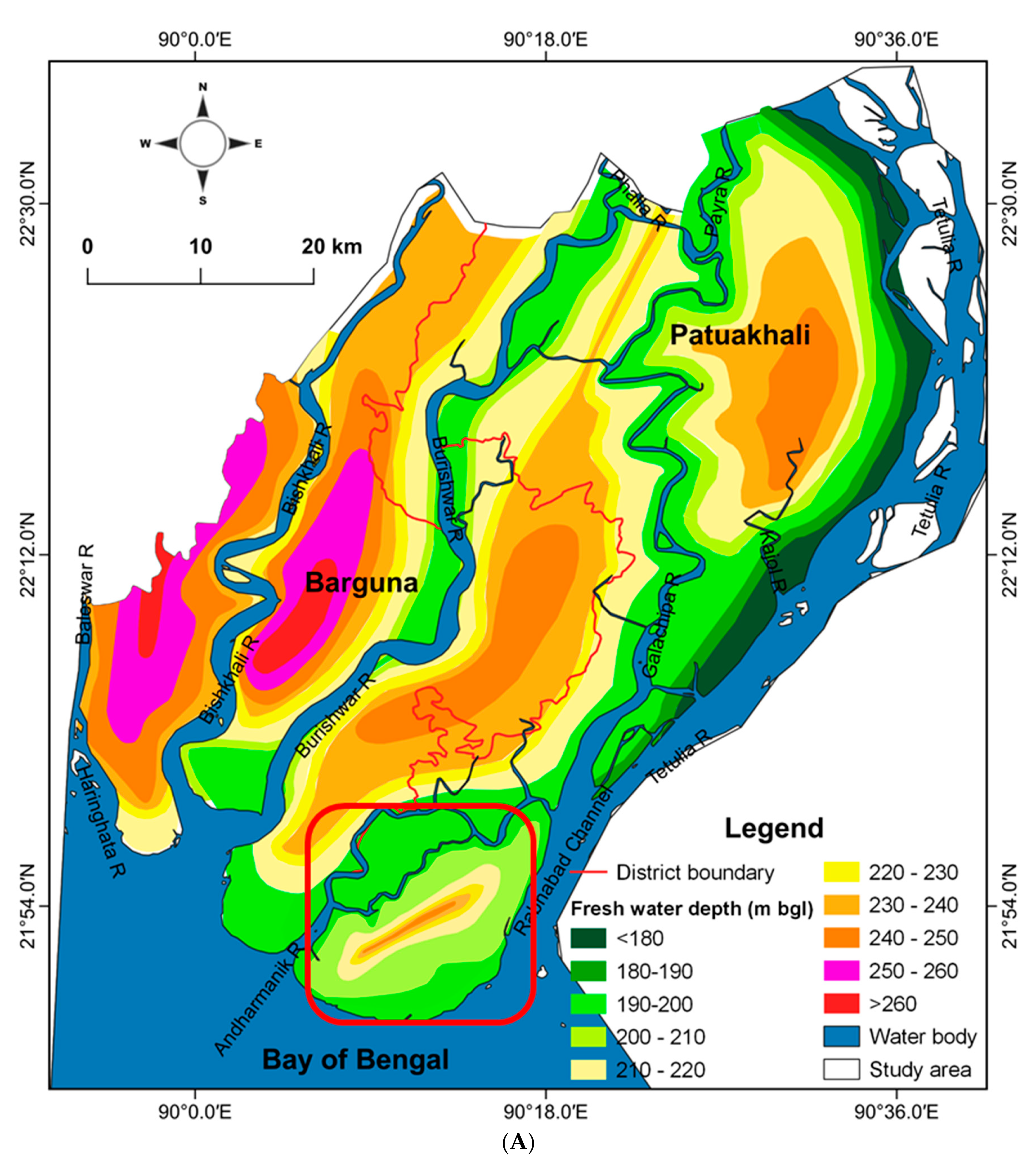
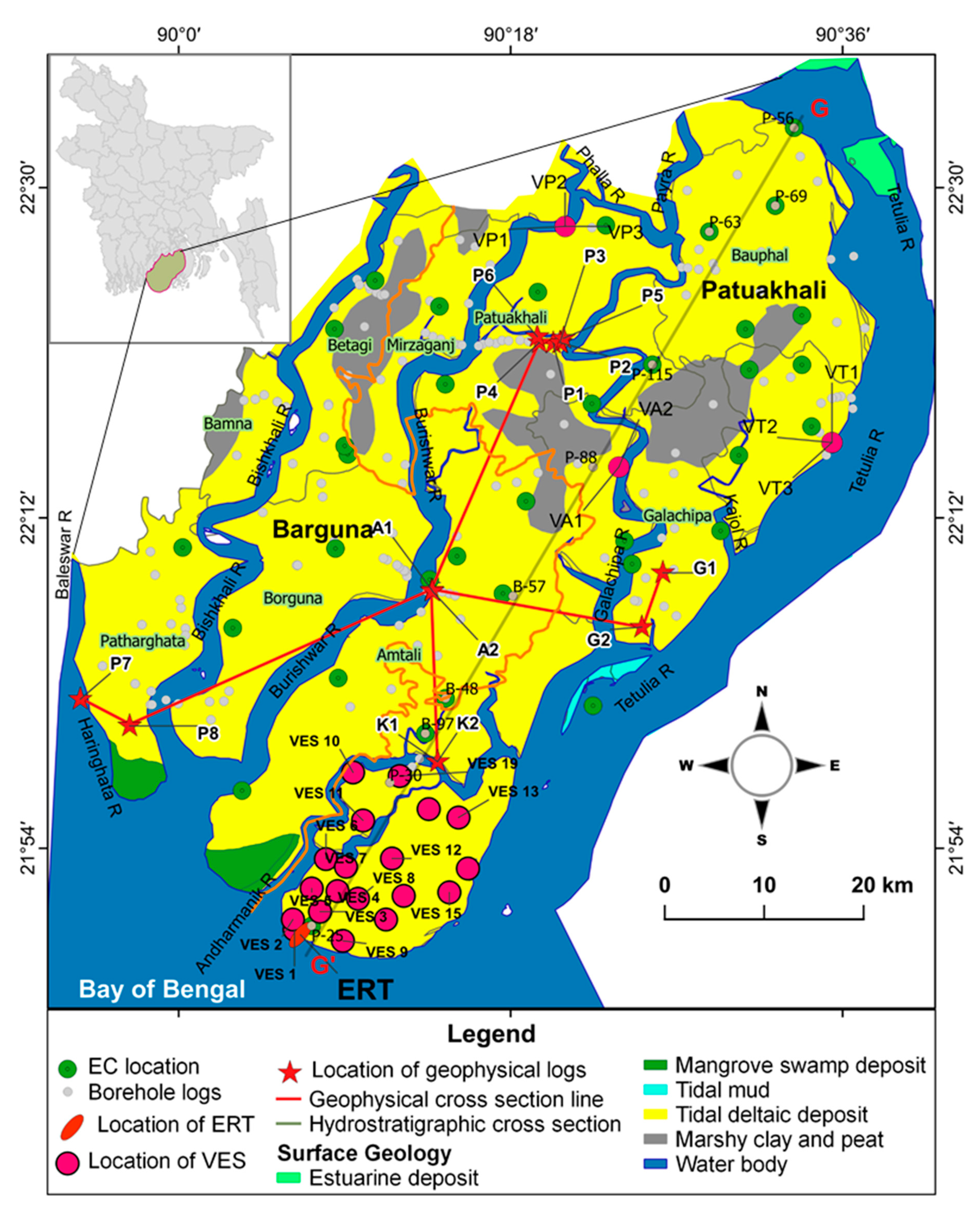
2. Study Area
2.1. Hydrology and Climate
2.2. Geology and Hydrogeology
3. Materials and Methods
3.1. Geophysical Prospection
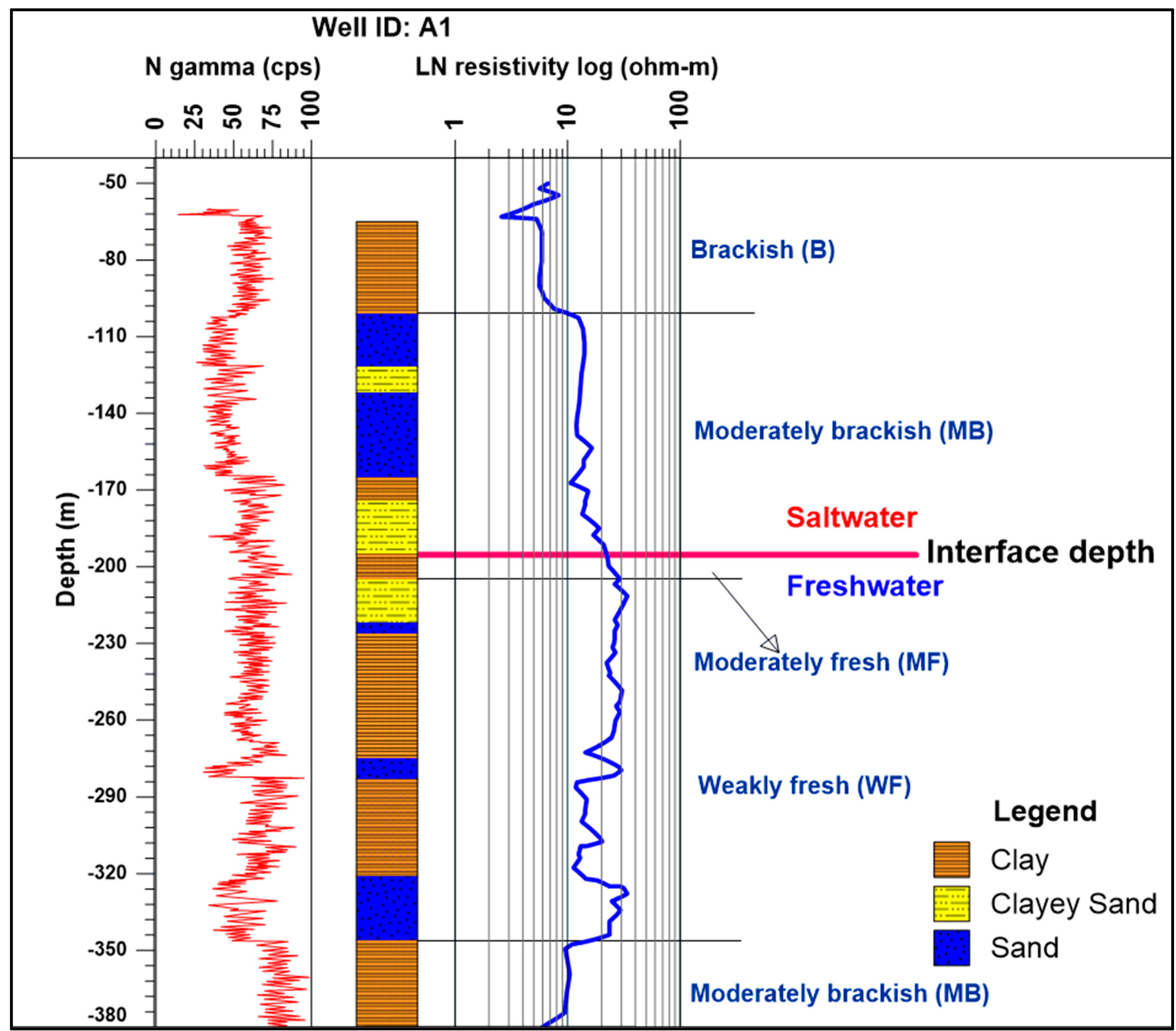
3.1.1. Geophysical Well Logs
3.1.2. Resistivity Ground Surveys
- 1-D inversion
- ERT
- Depth of Investigation (DOI) Index
3.2. Determination of Pore-Water Resistivity
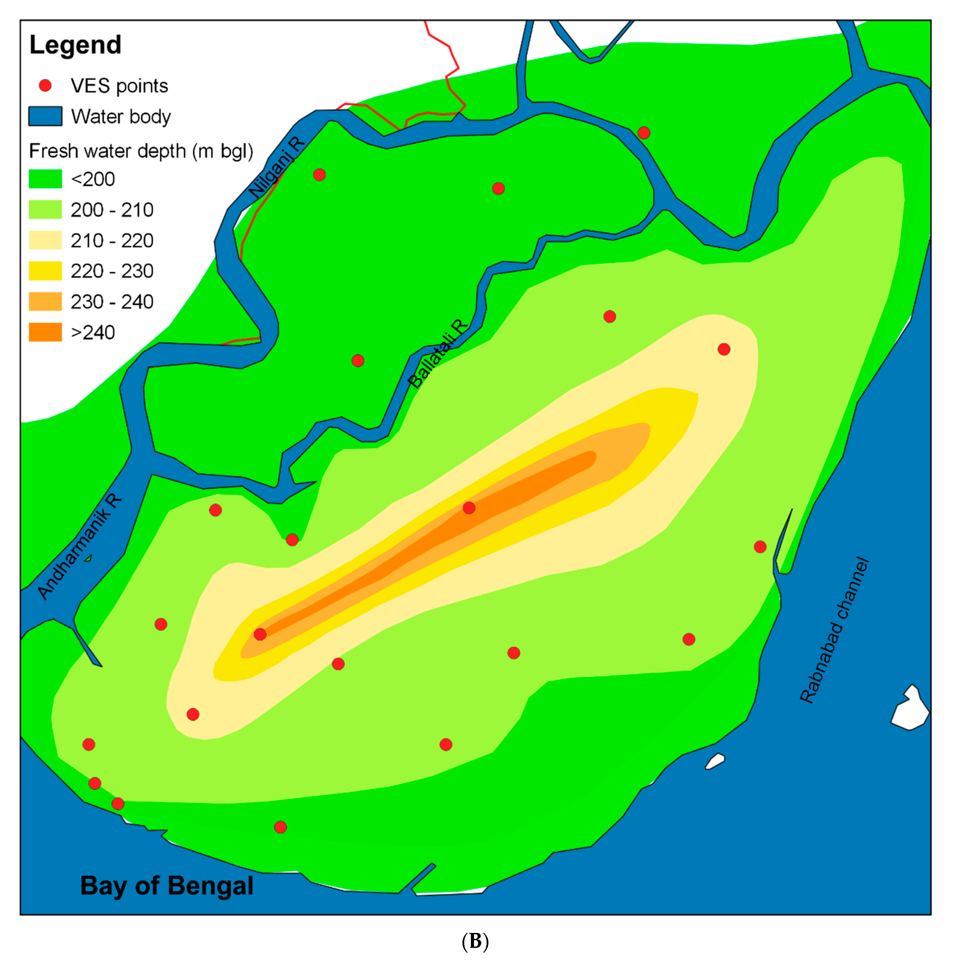
3.3. Saltwater–Freshwater Interface Map
4. Results
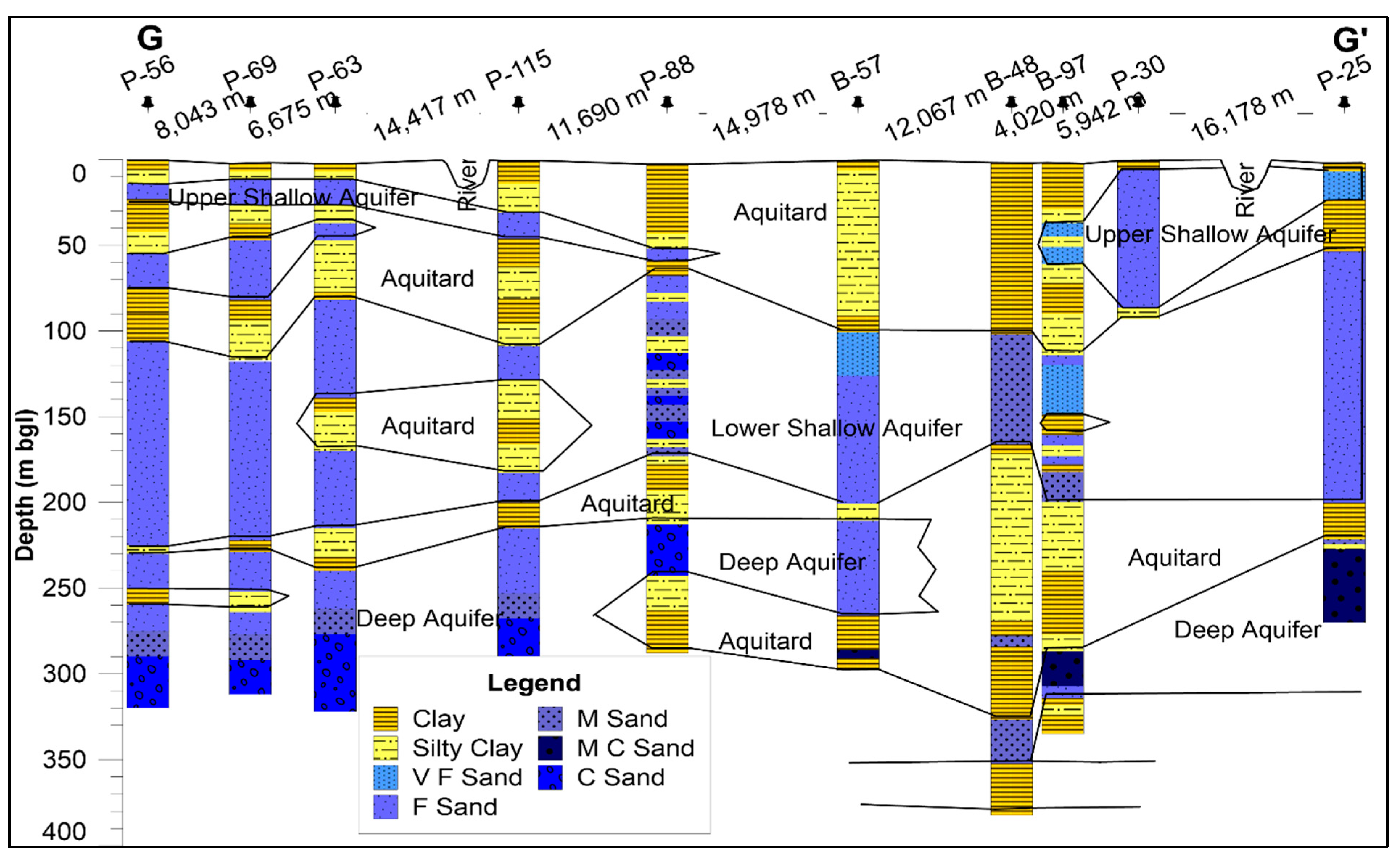
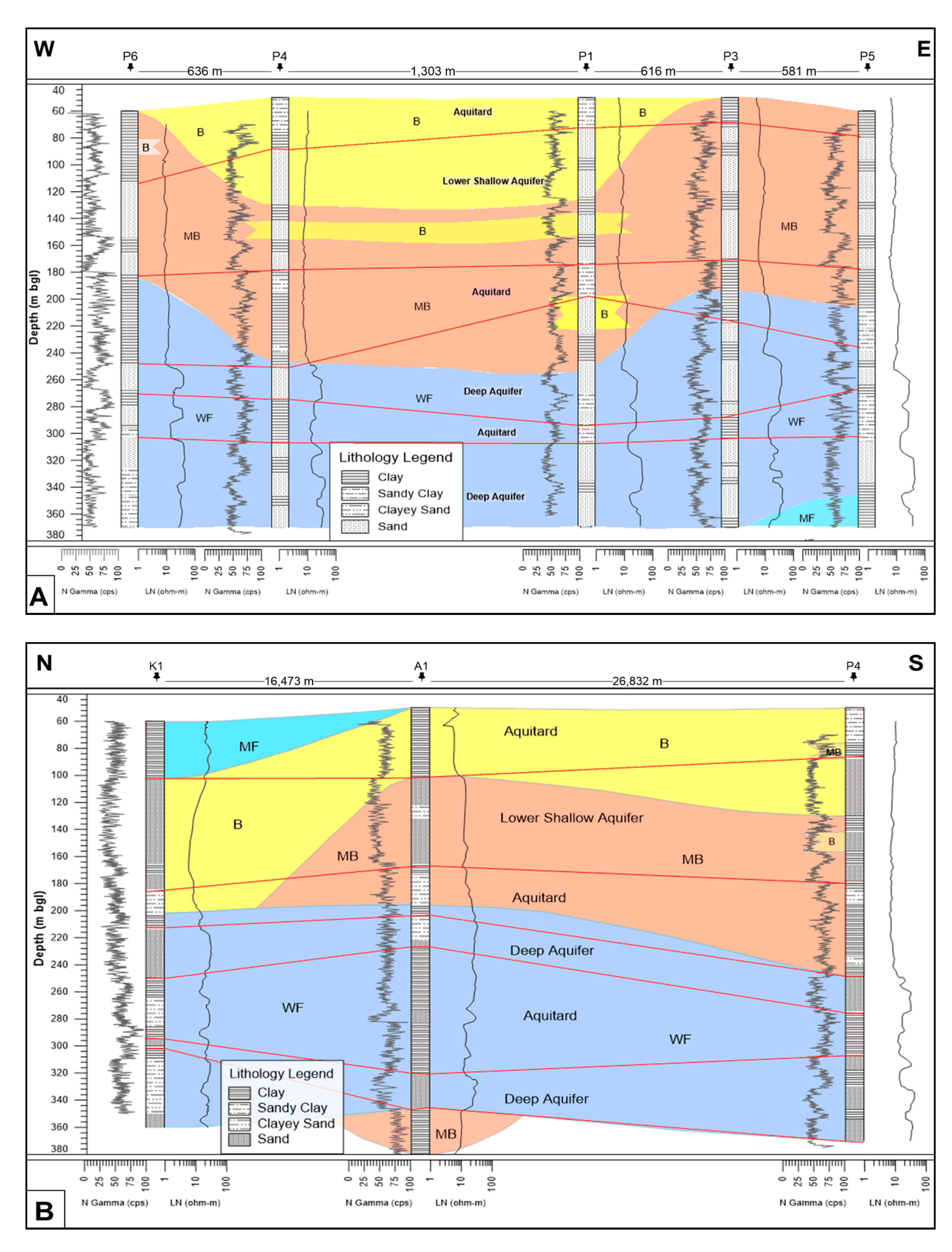
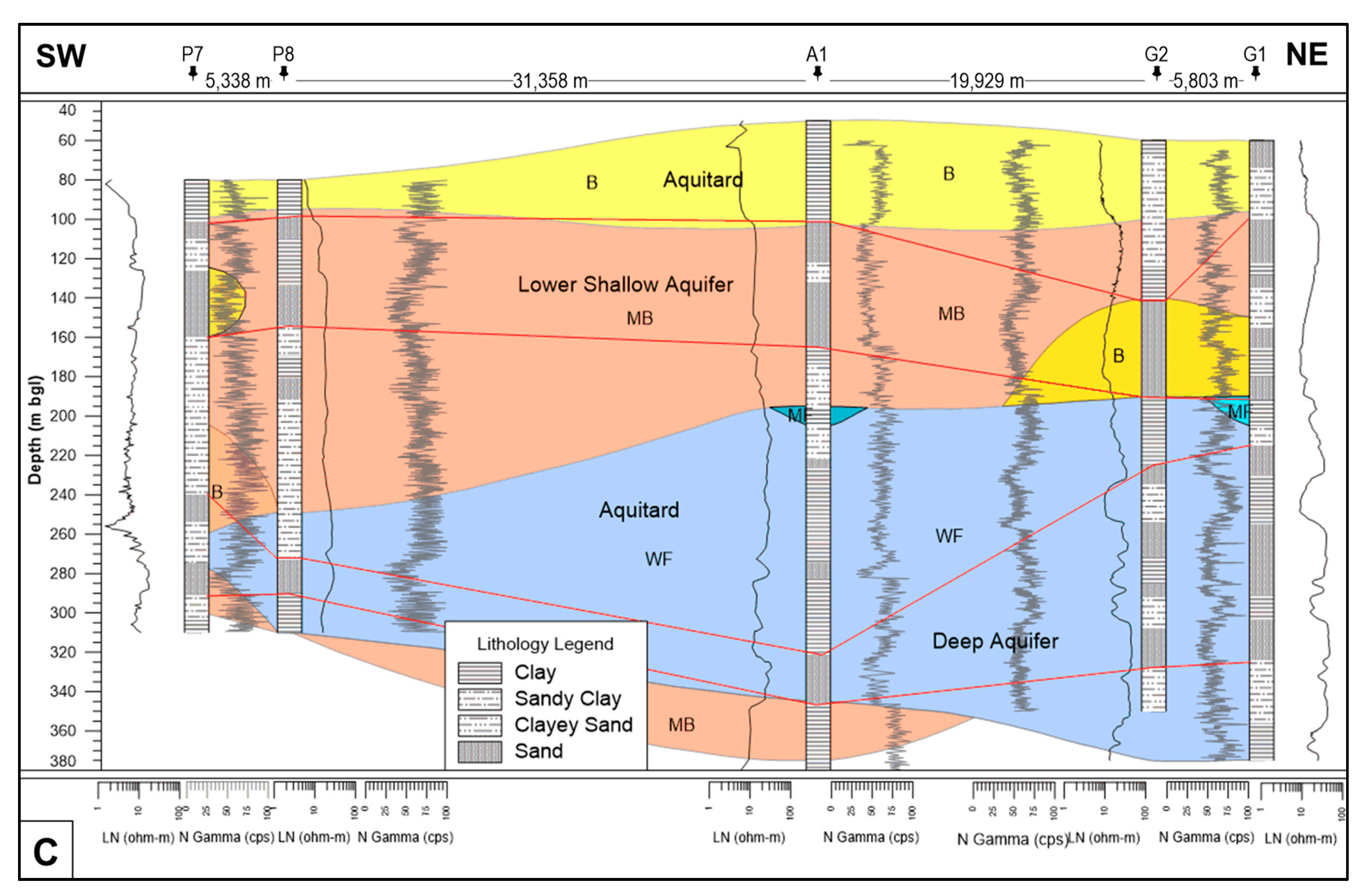
4.1. Geophysical Cross-Section
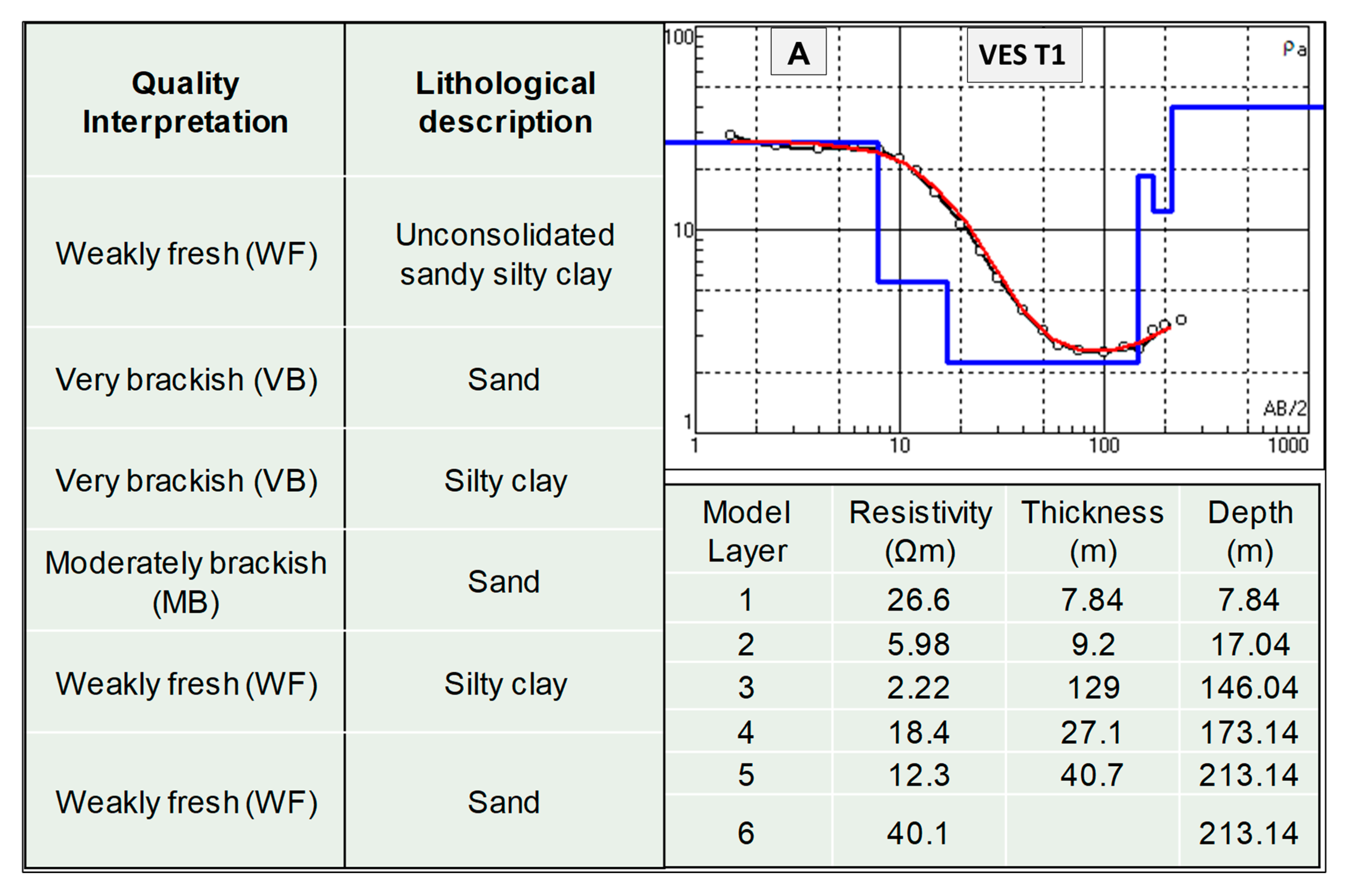
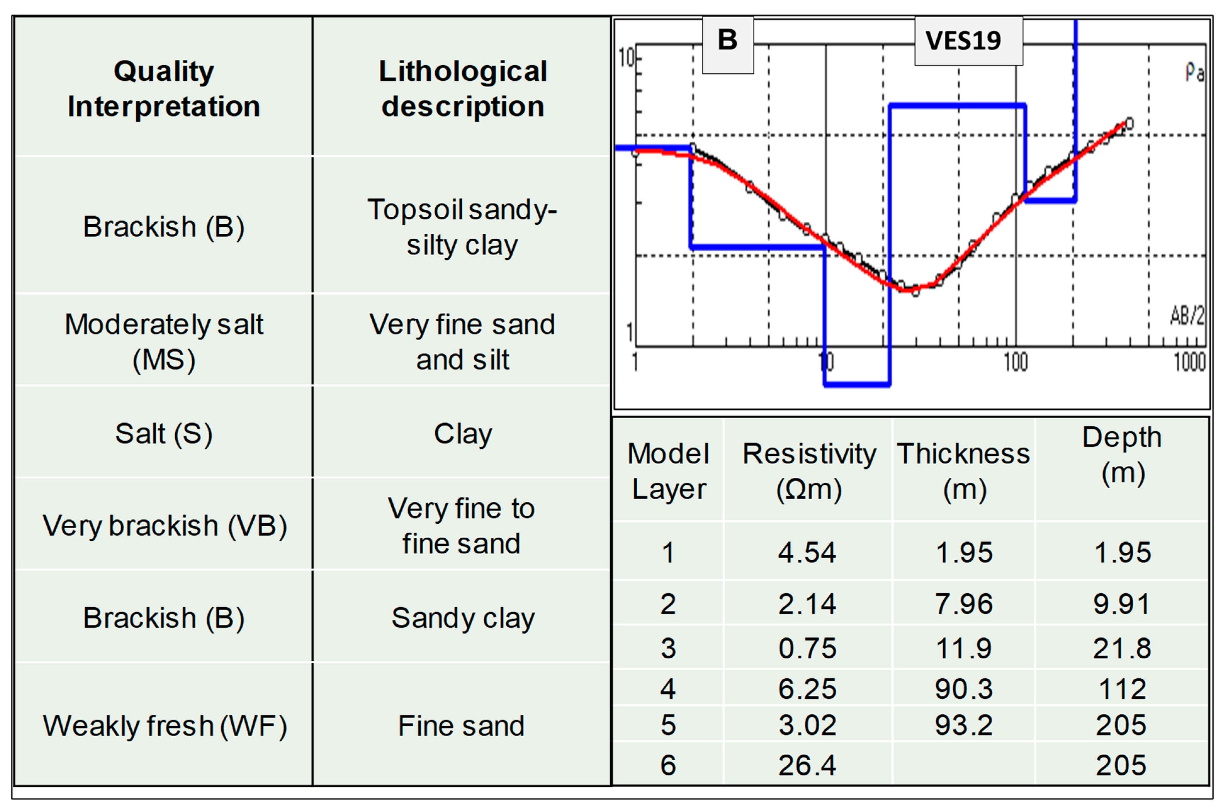
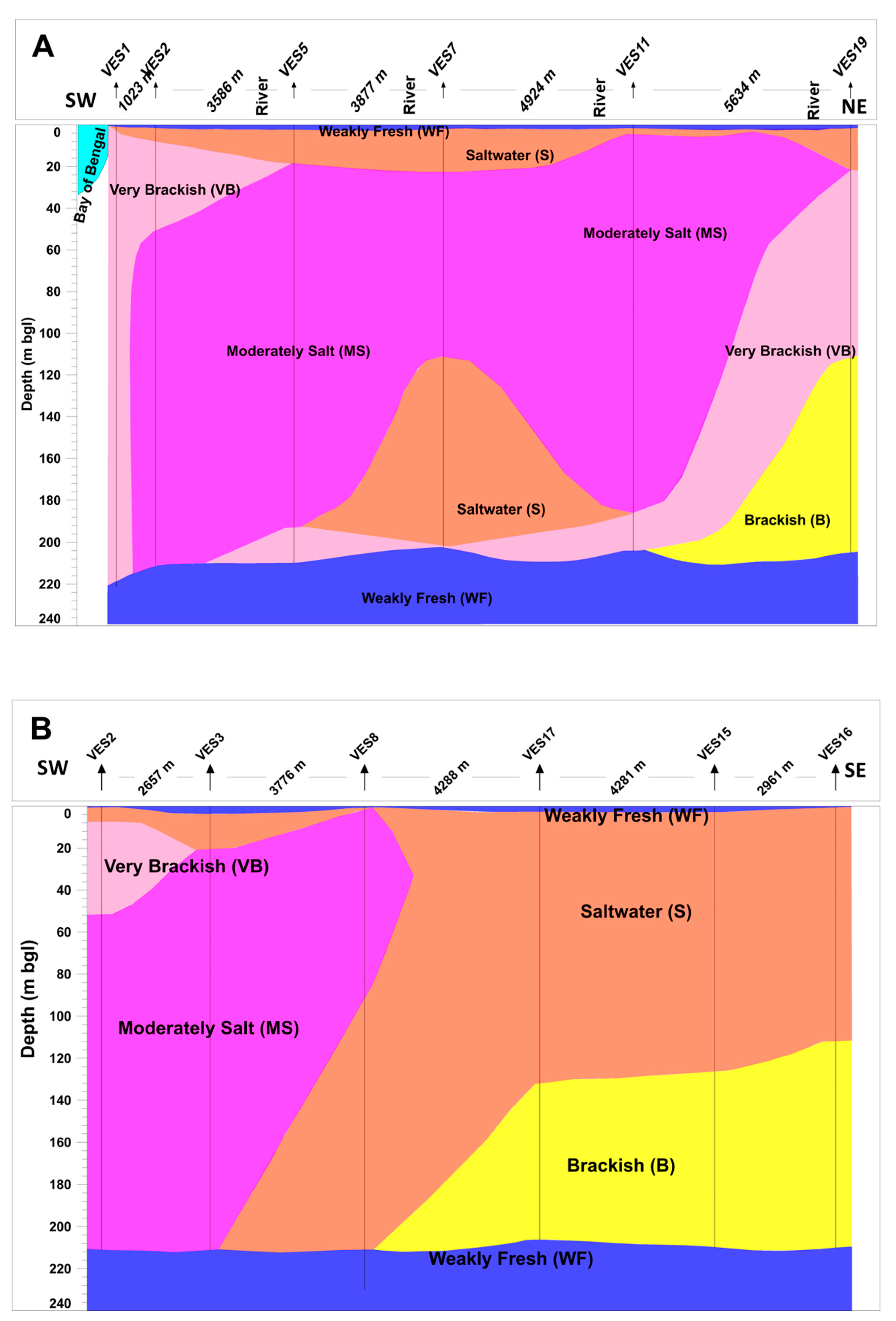
4.2. VES
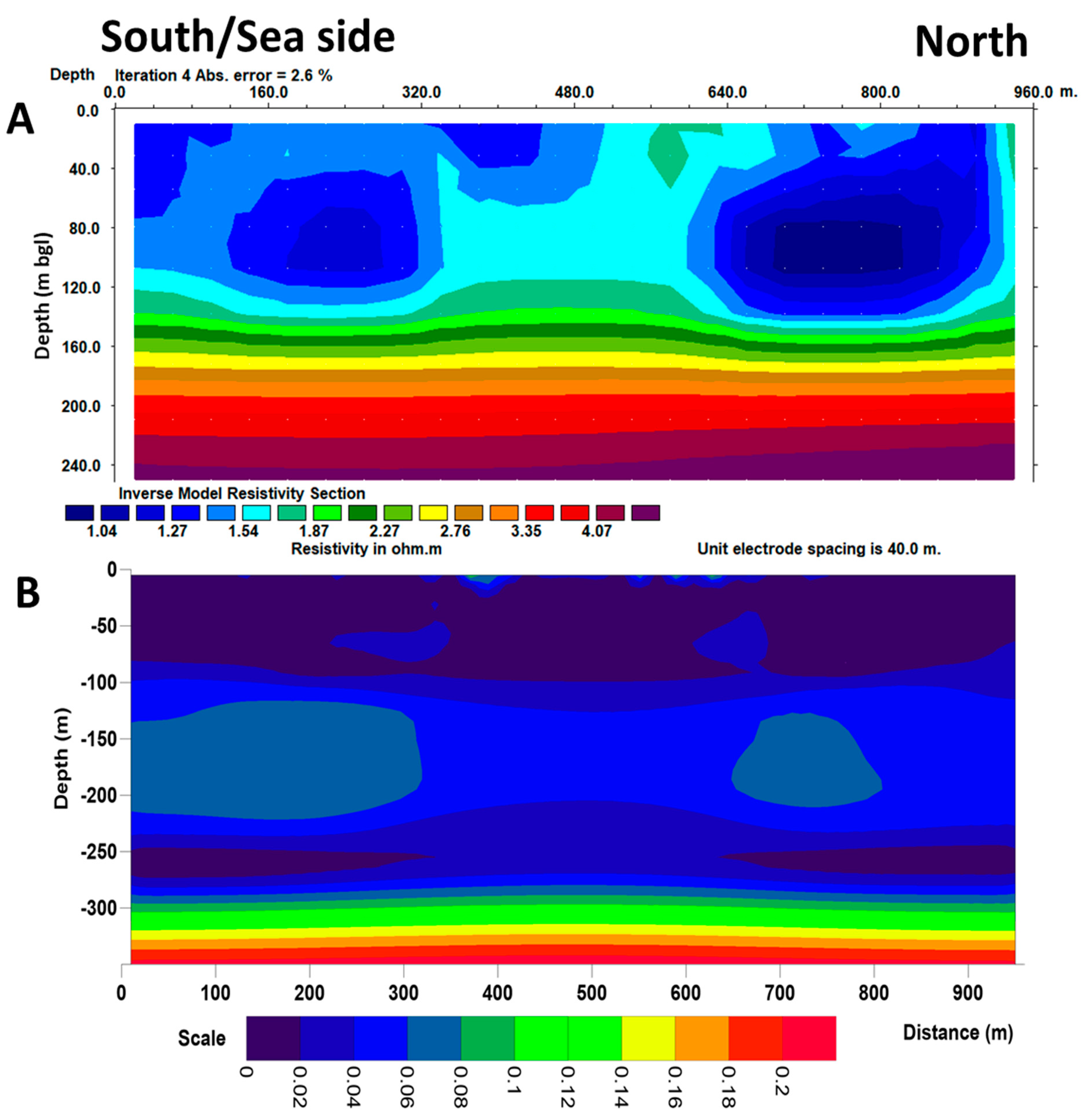
4.3. ERT
5. Discussion
6. Conclusions
Author Contributions
Funding
Institutional Review Board Statement
Informed Consent Statement
Data Availability Statement
Acknowledgments
Conflicts of Interest
References
- Karim, Z. Salinity Problems and Crop Intensification in the Coastal Regions of Bangladesh. Soil Publ. No. 33, 1990. Available online: https://www.researchgate.net/publication/264419412_Salinity_Problems_and_Crop_Intensification_in_the_Coastal_Regions_of_Bangladesh (accessed on 1 June 2021).
- United Nations Children’s Fund (UNICEF), Bangladesh MICS 2012-2013: Water Quality Thematic Report. Government of Bangladesh, Bangladesh Bureau of Statistics, and UNICEF, 2018. Available online: https://www.unicef.org/bangladesh/sites/unicef.org.bangladesh/files/2018-10/Drinking%20Water%20Quality%20in%20Bangladesh.pdf (accessed on 1 June 2021).
- Kamruzzaman, A.; Ahmed, F. Study of Performance of Existing Pond Sand Filters in Different Parts of Bangladesh. In Proceedings of the 32nd WEDC International Conference, Colombo, Sri Lanka, 13–17 September 2006; Available online: https://hdl.handle.net/2134/29649 (accessed on 1 June 2021).
- Islam, M.; Chou, F.F.; Kabir, M.R.; Liaw, C.H. Rainwater: A Potential Alternative Source for Scarce Safe Drinking and Arsenic Contaminated Water in Bangladesh. Water Resour. Manag. 2010, 24, 3987–4008. [Google Scholar] [CrossRef]
- Abedin, A.; Habiba, U.; Shaw, R. Community Perception and Adaptation to Safe Drinking Water Scarcity: Salinity, Arsenic, and Drought Risks in Coastal Bangladesh. Int. J. Disaster Risk Sci. 2014, 5, 110–124. [Google Scholar] [CrossRef]
- Khan, A.E.; Ireson, A.; Kovats, S.; Mojumder, S.K.; Khusru, A.; Rahman, A.; Vineis, P. Drinking Water Salinity and Maternal Health in Coastal Bangladesh: Implications of Climate Change. Environ. Health Perspect. 2011, 119, 1328–1332. [Google Scholar] [CrossRef] [PubMed]
- Khan, A.E.; Scheelbeek, P.F.D.; Shilpi, A.B.; Chan, Q.; Mojumder, S.K.; Rahman, A.; Haines, A.; Vineis, P. Salinity in Drinking Water and the Risk of (Pre)Eclampsia and Gestational Hypertension in Coastal Bangladesh: A Case-Control Study. PLoS ONE 2014, 9, e108715. [Google Scholar] [CrossRef] [Green Version]
- Alam, A.; Rahman, M.; Islam, S. Performance of modified design pond sand filters. J. Water Supply Res. Technol.-Aqua 2011, 60, 311–318. [Google Scholar] [CrossRef]
- Sarkar, B.; Islam, A.; Majumder, A. Seawater intrusion into groundwater and its impact on irrigation and agriculture: Evidence from the coastal region of West Bengal, India. Reg. Stud. Mar. Sci. 2021, 44, 101751. [Google Scholar] [CrossRef]
- Barlow, P.M. Ground Water in Freshwater-Saltwater Environments of the Atlantic Coast; Geological Survey (USGS): Sunrise Valley Drive, Reston, VA, USA, 2003; Volume 1262. [Google Scholar] [CrossRef] [Green Version]
- Meisler, H.; Leahy, P.P.; Knobel, L.L. Effect of Eusta108715tic Sea-Level Changes on Saltwater-Freshwater Relations in the Northern Atlantic Coastal Plain; US Government Printing Office: Washington, DC, USA, 1984; Volume 2255. [Google Scholar]
- Jimoh, R.A.; Bankole, O.M.; Ahmed, K.; Christopher, O.A.; Adeniji, M.A.; Ebhodaghe, J.; Sedara, S.O.; Obende, P.W.; Alebu, O.; Ezima, E.A. Use of geophysical logs in hydrogeological studies and borehole designs: Case study of Apapa coastal area, Lagos, Nigeria. Appl. Water Sci. 2018, 8, 191. [Google Scholar] [CrossRef] [Green Version]
- Van Camp, M.; Mtoni, Y.; Mjemah, I.C.; Bakundukize, C.; Walraevens, K. Investigating seawater intrusion due to groundwater pumping with schematic model simulations: The example of the Dar es Salaam coastal aquifer in Tanzania. J. Afr. Earth Sci. 2014, 96, 71–78. [Google Scholar] [CrossRef]
- Walraevens, K.; Mjemah, I.C.; Mtoni, Y.; Van Camp, M. Sources of salinity and urban pollution in the Quaternary sand aquifers of Dar es Salaam, Tanzania. J. Afr. Earth Sci. 2015, 102, 149–165. [Google Scholar] [CrossRef]
- Abedin, M.; Habiba, U.; Shaw, R. Chapter 10 Health: Impacts of Salinity, Arsenic and Drought in South-western Bangladesh; Emerald Group Publishing Limited: Bingley, UK, 2012; pp. 165–193. [Google Scholar] [CrossRef]
- Woobaidullah, A.; Rahman, M.; Romer, A.; Arndt, R. Geoelectric resistivity survey for suitable freshwater aquifer identification in the coastal Belt of south-west Bangladesh. Jb Geol BA 1996, 139, 127–137. [Google Scholar]
- Afroza, R.; Mazumder, Q.H.; Jahan, C.S.; Kazi, M.A.I.; Ahsan, M.A.; Al-Mansur, M.A. Hydrochemistry and origin of salinity in groundwater in parts of Lower Tista Floodplain, northwest Bangladesh. J. Geol. Soc. India 2009, 74, 223–232. [Google Scholar] [CrossRef]
- Aggarwal, P.K.; Froehlich, K.; Basu, A.; Poreda, R.; Kulkarni, K.; Tarafdar, S.; Mohamed, A.; Nasir, A.; Alamgir, H.; Mizanur, R. A Report on Isotope Hydrology of Groundwater in Bangladesh: Implications for Characterization and Mitigation of Arsenic in Groundwater; International Atomic Energy Agency: Vienna, Austria, 2000; 61p. [Google Scholar]
- Bahar, M.M.; Reza, M.S. Hydrochemical characteristics and quality assessment of shallow groundwater in a coastal area of Southwest Bangladesh. Environ. Earth Sci. 2010, 61, 1065–1073. [Google Scholar] [CrossRef]
- Hassan, M.Q. Hydrochemistry of lowlands water of southwest Bangladesh. Lowl. Technol. Int. Off J. Int. Assoc. Lowl. Technol. 2000, 2, 15–22. [Google Scholar]
- Rahman, T.; Mirza, A.; Rahman, S.H.; Majumder, R.K. Groundwater quality for irrigation of deep aquifer in southwestern zone of Banglades. Songklanakarin J. Sci. Technol. 2012, 34. [Google Scholar]
- Sarker, M.R.; van Camp, M.; Islam, M.; Ahmed, N.; Walraevens, K. Hydrochemistry in coastal aquifer of southwest Bangladesh: Origin of salinity. Environ. Earth Sci. 2018, 77, 39. [Google Scholar] [CrossRef]
- Melloul, A.; Goldenberg, L. Monitoring of Seawater Intrusion in Coastal Aquifers: Basics and Local Concerns. J. Environ. Manag. 1997, 51, 73–86. [Google Scholar] [CrossRef] [Green Version]
- Archie, G.E. The Electrical Resistivity Log as an Aid in Determining Some Reservoir Characteristics. Trans. AIME 1942, 146, 54–62. [Google Scholar] [CrossRef]
- Buckley, D.K. Some case histories of geophysical downhole logging to examine borehole site and regional groundwater movement in Celtic regions. Geol. Soc. Lond. Spéc. Publ. 2000, 182, 219–237. [Google Scholar] [CrossRef]
- Buckley, D.K.; Hinsby, K.; Manzano, M. Application of geophysical borehole logging techniques to examine coastal aquifer palaeohydrogeology. Geol. Soc. Lond. Spéc. Publ. 2001, 189, 251–270. [Google Scholar] [CrossRef]
- Hallenburg, J.K. Geophysical Logging for Mineral and Engineering Applications; PennWell Publishing: Tulsa, Oklahoma, 1984. [Google Scholar]
- Mares, S.; Zboril, A.; Kelly, W. Logging for determination of aquifer hydraulic properties. Log Anal. 1994, 35, 28. [Google Scholar]
- Repsold, H. Well logging in groundwater development. Heise 1989, 9, 136. [Google Scholar]
- Cong-Thi, D.; Dieu, L.; Thibaut, R.; Paepen, M.; Ho, H.; Nguyen, F.; Hermans, T. Imaging the Structure and the Saltwater Intrusion Extent of the Luy River Coastal Aquifer (Binh Thuan, Vietnam) Using Electrical Resistivity Tomography. Water 2021, 13, 1743. [Google Scholar] [CrossRef]
- Bangladesh Bureau of Statistics (BBS). Statistical Yearbook of Bangladesh; Bangladesh Bureau of Statistics, Ministry of Planning: Dhaka, Bangladesh, 2005. [Google Scholar]
- Website. Available online: http://www.tides4fishing.com/as/bangladesh/sundarban (accessed on 27 May 2021).
- Bangladesh Bureau of Statistics (BBS). Population and Housing Census. In Socio-Economic and Demographic Report, National Series; Ministry of Planning, Statistics and Informatics Division (SID): Dhaka, Bangladesh, 2011; Volume 4. [Google Scholar]
- Cooper, H., Jr.; Jacob, C.E. A generalized graphical method for evaluating formation constants and summarizing well-field history. Eos Trans. Am. Geophys. Union 1946, 27, 526–534. [Google Scholar] [CrossRef]
- Sarker, M.M.R. Hydrogeology and Hydrochemistry in a Coastal Aquifer: A Case Study from Southwestern Part of Bangladesh. Master’s Thesis, Universiteit Brussel and Universiteit Gent, Ghent, Belgium, 2016. [Google Scholar]
- Gheorghe, A. Processing and Synthesis of Hydrogeological Data; Abacus Press: Hachette, UK, 1978. [Google Scholar]
- Ferris, J.G.; Knowles, D.; Brown, R.; Stallman, R.W. Theory of Aquifer Tests; US Government Printing Office: Washington, DC, USA, 1962.
- Hvorslev, M.J. Time Lag and Soil Permeability in Ground-Water Observations; Corps of Engineers, US Army: Washington, DC, USA, 1951. [Google Scholar]
- Kruseman, G.P.; de Ridder, N.A.; Verweij, M.J. Analysis and Evaluation of PumpingTest Data; International Institute for Land Reclamation and Improvement: Wageningen, The Netherlands, 1970; Volume 11. [Google Scholar]
- Boughriba, M.; Melloul, A.; Zarhloule, Y.; Ouardi, A. Extension Spatiale de la Salinisation des Ressources en eau et Modèle Conceptuel des Sources Salées Dans la Plaine des Triffa (Maroc Nord-Oriental). Comptes Rendus Geosci. 2006, 338, 768–774. [Google Scholar] [CrossRef]
- Guasmia, M. Caracterisation de la Geometrie des Aquiferes Alluvionnaires, Neogene Sableux et Cretace Carbonate du Bassin de Gafsa par les Methods Geophysiques. Ph.D. Thesis, Universite de Sfax, Sfax, Tunisia, 2008; 220p. [Google Scholar]
- Adepelumi, A.A.; Ako, B.D.; Ajayi, T.R.; Afolabi, O.; Omotoso, E.J. Delineation of saltwater intrusion into the freshwater aquifer of Lekki Peninsula, Lagos, Nigeria. Environ. Earth Sci. 2008, 56, 927–933. [Google Scholar] [CrossRef]
- Wilson, S.; Ingham, M.; McConchie, J. The applicability of earth resistivity methods for saline interface definition. J. Hydrol. 2006, 316, 301–312. [Google Scholar] [CrossRef]
- Nguyen, F.; Kemna, A.; Antonsson, A.; Engesgaard, P.; Kuras, O.; Ogilvy, R.; Gisbert, J.; Jorreto, S.; Pulido-Bosch, A. Characterization of seawater intrusion using 2D electrical imaging. Near Surf. Geophys. 2009, 7, 377–390. [Google Scholar] [CrossRef] [Green Version]
- Goebel, M.; Pidlisecky, A.; Knight, R. Resistivity imaging reveals complex pattern of saltwater intrusion along Monterey coast. J. Hydrol. 2017, 551, 746–755. [Google Scholar] [CrossRef]
- Keys, W.S. A Practical Guide to Borehole Geophysics in Environmental Investigations; Routledge: London, UK, 2017. [Google Scholar]
- Belknap, W.B.; Dewan, J.T.; Kirkpatrick, C.; Mott, W.E.; Pearson, A.; Rabson, W. API calibration facility for nuclear logs. In Drilling and Production Practice; American Petroleum Institute: Washington, DC, USA, 1959. [Google Scholar]
- Reynolds, J.M. An Introduction to Applied and Environmental Geophysics; John Wiley & Sons: Hoboken, NJ, USA, 2011. [Google Scholar]
- Ministry of Science and Technology (MoST). Government of People’s Republic of Bangladesh, Evaluation and Monitoring the Consequences of Saline Water Intrusion and Land Erosion-Accretion on the South-Central Coastal Ecosystem of Bangladesh; MoST: Dhaka, Bangladesh, 2014–2016. [Google Scholar]
- IPI2WIN-1D Program. In Programs Set for 1D VES Data Interpretation; Moscow University: Moscow, Russia, 2000.
- Tikhonov, A.N.; Arsenin, V.Y. Solutions of ill-posed problems. SIAM Rev. 2012, 21, 266–267. [Google Scholar] [CrossRef]
- Caterina, D.; Hermans, T.; Nguyen, F. Case studies of incorporation of prior information in electrical resistivity tomography: Comparison of different approaches. Near Surf. Geophys. 2014, 12, 451–465. [Google Scholar] [CrossRef] [Green Version]
- Loke, M.; Chambers, J.; Rucker, D.; Kuras, O.; Wilkinson, P. Recent developments in the direct-current geoelectrical imaging method. J. Appl. Geophys. 2013, 95, 135–156. [Google Scholar] [CrossRef]
- Loke, M.; Barker, R. Rapid least-squares inversion of apparent resistivity pseudosections by a quasi-Newton method1. Geophys. Prospect. 1996, 44, 131–152. [Google Scholar] [CrossRef]
- Loke, M. Rapid 2D Resistivity Forward Modeling Using the Finite-Difference and Finite-Element Methods; Geotomo Software: Penang, Malaysia, 2002. [Google Scholar]
- Oldenburg, D.W.; Li, Y. Estimating depth of investigation in dc resistivity and IP surveys. Geophysics 1999, 64, 403–416. [Google Scholar] [CrossRef]
- Caterina, D.; Beaujean, J.; Robert, T.; Nguyen, F. A comparison study of different image appraisal tools for electrical resistivity tomography. Near Surf. Geophys. 2013, 11, 639–658. [Google Scholar] [CrossRef]
- Paepen, M.; Hanssens, D.; Smedt, P.D.; Walraevens, K.; Hermans, T. Combining resistivity and frequency domain electromagnetic methods to investigate submarine groundwater discharge in the littoral zone. Hydrol. Earth Syst. Sci. 2020, 24, 3539–3555. [Google Scholar] [CrossRef]
- Parsekian, A.D.; Claes, N.; Singha, K.; Minsley, B.J.; Carr, B.; Voytek, E.B.; Harmon, R.; Kass, A.; Carey, A.; Thayer, D.; et al. Comparing Measurement Response and Inverted Results of Electrical Resistivity Tomography Instruments. J. Environ. Eng. Geophys. 2017, 22, 249–266. [Google Scholar] [CrossRef]
- Marescot, L.; Loke, M.; Chapellier, D.; Delaloye, R.; Lambiel, C.; Reynard, E. Assessing reliability of 2D resistivity imaging in mountain permafrost studies using the depth of investigation index method. Near Surf. Geophys. 2002, 1, 57–67. [Google Scholar] [CrossRef]
- Patnode, H.; Willie, M. The presence of borehole geophysics to water resources investigations. In Techniques of Waterresources Investigations of the USGS; Book 2; U.S. Geological Survey: Seattle, WA, USA, 1950. [Google Scholar]
- Vlieghe, C. Hydrogeologische Studie van het Poldergebied in de Omgeving van Booitshoeke. Master’s Thesis, Ghent University, Ghent, Belgium, 1994. [Google Scholar]
- de Moor, G.; de Breuck, W. De freatische waters in het Oostelijk Kustgebied en in de Vlaamse Vallei. Natuurwet. Tijdschr. 1969, 51, 3–68. [Google Scholar]
- Walraevens, K.; Lebbe, L.; van Camp, M.; Angius, G.; Serra, M.; Vacca, A.; Massidda, R.; Debreuck, W. Salt fresh-water flow and distribution in a cross-section at Oostduinkerke (Western Coastal-Plain of Belgium). Study Model. Saltwater Intrusion Aquifers 1993, 407–420. [Google Scholar]
- Vandenbohede, A.; Walraevens, K.; de Breuck, W. What does the interface on the fresh-saltwater distribution map of the Belgian coastal plain represent? Geol. Belg. 2015, 18, 31–36. [Google Scholar]
- Sarker, M.M.R.; van Camp, M.; Hossain, D.; Islam, M.; Ahmed, N.; Karim, M.M.; Bhuiyan, M.A.Q.; Walraevens, K. Groundwater salinization and freshening processes in coastal aquifers from southwest Bangladesh. Sci. Total Environ. 2021, 779, 146339. [Google Scholar] [CrossRef] [PubMed]
- Sarker, M.M.R.; Camp, M.V.; Hossain, D.; Islam, M.; Bhuiyan, M.A.Q.; Ahsan, M.A.; Bennett, G.; Walraevens, K. Understanding the Hydrogeochemical Evolution of Groundwater in Coastal Aquifers of Southwest Bangladesh. In Proceedings of the EGU General Assembly Conference Abstracts 2021, online. 19–30 April 2021; EGU21-9767. Available online: https://doi.org/10.5194/egusphere-egu21-9767 (accessed on 1 June 2021).
- Islam, M.; Siddika, A.; Khan, M.; Goldar, M.; Sadique, M.A.; Kabir, A.; Huq, A.; Colwell, R. Microbiological analysis of tube-well water in a rural area of Bangladesh. Appl. Environ. Microbiol. 2001, 67, 3328–3330. [Google Scholar] [CrossRef] [PubMed] [Green Version]
- Faneca Sànchez, M.; Bashar, K.; Janssen, G.; Vogels, M.; Snel, J.; Zhou, Y.; Stuurman, R.J.; Essink, G.O. SWIBANGLA: Managing Salt Water Intrusion Impacts in Coastal Groundwater Systems of Bangladesh. 2015. Available online: https://www.deltares.nl/app/uploads/2015/04/1207671-000-BGS-0016-r-SWIBANGLA-def.pdf (accessed on 1 June 2021).
- Michael, H.A.; Voss, C.I. Controls on groundwater flow in the Bengal Basin of India and Bangladesh: Regional modeling analysis. Hydrogeol. J. 2009, 17, 1561. [Google Scholar] [CrossRef]
- Allison, M.; Khan, S.; Goodbred, S.; Kuehl, S. Stratigraphic evolution of the late Holocene Ganges–Brahmaputra lower delta plain. Sediment. Geol. 2003, 155, 317–342. [Google Scholar] [CrossRef]
- Goodbred, S., Jr.; Kuehl, S.A. The significance of large sediment supply, active tectonism, and eustasy on margin sequence development: Late Quaternary stratigraphy and evolution of the Ganges–Brahmaputra delta. Sediment. Geol. 2000, 133, 227–248. [Google Scholar] [CrossRef]
- Umitsu, M. Late Quaternary sedimentary environment and landform evolution in the Bengal lowland. Geogr. Rev. Jpn. Ser. B 1987, 60, 164–178. [Google Scholar] [CrossRef] [Green Version]
- Umitsu, M. Late quaternary sedimentary environments and landforms in the Ganges Delta. Sediment. Geol. 1993, 83, 177–186. [Google Scholar] [CrossRef]
- Fairbridge, R.W. Eustatic changes in sea level. Phys. Chem. Earth 1961, 4, 99–185. [Google Scholar] [CrossRef]
- Khan, S.R.; Islam, B. Holocene stratigraphy of the lower Ganges-Brahmaputra river delta in Bangladesh. Front. Earth Sci. China 2008, 2, 393–399. [Google Scholar] [CrossRef]


| Resistivity Group | Water Quality Class | Total Dissolved Solids (TDSs) (mg/L) | Pore-Water Resistivity | Formation Resistivity (Clay) Equation (5) | Formation Resistivity (Sand) |
|---|---|---|---|---|---|
| VF | Very fresh | <200 | >50 | >33.33 | >200 |
| F | Fresh | 200–400 | 50–25 | 33.33–25 | 200–100 |
| MF | Moderately fresh | 400–800 | 25–12.5 | 25–16.66 | 100–50 |
| WF | Weakly fresh | 800–1600 | 12.5–6.25 | 16.66–10 | 50–25 |
| MB | Moderately brackish | 1600–3200 | 6.25–3.13 | 10–5.56 | 25–12.5 |
| B | Brackish | 3200–6400 | 3.13–1.56 | 5.56–2.93 | 12.5–6.25 |
| VB | Very brackish | 6400–12,800 | 1.56–0.78 | 2.93–1.51 | 6.25–3.12 |
| MS | Moderately salt | 12,800–25,600 | 0.78–0.39 | 1.51–0.76 | 3.12–1.56 |
| S | Salt | >25,600 | <0.39 | <0.76 | <1.56 |
Publisher’s Note: MDPI stays neutral with regard to jurisdictional claims in published maps and institutional affiliations. |
© 2021 by the authors. Licensee MDPI, Basel, Switzerland. This article is an open access article distributed under the terms and conditions of the Creative Commons Attribution (CC BY) license (https://creativecommons.org/licenses/by/4.0/).
Share and Cite
Sarker, M.M.R.; Van Camp, M.; Hermans, T.; Hossain, D.; Islam, M.; Uddin, M.Z.; Ahmed, N.; Bhuiyan, M.A.Q.; Karim, M.M.; Walraevens, K. Geophysical Delineation of Freshwater–Saline Water Interfaces in Coastal Area of Southwest Bangladesh. Water 2021, 13, 2527. https://doi.org/10.3390/w13182527
Sarker MMR, Van Camp M, Hermans T, Hossain D, Islam M, Uddin MZ, Ahmed N, Bhuiyan MAQ, Karim MM, Walraevens K. Geophysical Delineation of Freshwater–Saline Water Interfaces in Coastal Area of Southwest Bangladesh. Water. 2021; 13(18):2527. https://doi.org/10.3390/w13182527
Chicago/Turabian StyleSarker, Md. Mizanur Rahman, Marc Van Camp, Thomas Hermans, Delwar Hossain, Mazeda Islam, Mohammad Zohir Uddin, Nasir Ahmed, Md. Abdul Quaiyum Bhuiyan, Md. Masud Karim, and Kristine Walraevens. 2021. "Geophysical Delineation of Freshwater–Saline Water Interfaces in Coastal Area of Southwest Bangladesh" Water 13, no. 18: 2527. https://doi.org/10.3390/w13182527
APA StyleSarker, M. M. R., Van Camp, M., Hermans, T., Hossain, D., Islam, M., Uddin, M. Z., Ahmed, N., Bhuiyan, M. A. Q., Karim, M. M., & Walraevens, K. (2021). Geophysical Delineation of Freshwater–Saline Water Interfaces in Coastal Area of Southwest Bangladesh. Water, 13(18), 2527. https://doi.org/10.3390/w13182527