Remote Retrieval of Suspended Particulate Matter in Inland Waters: Image-Based or Physical Atmospheric Correction Models?

Abstract

The objective of this paper was to compare the limits of three image-based atmospheric correction models (top of the atmosphere (ToA), dark object subtraction (DOS), and cosine of the sun zenith angle (COST)), and three physical models (atmospheric correction for flat terrain (ATCOR), fast line-of-sight atmospheric analysis of spectral hypercubes (FLAASH)), and ACOLITE) for retrieving suspended particulate matter (SPM) concentrations in inland water bodies using Landsat imagery. For SPM concentration estimates, all possible combinations of 2-band normalized ratios ($2b_{NR}$) were computed, and a stepwise regression was applied. The correlation analysis allowed highlighting that the red/blue $2b_{NR}$ was the best spectral index to retrieve SPM concentrations in the case of image-based models, while the red/green $2b_{NR}$ was the best in the case of physical models. Contrary to expectations, image-based atmospheric models outperformed the accuracy of physical models. The cross-validation results underlined the good performance of the DOS and COST models, with R² > 0.83, NASH-criterion (Nash) > 0.83, bias = −0.01 mg/L, and RMSE < 0.27 mg/L. This outperformance was confirmed using blind test validation data, with an R² > 0.86 and Nash > 0.58 for the DOS and COST models. The challenges and limitations involved in the remote monitoring of SPM spatial distribution in turbid productive waters using satellite data are discussed at the end of the paper.

1. Introduction

Suspended particulate matter (SPM) is an important element for water quality evaluations [1] and plays a major role in the ecological regulation of aquatic systems [2]. SPM is an indicator of water turbidity [3] that can be of minerals, humic, or planktonic origin and can be considered as a stimulating factor for cyanobacteria bloom growth [2,4]. Indeed, a part of the sunlight’s ultraviolet wavelengths are backscattered by SPM, which both favors the increase of bacteria and decreases their mortality [5]. Such conditions are ideal for the development of cyanobacteria, and once established, they are very difficult to control and to mitigate [6]. Lakes experiencing recurrent cyanobacteria are subject to an accelerated eutrophication, and their water can be a real threat to human and animal health [7,8,9], since some species are toxin-carrying.

In situ sampling is the most accurate and commonly used technique to monitor SPM concentrations, but it is costly and limited in time and space for representative lake water quality characterization. The SPM in lakes causes distinct changes in the water color by absorbing and scattering the sunlight at specific spectral wavelengths. This physical behavior can be used to retrieve SPM concentrations based on the reflectance of remotely sensed data, by relating optical changes observed in these specific spectral wavelengths to in situ measurements of SPM concentration.

Based on this principle, several empirical models [4,10,11,12,13,14] were developed, and they were able to estimate SPM concentrations using many sensor types (MERIS, MODIS, SPOT, Landsat, and Sentinel-2). However, estimation accuracy has often been moderate. Numerous authors have reported this issue and have related it to atmospheric correction using physical models, which were not initially designed for inland waters applications [14,15,16]. Furthermore, the analysis made by Wang, Chen [17], which aimed to compare more than 20 algorithms used for retrieving SPM concentration using Landsat images corrected by the 6S model (second simulation of a satellite signal in the solar spectrum) also emphasized the lack of SPM estimate accuracy (R² < 0.78).

Indeed, up to 80% of remotely sensed signals recorded by sensors are backscattered by the air column of the atmosphere and do not represent the real optical feature of interest [18]. Unlike open oceans (known as case-1 waters), the optical properties of inland waters (known as case-2 waters) are very complex [19]. In addition to the SPM, there are many other optically active components (chlorophyll-a of phytoplankton (chl_a) and colored dissolved organic matter (CDOM), among others) that render SPM modeling very challenging in these aquatic systems [20]. A poor atmospheric correction could thus lead to significant errors in estimating the reflectance and affect the accuracy of SPM modeling [21].

In fact, researchers have subdivided the effect of the atmosphere on sun-light radiance into two groups: a multiplicative effect that is caused by the aerosol optical depth at 550 nm, ozone, and transmittance; and an additive effect that is mainly caused by haze [22,23,24]. Physical models implemented in most industrial software (atmospheric correction for flat terrain (ATCOR) in PCI-Geomatics and fast line-of-sight atmospheric analysis of spectral hypercubes (FLAASH) in ENVI, for instance) were developed to correct both multiplicative and additive atmospheric effects, but are based on the 0 water-leaving radiance assumption in the near infrared (NIR), which is incorrect for case-2 waters. Therefore, their use is usually error-tainted, specifically in the case of turbid waters [25,26]. As a solution, a new algorithm, called ACOLITE, was recently developed for water applications that is based on the 0 water-leaving radiance assumption in the short wave of infrared (SWIR) [27]. Image-based models (apparent reflectance at the top of the atmosphere (ToA), dark object subtraction (DOS), and cosine of the sun zenith angle (COST), for instance), on the other hand, only correct for the additive effect. This correction consists of subtracting the extra energy caused by the atmosphere for features that are dark, assuming that they should have a reflectance of 1%. Of course, the images are partially corrected and are still tainted by the multiplicative effect, but the original signal recorded by the images is barely modified and preserves its initial optical properties.

Thus, the aim of this work was to test whether complex physical model corrections on spectra are to the advantage of SPM modeling in inland water bodies or whether minimal corrections to spectra using image-based models yield the best results. To do so, a comparative analysis was performed between three physical models (ATCOR, FLAASH, and ACOLITE) and three image-based models (ToA, DOS, and COST) to evaluate the accuracy of SPM modeling over two inland water bodies using Landsat images. Models were calibrated using a stepwise multivariate regression and were evaluated using the cross-validation technique and a blind test database. For the accuracy assessment, four statistical indices were used (coefficient of determination (R²), root mean square error (RMSE), bias, and NASH-criterion (Nash)).

2. Materials and Methods

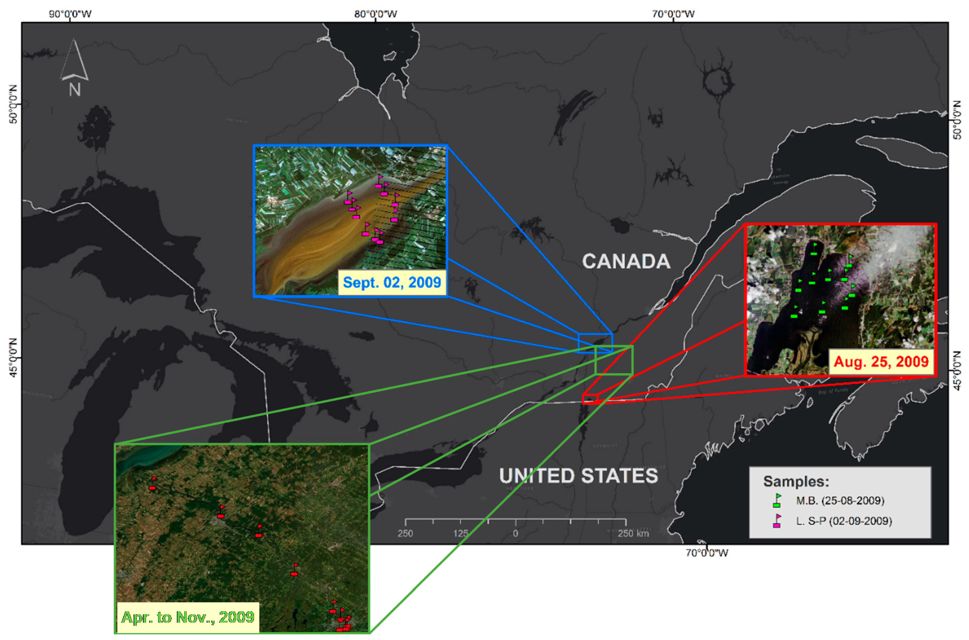
2.1. Calibration and Cross-Validation Database

The data used in this study were collected from two water bodies (Missisquoi Bay (M.B.) of Champlain Lake and Lake Saint-Pierre (St-P.)) known to be turbid in the Québec Province. M.B. of Champlain Lake is located in the northern end (southern part of the province of Quebec) of the lake in the Lake Champlain Valley, on the border of the states of Vermont and New York. The lake area is 1269 km² and its watershed is 23,720 km². The length and width are 201 and 23 km respectively, and the maximum depth is 122 m. The St-P. Lake is located on the St. Lawrence River, between Sorel-Tracy and Trois-Rivières, in Quebec, Canada. The lake is located downstream and east of Montreal, and upstream and west of Quebec City. The lake area is 353 km² and its watershed is 990,000 km². The length and width are 35 and 10 km, respectively, and maximum depth is 20 to 11 m.

In situ analyses were made for physical nutriments (SPM, Chlorophyll-a (chl_a), dissolved organic carbon (DOC), total organic carbon (TOC), total nitrogen (TN), and total phosphorus (TP)). Samples were collected over three years (2008 to 2010) for a total of 769 samples. Only two sampling dates matched with the Landsat sensor’s cross-pass over the two studied water bodies (25 August 2009, for M.B. of Champlain Lake, and 2 September 2009, for St-P. Lake) for a total of 20 samples. However, due to the cloud coverage over M.B. of Champlain Lake (red zoom on Figure 1) and the lack laboratory results for some samples, three additional measures were removed, reducing the size of the calibration database to 17 samples, with a maximum, minimum, mean, and standard deviation of: 40.2, 2.8, 10.75, and 8.22 mg/L for St-P, and 12.3, 1.6, 4.77, and 2.15 mg/L for M.B. (

Table 1. Descriptive statistics of the parameters measured over Missisquoi Bay (M.B.) of Champlain Lake (red zoom (Figure 1)) and Lake Saint-Pierre (St-P (blue zoom (Figure 1))) for the three studied years (2008–2010). Values marked in red bold refer to database statistics used in this study.

Parameters	2008		2009		2010
	M.B. Mean ± Std (min–max)	St-P. Mean ±Std (min–max)	M.B. Mean ± Std (min–max)	St-P. Mean ± Std (min–max)	M.B. Mean ± Std (min–max)	St-P. Mean ± Std (min–max)
SPM (mg/L)	3.94 ± 2.12 (2.10–9.30)	–	4.77 ± 2.15 (1.60–12.30)	10.75 ± 8.22 (2.80–40.20)	13.12 ± 9.17 (7.80–51.20)	–
chl_a (µg/L)	7.80 ± 6.68 (3.30–26.41)	–	13.28 ± 8.51 (5.00–51.05)	6.16 ± 10.43 (1.47–63.71)	23.65 ± 7.88 (4.37–34.21)	–
DOC (mg C/L)	4.72 ± 0.61 (4.38–6.61)	–	4.77 ± 0.20 (4.40–5.12)	4.69 ± 1.61 (2.46–7.43)	6.91 ± 0.68 (5.40–8.53)	–
TOC (mg C/L)	–	–	4.88 ± 0.19 (4.45–5.40)	4.80 ± 1.68 (2.57–7.96)	7.43 ± 0.65 (5.66–8.61)	–
TN (mg N/L)	–	–	–	–	0.84 ± 0.18 (0.55–1.51)	–
TP (mn P/L)	–	–	0.05 ± 0.01 (0.03–0.07)	0.03 ± 0.03 (0.01–0.08)	0.07 ± 0.01 (0.05–0.09)	–

).

2.2. Validation Test Database

In order to test the performance of the SPM modeling, a blind test validation database was used. These data are freely available at the COGESAF (Conseil de gouvernance de l’eau des bassins versants de la rivière Saint-François) web-server (http://cogesaf.sigmont.org/cogesaf/cogesaf.php, accessed date 11 July 2021). Since 2000, COGESAF has been working with sampling results to monitor water quality in the Saint-Francis (St-F.) river watershed. Water parameters such as SPM and phosphorus, among others, are constantly measured in the rivers belonging to this watershed. However, only the annual medians are uploaded to the server. The St-F. River is 200 km long and has an average width of 2.5 km. Data collected from nine stations (green frame of Figure 1) located on the St-F. River were used in this testing process, with a maximum, minimum, mean, and standard deviation of: 10.00, 2.50, 5.22, and 2.29 mg/L per annual median. Since the in situ SPM data are annual medians, it was necessary to compute annual medians of remotely estimated SPM concentrations as well. Thus, cloud-free Landsat images from April to November, 2009 (N = 12) were used for this purpose.

2.3. Image Pre-Processing

Six different models were used to atmospherically correct the two Landsat images: three physical models and three image-based models.

2.3.1. Atmospheric Correction for Flat Terrain (ATCOR)

ATCOR is an approach based on physical data developed by Richter [28]. It aims to minimize atmospheric and illumination effects on high spatial resolution satellite sensors to retrieve physical parameters of the Earth’s surface, such as atmospheric conditions (emissivity and temperature), thermal, and atmospheric radiance (https://www.satimagingcorp.com/services/atcor/, accessed date 15 July 2020). The ATCOR model has several sub-models (ATCOR-2, ATCOR-3, ATCOR-4, and ATCOR Thermal). Each is optimized for specific conditions (flat terrain, mountainous terrain, airborne remotely sensed images, and correction for thermal images, respectively [29]). This algorithm is implemented in commercial software such as ERDAS Imagine and PCI Geomatics.

2.3.2. Fast Line-of-Sight Atmospheric Analysis of Spectral Hypercubes (FLAASH)

FLAASH is an approach based on physical data developed by Anderson, Felde [30]. It is a sophisticated atmospheric correction model based on the MODTRAN algorithm of radiative transfer. The model considers the radiance reflected from the surface of the Earth and scattered by the atmosphere towards the sensor. The difference between these two radiances is due to the adjacency effect (spatial mixture of radiance among nearby pixels) caused by atmospheric scattering. This algorithm is implemented in ENVI software.

2.3.3. ACOLITE

The ACOLITE is an approach initially developed by Vanhellemont and Ruddick (2014). It is a model designed for aquatic remote sensing applications. In general, the algorithm performs in two steps: (1) correction for the Rayleigh scattering using a look-up table generated using the 6S model (Kotchenova, Vermote [31]), and (2) correction for aerosol based on the assumption of the 0 water-leaving radiance in the SWIR and an exponential spectrum for multiple scattering aerosol reflectance. For this study, an improved version of this algorithm was used. The improvement was in the use of the dark spectrum fitting method instead of the exponential spectrum, which allows selecting the most appropriate band automatically and, hence, avoids amplification of glint and adjacency effects in the atmospheric correction. The ACOLITE model is compiled on Python GUI, which is freely available at: https://odnature.naturalsciences.be/remsem/software-and-data/acolite, accessed date 15 July 2020.

2.3.4. Apparent Reflectance at the Top of Atmosphere (ToA)

The ToA is an image-based approach inspired by the general equation of spectral reflectance proposed by Moran, Jackson [32]. It allows converting the digital number (DN) of images into reflectance using radiance computation. It is not a real atmospheric correction model, since it computes the reflectance captured at the top of the atmosphere, hence the word “apparent”. This algorithm is implemented in most commercial software. It is also available in open-source software such as QGIS and coded in packages in R, Python, and MATLAB.

2.3.5. Dark Object Subtraction (DOS)

DOS is an image-based approach developed by Chavez Jr [33]. It aims to minimize the additive effect of the atmosphere caused by haze. The main assumption is that dark objects should represent 1% of reflectance. The amount of added energy in these pixels is caused by haze. Dark objects within the image are identified by an area with clear water in deep lakes or by the histogram method, which selects the DN of haze from the DN frequency histogram of a digital image. This algorithm is implemented in most commercial software. It is also available in open-source software such as QGIS, as well as being coded in packages such as R, Python, and MATLAB.

2.3.6. Cosine of the Sun Zenith Angle (COST)

COST is an image-based approach and is an enhanced version of DOS. In addition to the additive effect correction, like the one used for the DOS algorithm, COST uses an additional correction for transmittance along the path from the ground toward the sensor (known as TAUz). The correction of this module, which is part of the multiplicative effect of the atmosphere, is made by the computation of the cosine of the solar zenith angle. According to Chavez [34], the solar zenith angle cosine is a good approximation of TAUz. This algorithm is also implemented in most commercial software and coded in the R, Python, and MATLAB packages.

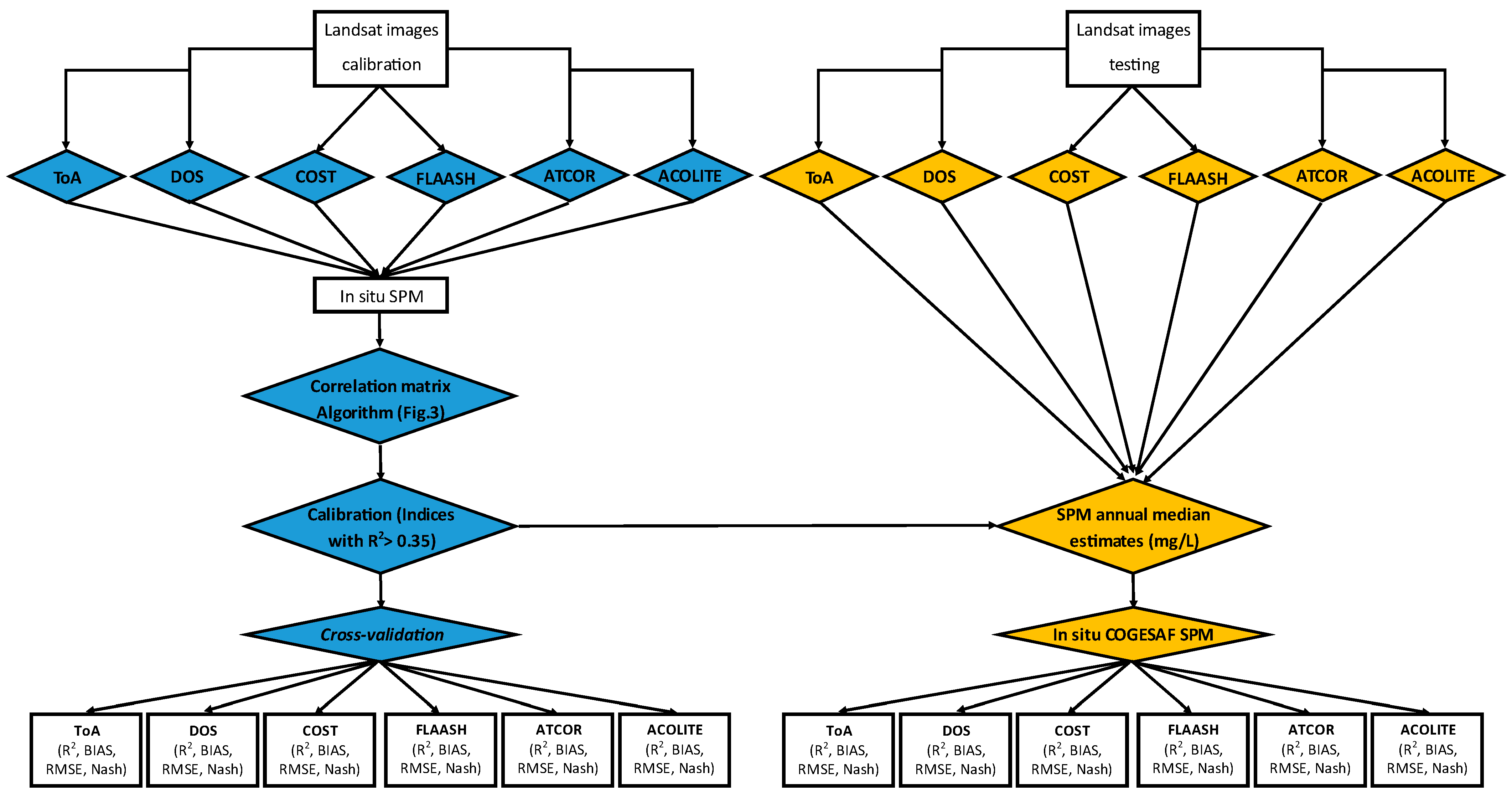
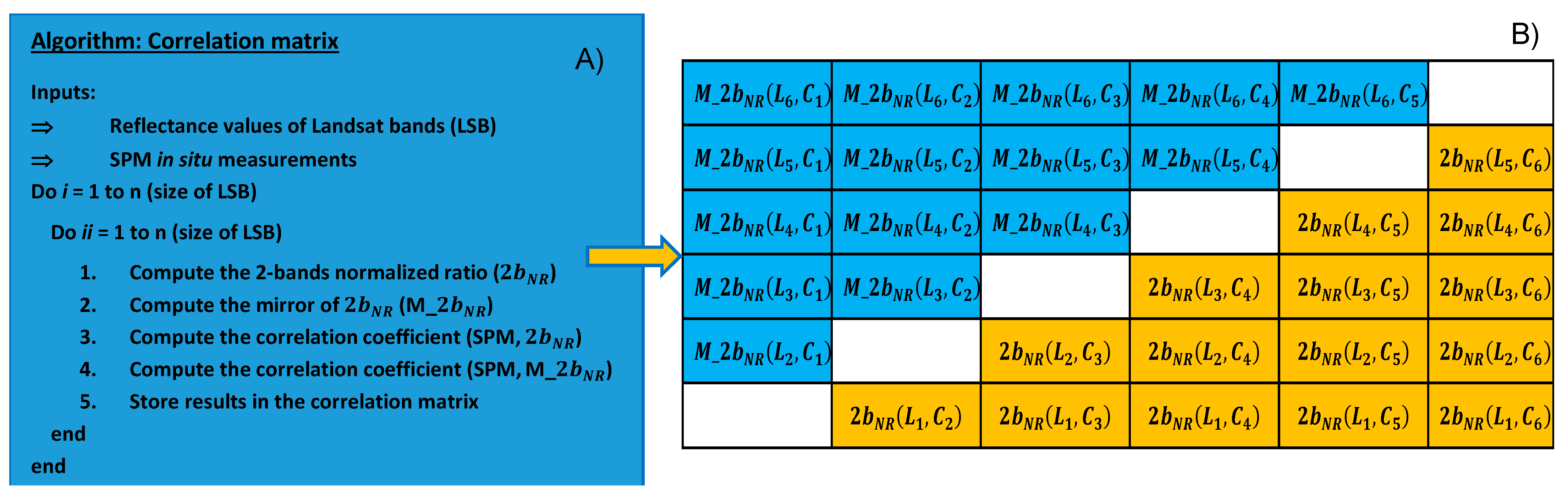
2.4. Methodological Approach and Evaluation Indices

The flowchart in Figure 2 summarizes the methodological steps adopted in this study. After preprocessing images using the six atmospheric correction models, a correlation coefficient matrix (CCM) of all possible combinations of the 2-band normalized ratios ($2b_{NR}$) was calculated (Figure 3) (band ratios and subtractions were also tested; the normalized ratios performed the best). Correlation coefficients were computed based on a simple regression (both linear and exponential correlations were tested; the exponential function fit the best.) between the $2b_{NR}$ indices and in situ measurements of SPM. The $2b_{NR}$ indices for which the R² was higher than 0.35 and were orthogonal one to another were thereafter selected and used in a stepwise multivariate regression for the last calibration. This step reduces the collinearity among the variables ($2b_{NR}$ indices) selected by the stepwise algorithm (blue lozenge in Figure 2).

Due to the reduced size of the database (N = 17), the cross-validation technique was favored. This method involves temporarily removing a given value of SPM from the calibration database and using the remaining observations as a sub-calibration group to estimate the withdrawn value. This operation is repeated for every sample in the database. To assess the accuracy of the modeling, each measured SPM sample is compared to its corresponding estimate using statistical evaluation indices.

For performance analysis with the blind test validation database, Landsat images from April to November 2009 (open water period) over the St-F. River were corrected using the different atmospheric correction models used in this study. Afterwards, the corresponding calibration functions were applied for SPM concentration estimation. The annual medians were thereafter calculated and challenged with the in situ COGESAF data, using the same statistical evaluation indices (orange lozenge in Figure 2).

An example of the computing of the $2b_{NR}$ and its mirror is presented below:

$$2b_{NR}\left(L_i,C_{ii}\right)=\frac{R_s\left({\lambda }_A\right)-R_s\left({\lambda }_B\right)}{R_s\left({\lambda }_A\right)+R_s\left({\lambda }_B\right)}$$

$$M\_2b_{NR}\left(L_{ii},C_i\right)=\frac{R_s\left({\lambda }_B\right)-R_s\left({\lambda }_A\right)}{R_s\left({\lambda }_A\right)+R_s\left({\lambda }_A\right)}$$

with $R_s\left({\lambda }_A\right)\mathrm{and}{R}_s\left({\lambda }_B\right)$ being the reflectance of the central wavelengths ${\lambda }_A$ and ${\lambda }_B$, respectively. L and C refer to lines and columns of the correlation matrix (i = ii = 6 (number of Landsat bands)).

Four statistical indices, coefficient of determination (R²), root mean square error (RMSEr), bias, and NASH-criterion (Nash) were used. The Nash assesses the performance by comparing the estimated values to the mean of the in situ measurements, producing a result between −∞ and 1.0 (inclusive). A negative Nash result means that it would be better to use the mean of the in situ measurements rather than the model estimates, whereas values between 0.0 and 1.0 are generally considered acceptable levels of performance. The model performance is satisfactory and good for values above 0.6 and 0.8, respectively; the model is perfect when Nash = 1.0. The mathematical equations for the indices are as follows:

$$R^2={\left[\frac{{{\displaystyle \sum }}_{i=1}^n\left(M_i-\overline{M}\right)\left(Es-\overline{Es}\right)}{\sqrt{{{\displaystyle \sum }}_{i=1}^n{\left(M_i-\overline{M}\right)}^2}\sqrt{{{\displaystyle \sum }}_{i=1}^n{\left(E{s}_i-\overline{Es}\right)}^2}}\right]}^2$$

(1)

$$BIAIS=\frac{1}{n}{\displaystyle \sum }_{i=1}^n\left(E{s}_i-M_i\right)$$

(2)

$$RMSE=\sqrt{\frac{1}{n}{\displaystyle \sum }_{i=1}^n{\left(E{s}_i-M_i\right)}^2}$$

(3)

$$Nash=1-\frac{{{\displaystyle \sum }}_{i=1}^n{\left(M_i-E{s}_i\right)}^2}{{{\displaystyle \sum }}_{i=1}^n{\left(M_i-\overline{M}\right)}^2}$$

(4)

where n is the size of the calibration database, $M$ and $Es$ are, respectively, measured and estimated SPM values, and $\overline{M}$ and $\overline{Es}$ are the average of measured and estimated SPM values, respectively.

3. Results

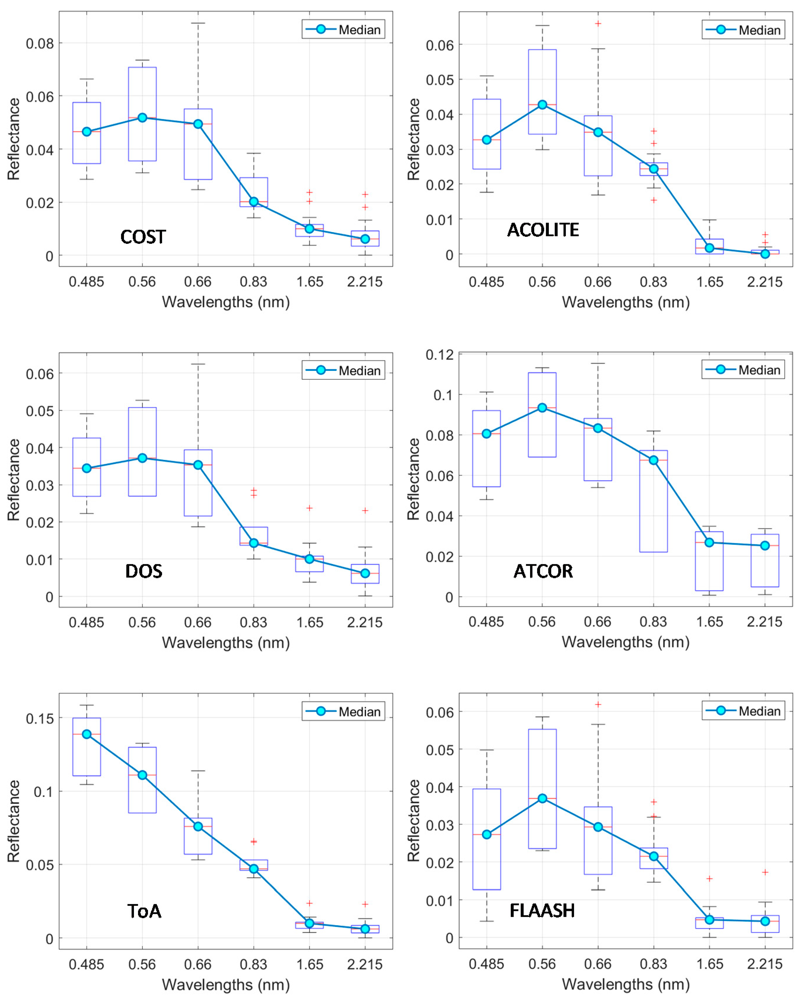
3.1. Spectral Analysis

Figure 4 shows boxplots of the spectral reflectance picked up over the in situ measurements for all models used, including their corresponding medians. Based on the median results, the spectra extracted from the FLAASH, ATCOR, and ACOLITE models have the same shape, typical of case-2 waters; a reflectance peak at the green wavelength, and almost total absorption of backscattered water in longer wavelengths, especially in the SWIR portions. This typical spectral behavior was also perceived for DOS and COST, with a less pronounced reflectance peak at the green. For ToA, no concrete atmospheric correction was made, it was just a conversion of radiance to the reflectance. Hence, shorter wavelengths are most affected by the Rayleigh scattering and consequently, the reflectance at shorter wavelengths is the higher. In fact, by using the dark object subtraction method (for the DOS and COST), it is possible to reduce the additive effect, but the signal recorded by images is still affected by the multiplicative effect. Thereby, the signal is partially corrected using the image-based models, particularly in the visible part of the spectrum, from where the lack of this pronounced peak at the green part of the spectrum originates.

The boxplots show that the boxplot standard deviation (BSD) of reflectance values for all models tended to be narrower above the 830 nm wavelength, except for ATCOR; for which BSDs were large for all bands. It can also be observed that the reflectance’s BSD for the DOS, COST, and ACOLITE models were narrower for the blue band compared to the rest of the models. The boxplots presented here underline the homogeneity of the calibration database reflectance values, except for the NIR and SWIR bands, where some outliers are noticed. This is likely related to the effect of another optically active element, such as the chl_a of algae, which are known to be highly reflective in these spectral regions.

Clearly, the computed reflectance is different from one atmospheric model to another, as was expected. Indeed, modeling is an approximation of reality, and each model is based on its own assumptions to approximate this reality. Notably, the reflectance estimated by the six models converges on the same results, but a slight variability is perceived. This inter-variability (medians) and intra-variability (boxplots) could considerably influence the relationship between spectral indices and in situ SPM concentrations and, consequently, the accuracy of SPM modeling using remote sensing data.

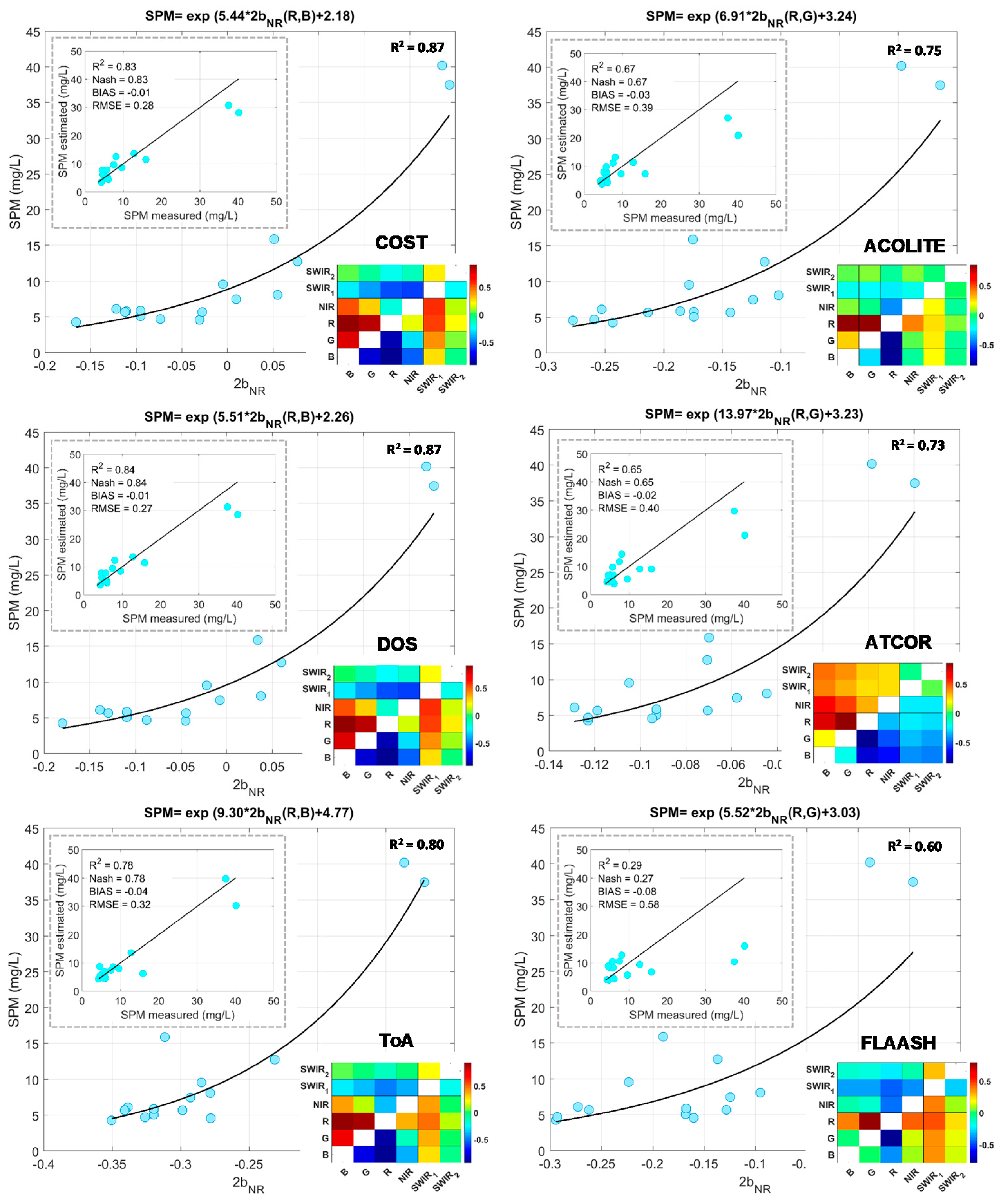
3.2. Modeling of Suspended Particulate Matter

Two main steps were used to model the SPM concentration: (1) calibration of empirical models using a stepwise multivariate regression, and (2) performance evaluation using the cross-validation technique. The evaluation of each model’s performance was quantified using Equations (1)–(4).

3.2.1. Calibration of the Models

It is important to underline that the correlation coefficients from either side of the CCM diagonal are mirrors (see the algorithm on Figure 3). The analysis of the CCMs (presented at the bottom right of Figure 5’s plots) highlights three main findings. First, the correlations of image-based algorithms are practically the same and are very different from those of the physical algorithms. Thus, the SPM relationships to reflectance along the electromagnetic spectrum are controlled by different patterns, depending on the type (image-based or physical) of atmospheric correction model used. Second, the best correlations for image-based algorithms were recorded in the visible part of the spectrum, whereas for physical algorithms the highest correlations were mainly located in the green/red part. Third, correlations of SPM concentrations in the NIR and SWIR parts of the spectrum were qualified as low to modest for most atmospheric correction models. Some relatively moderate correlations (either positive or negative) were, however, recorded for the ATCOR model.

The findings of the CCMs were confirmed with the regression plots. The best stepwise estimator of SPM concentrations was the $2b_{NR}\left(R,B\right)$ (2-band normalized ratio between red and blue bands) for image-based models, whereas the best stepwise estimator of SPM concentrations was the $2b_{NR}\left(R,G\right)$ (green and blue bands) for physical models. In the case of the DOS and COST models, the calibration dot distribution and R² were very similar (the plots are practically the same, but the intercepts and slopes of their calibration functions are slightly different). These findings were expected, because image-based models use a similar algorithm, with only a few differences in the input parameters. Image-based models can explain up to 87% of the SPM concentration variance (R² = 0.87 for the COST and DOS). Physical models were able to explain up to 75% (R² = 0.75 for ACOLITE) of the variance using the same database. It is also important to highlight that all models are univariable, despite some existing high correlations (see CCMs), notably for the ATCOR model.

3.2.2. Cross-Validation of the SPM Modeling

Results of the cross-validation and the statistical evaluation indices are presented in Figure 5 as well (frames at the top left of Figure 5’s plots). Again, image-based models reached the best results, notably for the COST and DOS models. They were almost unbiased and could explain up to 84% of the SPM concentration variance. The robustness of SPM concentration modeling was also confirmed by Nash (up to 0.84). This index is very sensitive, because it uses the mean value of in situ measurements in its evaluation. The slightest estimation error can diminish the Nash results. It is, however, important to emphasize that according to the 1:1 line, except for ToA, all models tend to underestimate high SPM concentrations, with different variability levels. For the physical models, the ACOLITE achieved the best performance, as expected, with R² = Nash = 0.67. The worst results were recorded for the FLAASH model. Again, except for the FLAASH model, all models showed a low bias (<0.04 mg/L), with the best performances recorded equally for the DOS and COST models (=−0.01 mg/L). The models’ RMSE, which quantifies the modeling accuracy, was less than 0.58 mg/L. The best performance was recorded for DOS with 0.27 mg/L, and for the physical models, ACOLITE had the best performance, with an accuracy of 0.39 mg/L.

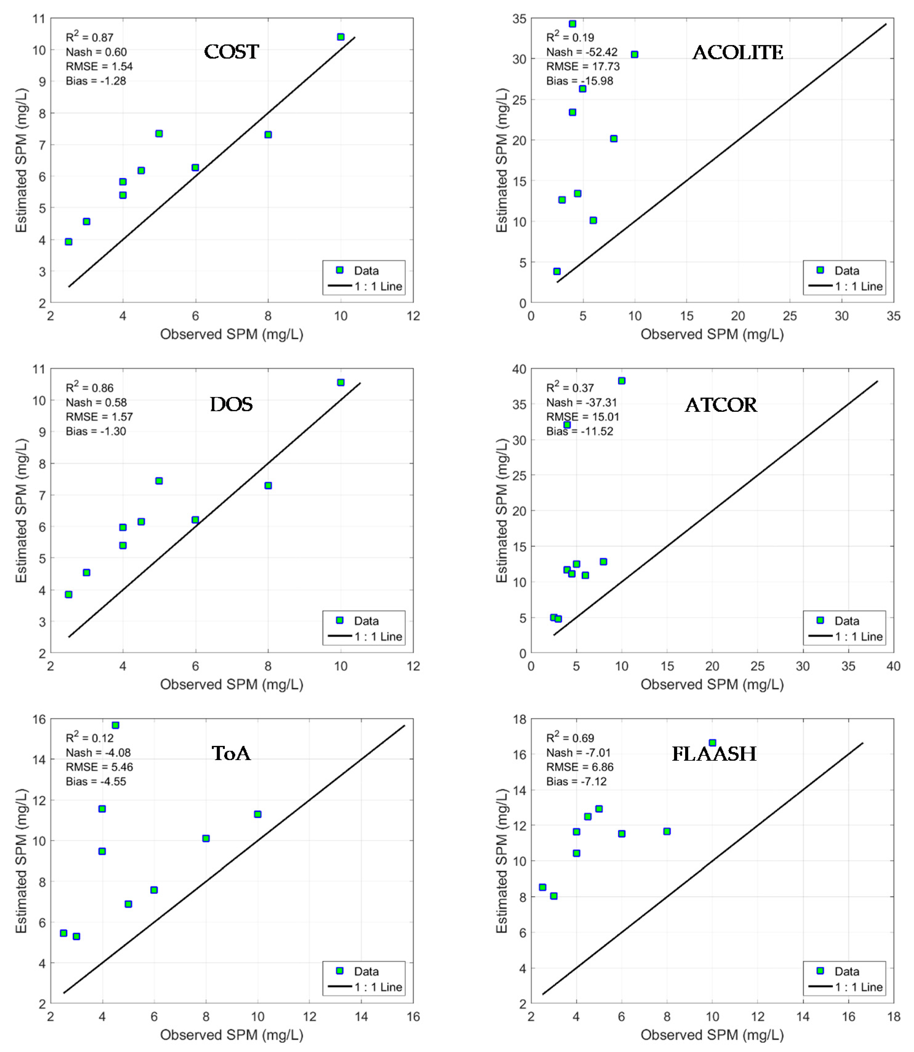
3.2.3. Evaluation of the SPM Modeling with the Blind Test Validation Data

To assess the long-term modeling accuracy, the annual medians of atmospheric correction model Landsat-derived SPM estimates were challenged with in situ SPM measurements (annual medians) collected by the COGESAF monitoring program. The results are presented in Figure 6 and which again underline the high performance of image-based algorithms compared to physical models. The DOS and COST models achieved the best estimates with R² of 0.87 and 0.86 (in the same accuracy range as for the calibration/cross-validation steps) and Nash of 0.60 and 0.58, respectively, highlighting their robustness for long-term modeling. The ToA model did not achieve the same quality of estimates in this validation step. In fact, since the ToA is a radiance to reflectance conversion algorithm, the effect of the atmosphere is not corrected at all (images from one date to another are not “standardized”), which could affect the quality of the SPM modeling. The high performance of ToA in the calibration/cross-validation steps was probably related to the small number (2) of images used and the short date difference between them (August to September). These two months are part of the same season and, therefore, the weather conditions are almost identical. For the validation with the test database, the images used were part of three different seasons (late spring, summer, and early fall). This variation in weather conditions likely played a key role in decreasing the accuracy of the SPM estimates using the same calibration function.

Concerning the physical models, the modeling accuracy was mediocre for all models (Nash <0; this means that the average of the in situ measured SPM data is a better estimator than the model estimates). It is important to recall, however, that the modeling process is generally tainted by two uncertainties: systematic (bias) and random (RMSE) errors. The first is quantifiable and correctable, while the second is not. With this in mind, the FLAASH model could be a potential candidate for the SPM modeling of inland water bodies. Indeed, it is clear that all SPM concentrations are systematically overestimated (the alignment of the points is parallel to the 1:1 line) with an R² of 0.69. Thereby, it would be possible (in future works) to use the bias of this study to systematically correct the SPM concentrations as so: $\widehat{SPM}=\widehat{SPM}+bias.$ This could hugely enhance the modeling accuracy using the FLAASH algorithm.

The results of the blind validation may appear inconsistent, as the accuracy of the FLAASH modeling was the worst for the calibration/cross-validation steps. However, it is important to note the difference, in terms of concentration range, between the two in situ SPM databases (up to 40 mg/L for the calibration/cross-validation database versus up to 10 mg/L for the blind test validation database) that may have played an important role in this incompatibility. According to Figure 5 the FLAASH model tends to significantly underestimate the concentration for high values. In contrast, low SPM values (<10 mg/L) were well distributed around the 1:1 line. Since the blind test validation data does not include high values, this may explain the relatively high performance of the FLAASH model compared to the ACOLITE and ATCOR models for this specific validation database. Therefore, it is necessary to challenge the FLAASH model with higher SPM values.

The above results answered the main hypothesis of this work. Are physical atmospheric correction models, with their complex radiative transfer functions, more appropriate for modeling inland water quality parameters (SPM for this specific work), or are image-based models, with their simplistic corrections, the most appropriate? Whether based on cross-validation or validation with the blind test data, image-based models (DOS and COST) performed the best. Although these results were not expected, they are actually quite logical. Knowing that the water leaving radiance is initially very low (of the order of a hundredth), any slight over- or under-correction of the initial signal recorded by satellite images would alter the reflectance shape along the spectrum and, consequently, the images post-processing.

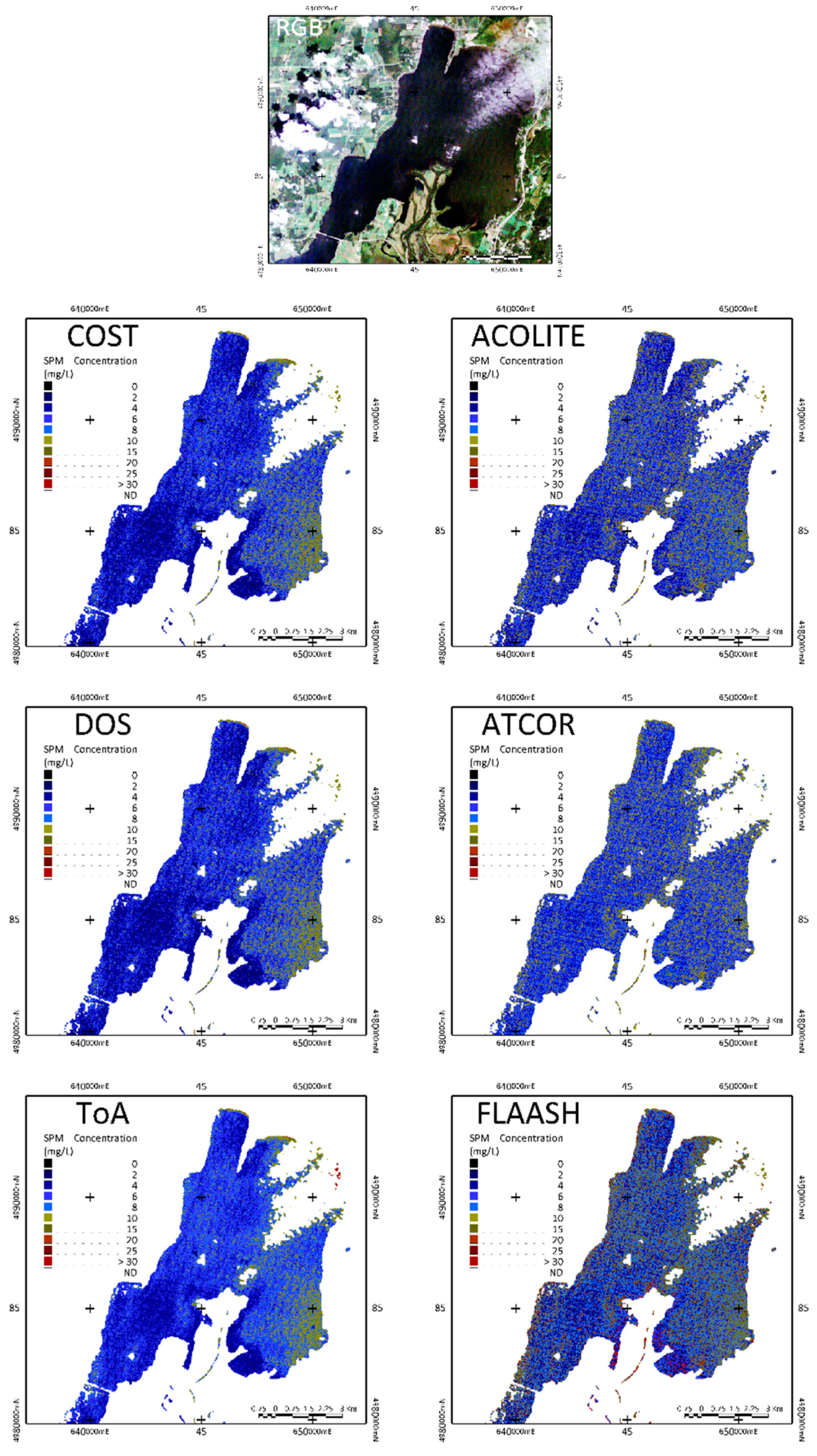
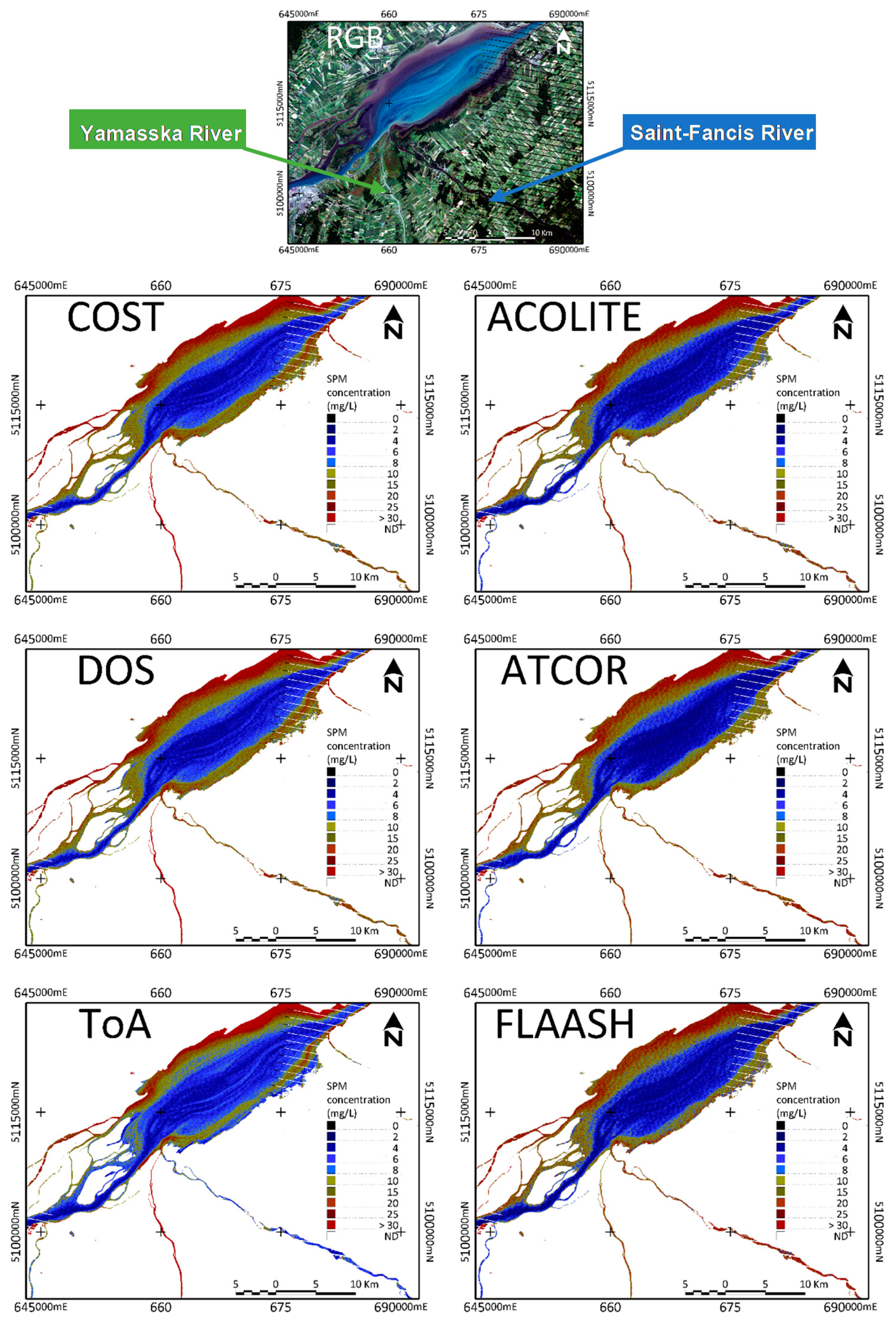
3.2.4. Spatial Distribution Assessment of the SPM

Two images were chosen to compare the atmospheric correction models’ Landsat-derived SPM estimates. These highlight the SPM concentration modeling in two different contexts: waters poor to moderately laden in SPM (in the case of the Missisquoi Bay (M.B.) of Champlain Lake (Figure 7)) and waters highly laden in SPM (in the case of Saint-Pierre (St-P.) Lake (Figure 8)). It is important to highlight that these two images were the ones used in the calibration/cross-validation steps. The SPM maximum in situ concentrations were 12.30 and 40.30 mg/L for M.B. of Champlain Lake and St-P. Lake, respectively (Table 1).

The Figure 7 shows an example of the SPM modeling results over the M.B. of Champlain Lake. From the RGB product, it is clear that the waters are poor to moderately laden with SPM (dark shade), which is also confirmed by the outputs of all models. However, image-based models seem to better reproduce the spatial distribution, as it is perceived on the RGB product, compared to physical models. For the latter, the SPM spatial distribution is lost and the estimate seems to be random (pixels with high to very high concentrations are adjacent to pixels with low to very low concentrations, giving a salt and pepper aspect to SPM the modeling).

On the other hand, when waters were highly laden with SPM, the spatial distribution was quite similar for all the model outputs (Figure 8). It is, however, important to underscore that SPM concentrations were slightly overestimated by all the models compared to the outputs of the ToA-based model, particularly for the St-F. (Saint Francis) river. According to [35,36], the St-F. River is known to drain waters with low to moderate SPM concentrations and the Yamaska river (Y.R.) is known to drain waters with the highest SPM concentrations in the St. Lawrence basin [37]. This is because the two tributaries belong to different watersheds. The St-F. River watershed is composed of 66% forested lands (versus 42% for the Y. R.) and of 23% agrarian lands (versus 54% for the Y. R.) [38]. This may explain this remarkable difference in the SPM load of the two rivers. In all model outputs, the Y.R. is associated with high SPM concentrations, confirming the assumption that all models reach the same accuracy when waters are highly laden in SPM. On the other hand, excepting the image-based models, the physical models also associated high to very high SPM concentrations with the St-F. River. This was expected, as all physical models tend to overestimate low to medium SPM concentrations (Figure 6).

4. Discussions

The above results illustrate the ability of remote sensing data to estimate the SPM concentrations in inland water bodies with an acceptable accuracy rate, when using the right atmospheric correction model. Contrary to expectations, the results highlighted that image-based atmospheric models are the best for retrieving SPM concentrations. This finding is nonetheless coherent with the results of Nazeer, Nichol [39], who assessed five different atmospheric correction methods, including three physical methods (6S, FLAASH, and ATCOR) and two image-based methods (DOS and ELM) using in situ multispectral radiometer measurements (as a radiometric analysis, unlike this study which used a limnological-based analysis). They concluded that the DOS method outperformed the FLAASH and ATCOR methods.

In addition, our results highlighted a strong correlation with $2b_{NR}\left(R,B\right)$ when using image-based images, versus $2b_{NR}\left(R,G\right)$ when using physical images. This may be related to the fact that physical algorithms tend to over-correct the reflectance in the blue part of the spectrum compared to the image-based models (Figure 4). Indeed, the short wavelengths of the spectrum (some parts of ultraviolet and most of the blue) are less absorbed by clear waters and consequently penetrate the deepest in the water column [19]. Thus, there is an inverse correlation between the reflectance captured by the blue band and the concentration of SPM (the less SPM, the clearer the water [3]). This relationship is most likely due to the strong absorption of CDOM or chl_a from algae in this part of the spectrum. On the other hand, the presence of SPM in water causes turbidity. Turbid waters (caused either by SPM [40], dissolved organic carbon [41], algal blooms [40], etc.) are known to reflect strongly in the red part of the spectrum. Therefore, this natural optical contrast (strong absorption in the blue versus strong reflection in the red) across the spectrum, should be most correlated with SPM. The overcorrection of the blue band reflectance by physical models probably destroys this natural physical dependence that exists between the SPM concentration and the energy absorbed by waters in the blue part of the spectrum and shifts it to the closest band (green; less correlated with clear waters). This may explain the higher correlations for image-based algorithms (up to 87%), which are based on the blue Landsat band, and the relatively lower correlations (up to 75%) for physical models, which are based on the green Landsat band (Figure 5).

Physical atmospheric correction methods usually use two or more NIR (or SWIR) wavebands, where the marine signal is assumed to be zero (open ocean waters), thus the signal in the NIR (or SWIR) can be regarded as entirely atmospheric, and it is used to determine the aerosol model. However, the signal in the NIR (or SWIR) is not negligible in case-2 waters, due to the concentrations of particulate matter in inland water bodies, and, consequently, maritime correction over inland water causes low or even negative water reflectance in the visible bands [15,16,42]. In addition, the physical models’ inputs are not initially optimized to generate accurate reflectance estimates for inland water bodies. Indeed, limited choices of aerosol type are available in commercial remote sensing software; for instance, rural, desert, urban, and maritime are the choices available for the ATCOR plug-in integrated into PCI Geomatics. The nearest choice would be the rural option, but it is not optimal for inland waters, since the aerosols captured by these aquatic systems are very different from those located on top of forests or on crops in agricultural fields. The rural option is optimized to correct the aerosols of vegetation more than those of water bodies [39]. As a consequence, reflectance over inland water bodies is estimated based on incorrect assumptions (0 water-leaving radiance in the NIR (or SWIR) and aerosol origin/type models), leading to the destruction of this natural optical–physical relationship (in terms of reflectance) of the water parameters across the electromagnetic spectrum.

5. Conclusions

The goal of this work was to compare the performance image-based atmospheric correction (ToA, DOS, and COST) models to the common physical models (ATCOR, FLAASH, and ACOLITE) most used for retrieving SPM concentrations in inland water bodies. Landsat images were used for this purpose. The results highlighted the potential of remote sensing data to retrieve SPM concentrations. The best performances were recorded for the image-based models (R² up to 0.84, Nash up to 0.84, bias down to −0.01 mg/L, RMSE down to 0.27 mg/L) using the blue-red spectral indices. The results of physical models were acceptable (R² up to 0.67, Nash up to 0.67, bias down to −0.02 mg/L, RMSE down to 0.39 mg/L) using the green-red spectral indices. Validation with the blind test data, as a long-term analysis, also affirmed the above finding, with an R² up to 0.87, Nash up to 0.60, bias down to −1.28 mg/L, and RMSE down to 1.54 mg/L. Nevertheless, the accuracy of the ToA decreased significantly, probably due to large weather variations resulting from the long-term analysis. The spatial distribution of SPM concentration estimates underlined the good performance of image-based models when waters are poorly to moderately laden with SPM. For water highly laden with SPM, the modeling accuracy was almost the same for all models. To summarize, the results of this study highlighted that image-based models, particularly the COST and DOS, are more appropriate than physical models for retrieving SPM concentrations in inland waters if the inputs of the physical atmospheric parameters are not well controlled. Reanalysis of these results using a larger database and covering a wider range of SPM concentrations is strongly recommended and would help to approve/disapprove our results. Nevertheless, challenges are still on the table to remotely estimate inland water quality parameters using satellite images for large-scale applications. To this end, the development of physical atmospheric correction algorithms specific to inland waters is greatly needed.

References

1. Håkanson, L.; Eckhéll, J. Suspended particulate matter (SPM) in the Baltic Sea—New empirical data and models. Ecol. Model. 2005, 189, 130–150. [Google Scholar] [CrossRef]
2. Liu, D.; Duan, H.; Yu, S.; Shen, M.; Xue, K. Human-induced eutrophication dominates the bio-optical compositions of suspended particles in shallow lakes: Implications for remote sensing. Sci. Total. Environ. 2019, 667, 112–123. [Google Scholar] [CrossRef] [PubMed]
3. Houma, F.B. Modélisation et Cartographie de la Pollution Marine et de La Bathymétrie à Partir de L’imagerie Satellitaire. Ph.D. Thesis, Université Paris-Est, Créteil, France, 2009. [Google Scholar]
4. Liu, H.; Li, Q.; Shi, T.; Hu, S.; Wu, G.; Zhou, Q. Application of Sentinel 2 MSI Images to Retrieve Suspended Particulate Matter Concentrations in Poyang Lake. Remote Sens. 2017, 9, 761. [Google Scholar] [CrossRef] [Green Version]
5. Robert, E.; Kergoat, L.; Soumaguel, N.; Merlet, S.; Martinez, J.-M.; Diawara, M.; Grippa, M. Analysis of Suspended Particulate Matter and Its Drivers in Sahelian Ponds and Lakes by Remote Sensing (Landsat and MODIS): Gourma Region, Mali. Remote Sens. 2017, 9, 1272. [Google Scholar] [CrossRef] [Green Version]
6. Giani, A.; Bird, D.F.; Prairie, Y.; Lawrence, J.F. Empirical study of cyanobacterial toxicity along a trophic gradient of lakes. Can. J. Fish. Aquat. Sci. 2005, 62, 2100–2109. [Google Scholar] [CrossRef]
7. Carmichael, W.W. An Overview of Toxic Cyanobacteria Research in the United States: Toxic Cyanobacteria: Current Status of Research and Management; Australian Centre for Water Quality Research: Salisbury, Australia, 1994. [Google Scholar]
8. Chorus, I.; Bartram, J. Toxic Cyanobacteria in Water. A Guide to Their Public Health Consequences, Monitoring and Management; E & FN Spon, for World Health Organization, Routledge: London, UK, 1999; p. 416. [Google Scholar]
9. Svrcek, C.; Smith, D.W. Cyanobacteria toxins and the current state of knowledge on water treatment options: A review. J. Environ. Eng. Sci. 2004, 3, 155–185. [Google Scholar] [CrossRef]
10. Chen, J.; Quan, W.; Cui, T.; Song, Q. Estimation of total suspended matter concentration from MODIS data using a neural network model in the China eastern coastal zone. Estuar. Coast. Shelf Sci. 2015, 155, 104–113. [Google Scholar] [CrossRef]
11. Doxaran, D.; Froidefond, J.-M.; Lavender, S.; Castaing, P. Spectral signature of highly turbid waters: Application with SPOT data to quantify suspended particulate matter concentrations. Remote Sens. Environ. 2002, 81, 149–161. [Google Scholar] [CrossRef]
12. Topliss, B.; Almos, C.; Hill, P. Algorithms for remote sensing of high concentration, inorganic suspended sediment. Int. J. Remote Sens. 1990, 11, 947–966. [Google Scholar] [CrossRef]
13. Zhang, M.; Dong, Q.; Cui, T.; Xue, C.; Zhang, S. Suspended sediment monitoring and assessment for Yellow River estuary from Landsat TM and ETM+ imagery. Remote Sens. Environ. 2014, 146, 136–147. [Google Scholar] [CrossRef]
14. Moore, G.F.; Aiken, J.; Lavender, S.J. The atmospheric correction of water colour and the quantitative retrieval of suspended particulate matter in Case II waters: Application to MERIS. Int. J. Remote Sens. 1999, 20, 1713–1733. [Google Scholar] [CrossRef]
15. Ruddick, K.G.; Ovidio, F.; Rijkeboer, M. Atmospheric correction of SeaWiFS imagery for turbid coastal and inland waters. Appl. Opt. 2000, 39, 897–912. [Google Scholar] [CrossRef] [Green Version]
16. Shang, P.; Shen, F. Atmospheric Correction of Satellite GF-1/WFV Imagery and Quantitative Estimation of Suspended Particulate Matter in the Yangtze Estuary. Sensors 2016, 16, 1997. [Google Scholar] [CrossRef] [Green Version]
17. Wang, C.; Chen, S.; Li, D.; Wang, D.; Liu, W.; Yang, J. A Landsat-based model for retrieving total suspended solids concentration of estuaries and coasts in China. Geosci. Model Dev. 2017, 10, 4347–4365. [Google Scholar] [CrossRef] [Green Version]
18. Pahlevan, N.; Lee, Z.; Wei, J.; Schaaf, C.; Schott, J.R.; Berk, A. On-orbit radiometric characterization of OLI (Landsat-8) for applications in aquatic remote sensing. Remote Sens. Environ. 2014, 154, 272–284. [Google Scholar] [CrossRef]
19. Gholizadeh, M.H.; Melesse, A.M.; Reddi, L. A Comprehensive Review on Water Quality Parameters Estimation Using Remote Sensing Techniques. Sensors 2016, 16, 1298. [Google Scholar] [CrossRef] [PubMed] [Green Version]
20. Mishra, S.; Mishra, D.; Schluchter, W.M. A Novel Algorithm for Predicting Phycocyanin Concentrations in Cyanobacteria: A Proximal Hyperspectral Remote Sensing Approach. Remote Sens. 2009, 1, 758–775. [Google Scholar] [CrossRef] [Green Version]
21. Rahman, H. Influence of atmospheric correction on the estimation of biophysical parameters of crop canopy using satellite remote sensing. Int. J. Remote Sens. 2001, 22, 1245–1268. [Google Scholar] [CrossRef]
22. Curcio, J. Evaluation of Atmospheric Aerosol Particle Size Distribution from Scattering Measurements in the Visible and Infrared. J. Opt. Soc. Am. 1961, 51, 548–551. [Google Scholar] [CrossRef]
23. Sabins, F.F., Jr. Remote Sensing-Principles and Interpretation; WH Freeman and Company: New York, NY, USA, 1987. [Google Scholar]
24. Turner, R.; Malila, W.; Nalepka, R. Importance of atmospheric scattering in remote sensing, or everything you’ve always wanted to know about atmospheric scattering but were afraid to ask. In Proceedings of the International Symposium on Remote Sensing of Environment, Ann Arbor, MI, USA, 17–21 May 1971. [Google Scholar]
25. Morel, A.; Bélanger, S. Improved detection of turbid waters from ocean color sensors information. Remote Sens. Environ. 2006, 102, 237–249. [Google Scholar] [CrossRef]
26. Lavender, S.; Pinkerton, M.; Moore, G.; Aiken, J.; Blondeau-Patissier, D. Modification to the atmospheric correction of SeaWiFS ocean colour images over turbid waters. Cont. Shelf Res. 2005, 25, 539–555. [Google Scholar] [CrossRef]
27. Vanhellemont, Q.; Ruddick, K. Advantages of high quality SWIR bands for ocean colour processing: Examples from Landsat-8. Remote Sens. Environ. 2015, 161, 89–106. [Google Scholar] [CrossRef] [Green Version]
28. Richter, R. Correction of atmospheric and topographic effects for high spatial resolution satellite imagery. Int. J. Remote Sens. 1997, 18, 1099–1111. [Google Scholar] [CrossRef]
29. Richter, R. Atmospheric correction of satellite data with haze removal including a haze/clear transition region. Comput. Geosci. 1996, 22, 675–681. [Google Scholar] [CrossRef]
30. Anderson, G.P.; Felde, G.W.; Hoke, M.L.; Ratkowski, A.J.; Cooley, T.W.; Chetwynd, J.J.H.; Gardner, J.A.; Adler-Golden, S.M.; Matthew, M.W.; Berk, A.; et al. MODTRAN4-based atmospheric correction algorithm: FLAASH (Fast Line-of-sight Atmospheric Analysis of Spectral Hypercubes). In Algorithms and Technologies for Multispectral, Hyperspectral, and Ultraspectral Imagery VIII; International Society for Optics and Photonics: Bellingham, WA, USA, 2002. [Google Scholar]
31. Kotchenova, S.Y.; Vermote, E.F.; Matarrese, R.; Klemm, J.F.J. Validation of a vector version of the 6S radiative transfer code for atmospheric correction of satellite data Part I: Path radiance. Appl. Opt. 2006, 45, 6762–6774. [Google Scholar] [CrossRef] [PubMed] [Green Version]
32. Moran, M.; Jackson, R.D.; Slater, P.N.; Teillet, P.M. Evaluation of simplified procedures for retrieval of land surface reflectance factors from satellite sensor output. Remote Sens. Environ. 1992, 41, 169–184. [Google Scholar] [CrossRef]
33. Chavez, P.S., Jr. An Improved Dark-Object Subtraction Technique for Atmospheric Scattering Correction of Multispectral data. Remote Sens. Environ. 1988, 24, 459–479. [Google Scholar] [CrossRef]
34. Chavez, P.S. Image-based atmospheric corrections-revisited and improved. Photogramm. Eng. Remote Sens. 1996, 62, 1025–1035. [Google Scholar]
35. Laliberté, D. La Qualité de L’eau des Rivières Richelieu et Yamaska; Ministère de L’Environnement et de la Lutte contre les Changements Climatiques, Ed.; Gouvernement du Québec: Montréal, QC, Canada, 2015. [Google Scholar]
36. OBVY. Diagnostic du Bassin Versant de la Rivière Yamaska; OBVY, Ed.; Regroupement des Organismes de Bassins Verssants du Québec: Québec, QC, Canada, 2009. [Google Scholar]
37. COGESAF. Outil de Cartographie Dynamique du Conseil de Gouvernance de L’eau des Bassins Versants de la Rivière Saint-François. 2003–2018. Available online: http://cogesaf.sigmont.org/cogesaf/cogesaf.php (accessed on 28 January 2020).
38. Caron, S.; Lucotte, M.; Teisserenc, R. Mercury transfer from watersheds to aquatic environments following the erosion of agrarian soils: A molecular biomarker approach. Can. J. Soil Sci. 2008, 88, 801–811. [Google Scholar] [CrossRef] [Green Version]
39. Nazeer, M.; Nichol, J.E.; Yung, Y.-K. Evaluation of atmospheric correction models and Landsat surface reflectance product in an urban coastal environment. Int. J. Remote Sens. 2014, 35, 6271–6291. [Google Scholar] [CrossRef]
40. Kahru, M.; Mitchell, B.G.; Diaz, A.; Miura, M. MODIS detects a devastating algal bloom in Paracas Bay, Peru. Eos 2004, 85, 465–472. [Google Scholar] [CrossRef] [Green Version]
41. Toming, K.; Kutser, T.; Laas, A.; Sepp, M.; Paavel, B.; Nõges, T. First Experiences in Mapping Lake Water Quality Parameters with Sentinel-2 MSI Imagery. Remote Sens. 2016, 8, 640. [Google Scholar] [CrossRef] [Green Version]
42. Gordon, H.R.; Wang, M. Retrieval of water-leaving radiance and aerosol optical thickness over the oceans with SeaWiFS: A preliminary algorithm. Appl. Opt. 1994, 33, 443–452. [Google Scholar] [CrossRef] [PubMed]
Figure 1. Geographic location of in situ samples; red frame (Missisquoi Bay (M.B.) of Lake Champlain) and blue frame (Lake St. Pierre (St-P.)) used for calibration and cross-validation, and green frame (St. Francis River) used for testing.
Water 13 02149 g001
Figure 2. Flowchart of the methodological approach; blue frames refers to calibration and cross-validation steps, and orange frames refer to the testing step.
Water 13 02149 g002
Figure 3. The correlation coefficient matrix algorithm (A) with its outputs (B).
Water 13 02149 g003
Figure 4. Boxplots of reflectance spectra of the calibration database processed by the six atmospheric models and their corresponding median.
Water 13 02149 g004
Figure 5. The 2-band normalized ratio ( 2 b N R ) values versus concentration of suspended particulate matters (SPM) for different atmospheric correction algorithms for Landsat data with their corresponding correlation coefficient matrices (CCMs). Integrated plots show the cross-validation results with the corresponding statistical evaluation indices.
Water 13 02149 g005
Figure 6. Modeling assessment with the blind test validation database.
Water 13 02149 g006
Figure 7. Landsat true color image of the Missisquoi Bay of Champlain Lake (25 August 2009) and the derived SPM concentrations by the different atmospheric correction models.
Water 13 02149 g007
Figure 8. Landsat true color of Lake Saint-Pierre (2 September 2009) and the SPM concentration derived by the different atmospheric correction models.
Water 13 02149 g008