Development of a Practical Model for Predicting Soil Salinity in a Salt Marsh in the Arakawa River Estuary

Abstract

Our group has studied the spatiotemporal variation of soil and water salinity in an artificial salt marsh along the Arakawa River estuary and developed a practical model for predicting soil salinity. The salinity of the salt marsh and the water level of a nearby channel were measured once a month for 13 consecutive months. The vertical profile of the soil salinity in the salt marsh was measured once monthly over the same period. A numerical flow simulation adopting the shallow water model faithfully reproduced the salinity variation in the salt marsh. Further, we developed a soil salinity model to estimate the soil salinity in a salt marsh in Arakawa River. The vertical distribution of the soil salinity in the salt marsh was uniform and changed at almost the same time. The hydraulic conductivity of the soil, moreover, was high. The uniform distribution of salinity and high hydraulic conductivity could be explained by the vertical and horizontal transport of salinity through channels burrowed in the soil by organisms. By combining the shallow water model and the soil salinity model, the soil salinity of the salt marsh was well reproduced. The above results suggest that a stable brackish ecotone can be created in an artificial salt marsh using our numerical model as a design tool.

1. Introduction

The flood plains along rivers are often expected to function as natural reserves in highly populated metropolitan areas of Japan such as Tokyo and Osaka, where the residents have very few opportunities to encounter Nature near their homes [1]. Yet if the river in a metropolitan area is small, such as the Sumida River in Tokyo [2] or the Seine River in Paris, the upright revetments of concrete along the riverbank are not conducive to the creation of a Nature-oriented river environment. On the other hand, large-sized rivers in Japan have wide riverbanks [3] that permit the creation of various habitat zones along the riverbank [1]. In a tidal section in particular, the run-up of saltwater with tidal fluctuations changes the water level, enabling the creation of a salt marsh. When a riverbank is composed of marshland, the inflow and outflow of salt water as the water level falls and rises forms a salt marsh, and salt water enters and exits between the inundated water and soil composing the marsh [4,5]. This saline condition effects brackish fish and benthic organisms [6,7]. The salinity of not only water, but also of soil, is thought to be an important determinant of the habitability of an environment for benthic organisms like crabs, worms, etc. [5,8,9,10,11]. The relationship between the salinity in a channel, a source of salinity, and that in a marsh, must therefore be considered when creating a salt marsh artificially. There is no example of the artificial development of such a salt marsh, largely because of the difficulties in controlling the salinity conditions. While a brackish water condition is maintained in a small-scale artificial marsh (such a riverine marsh or lagoon is called a “wand” in Japanese, such as the “Gotanno-wand”) in the downstream section of Arakawa River in downtown Tokyo, that condition was not intended at the time of the marsh’s construction design.

As a basic step to research the possibility of creating a salt marsh on the banks of a channel, we observed time-series changes of salinity in the marsh caused by tidal action. We then developed a model that faithfully reproduced the observed data by combining a plane two-dimensional flow model with the salt transport equation. After the marsh was flooded with fresh water in the typhoon at October 2019, we observed the soil salinity about once a month to examine the salinity recovery process. Finally, we developed a series of numerical models to predict the soil salinity in the marsh.

2. Materials and Methods

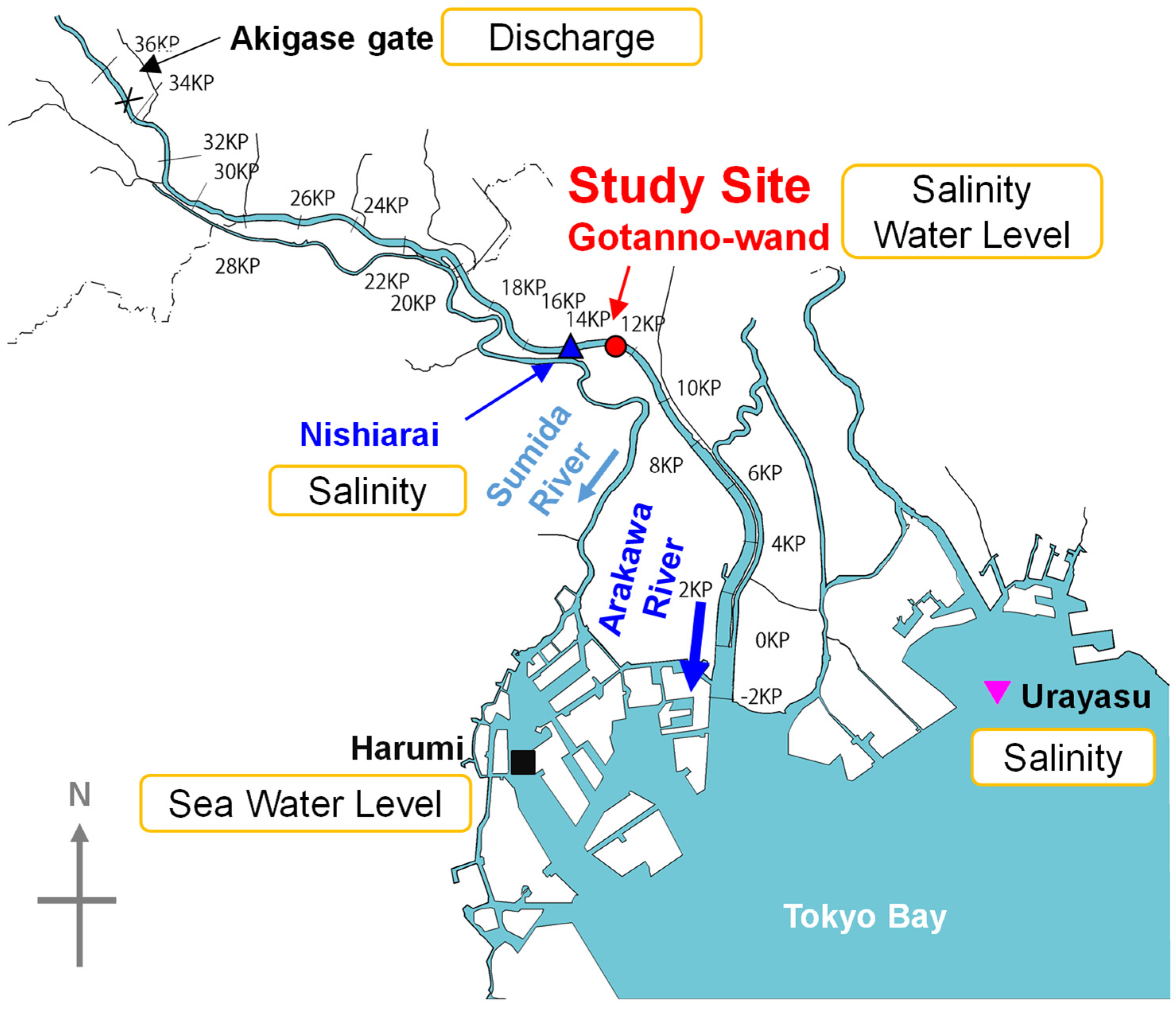
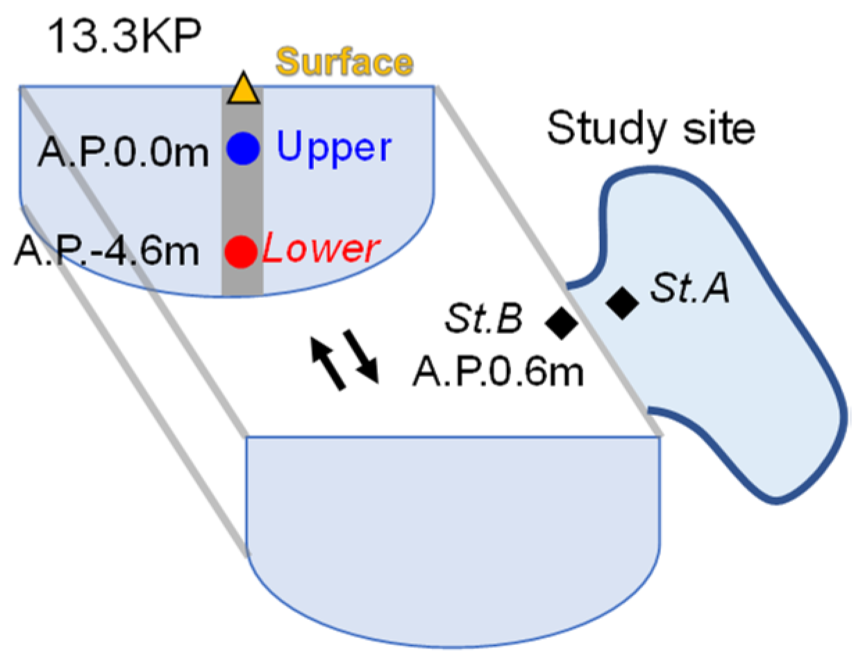
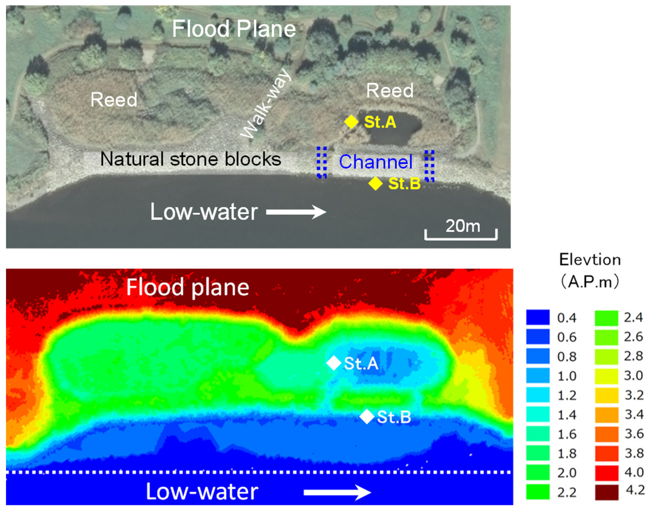
2.1. Study Site

Figure 1 shows the research study area in Arakawa, a large river that flows through Saitama Prefecture and Tokyo Metropolis, with a tidal section downstream from the Akigase Weir (35 km). The Gotanno-wand, the subject of this study, covers an area of about 0.7 ha near Arakawa (12 km) (●). The observation data at each point are shown in Figure 1. The salinity of Nishiarai Observatory (12 km) is observed in the upper and lower layers, as shown in Figure 2.

During non-flood conditions in the channel, the water level fluctuates by around 2 m according to the tidal level in Tokyo Bay. The tide, therefore, is considered the main determinant of the flow during normal-water conditions. The riverine marsh studied is located on the left-hand bank, about 12 km from the river mouth, as shown in Figure 1. The width and the depth of the river channel at this section are about 400 m and 6 m, respectively. The river water is mildly stratified on neap-tide days and is well mixed vertically on spring-tide days. Figure 3 shows a plane view and elevation contour of the riverine marsh. A small shallow pond to the right of the walk-way and the surrounding salt marsh are covered by a reed community. The marsh is separated from the river channel by a porous dike made of natural stones of about 50–80 cm in diameter, on which two shallow channels are located to maintain sufficient water exchange between the river channel and marsh. The photographs in Figure 4 show worms and brackish water organisms that form burrows in the ground and usually live in the soil. The photograph on the left shows two crab burrows and a large number of smaller holes left by worms on the surface of the land area (St. A) on neap-tide days.

2.2. Field Measurement

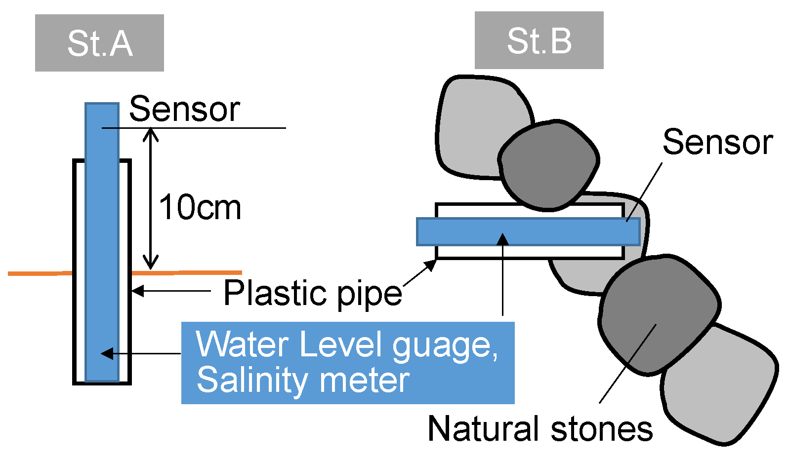
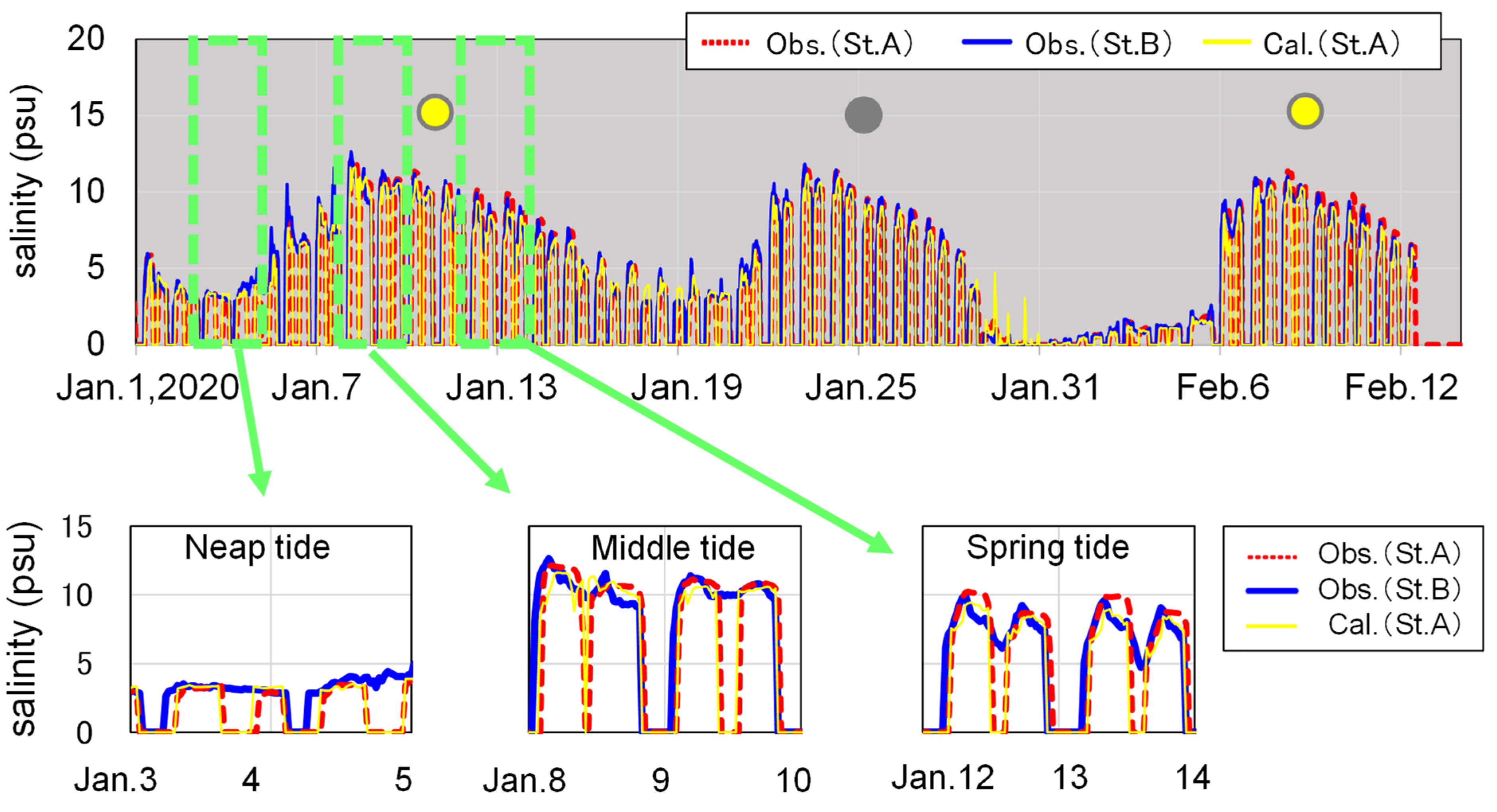
2.2.1. Water Salinity and Water Level

Portable salinity meters (HOBO U24-002-C, Onset, Bourne, MA, USA) and self-recording water level gauges (Onset HOBO U20-001-01-TI) were installed at the two places indicated in Figure 3 (◆). The sensor units of the measurement devices were kept 10 cm higher than the ground at both installation sites to avoid the influence of sediment. All of the sensors were exposed to open air during neap-tide days (Figure 5).

The upper chart of Figure 6 plots the Akigase Weir (35 km) discharge and tidal level recorded at the Harumi Observatory (Tokyo Bay), the middle chart plots the salinity at Urayasu (Tokyo Bay), and the lower chart plots the salinity measured at the Nishiarai Observatory (13 km) and St. B (12 km). The salinity was higher at St. B than in the upper layer measured at the Nishiarai Observatory. From this year-round observation data, we see that the salinity remains significantly lower from late April to early October, compared with the rest of the year. This seasonal drop in salinity is thought to result from the dilution of the salinity of Tokyo Bay by the river water inflow during the flood season.

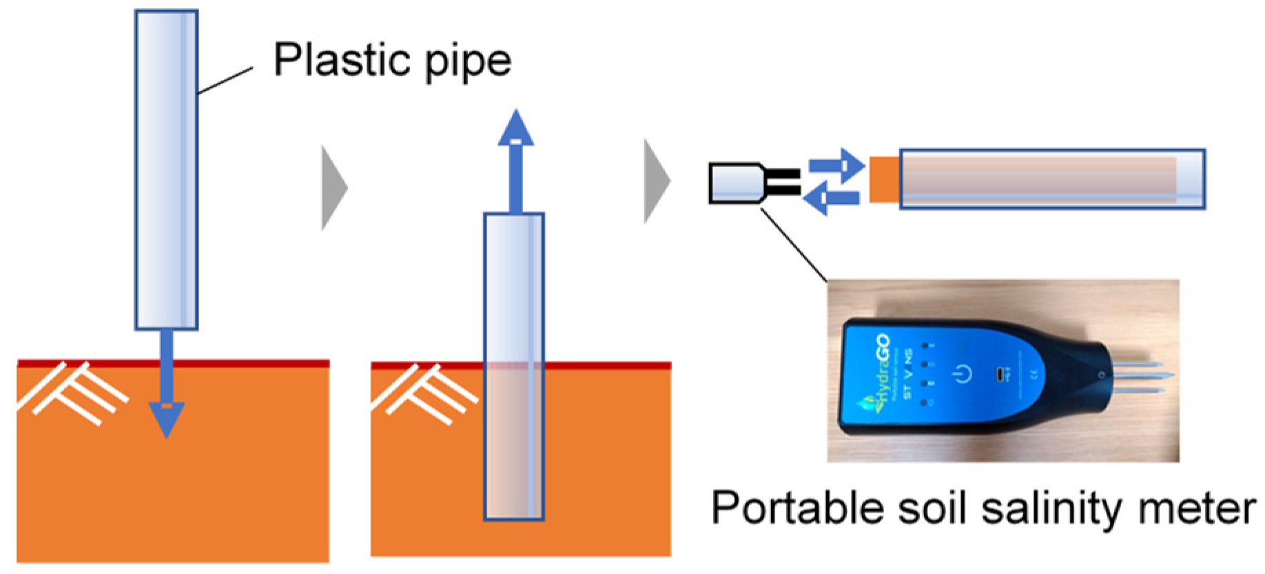
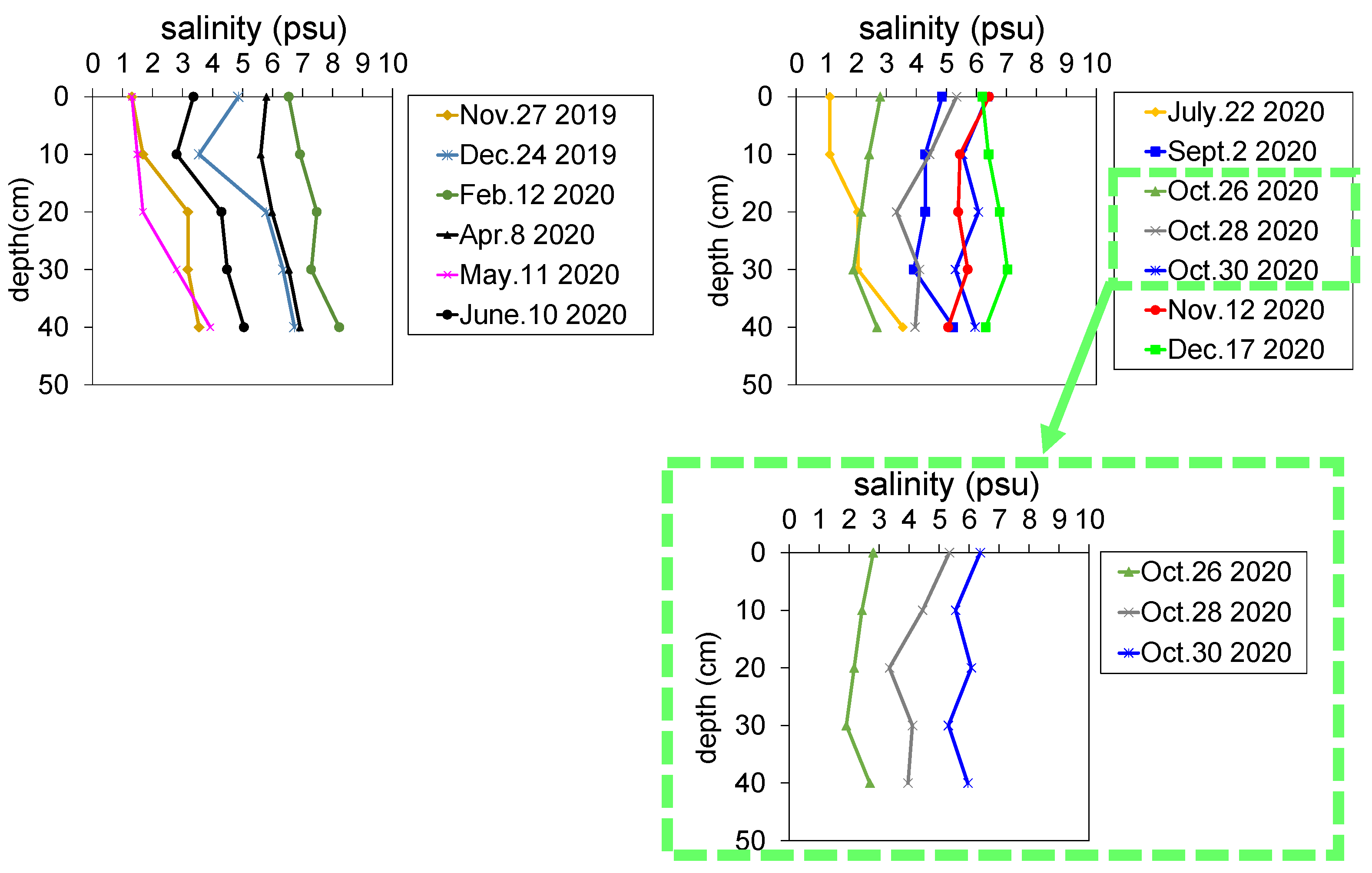
2.2.2. Soil Salinity

Roughly once per month, soil cores of 40 cm in length were sampled vertically at St. A, when the ground surface appeared at ebb tide, and the pore water salinity was measured at successive depth intervals of 10 cm from the ground surface using the portable soil salinity meter shown in Figure 7. The soil salinity measurements were performed in the following steps. A PVC pipe was pushed through the ground surface to a predetermined depth and pulled out, a rod slightly smaller in diameter than the PVC pipe was inserted from the head, and a portable soil multi-probe (HydraGO made of stainless steel with a length of 5.7 cm, STEVENS, Portland, OR, USA) was inserted into several cm of exposed soil sample. Since the output of this device was affected by the size and density of the soil particles [12,13,14,15,16], it was converted to a value of 1:5 according to the water leaching method (Japanese Standards Association, 2020) using a correction curve.

The chart on the upper left of Figure 8 shows the results of on-site measurements of soil salinity taken at St. A from 27 November 2019 to June 2020. The chart on the right shows soil salinity values obtained by subsequent on-site measurement. These soil salinity values fluctuate almost uniformly in all layers, including that at a 40 cm depth from the ground surface. As an additional step to understand the rate of change in soil salinity on a daily basis, we conducted the same survey every two days in October 2020. The results are shown in the bottom of Figure 8. The soil salinity was found to have increased almost uniformly in all layers, and the salinity that flowed into the marsh rapidly infiltrated into the soil.

2.2.3. Hydraulic Conductivity

As shown in the photograph on the left in Figure 4, the many burrows left by crabs and brackish worms are thought to affect the infiltration of salt water into the soil. To understand the vertical distribution of channels left by burrowing organisms, the number of channels in a cross section of a soil sample collected from the surface at St. A at a pitch of 10 cm was confirmed at the site. As a result, 8, 4, 1, and 3 channels were visually confirmed at depths of 10, 20, 30, and 40 cm, respectively.

Based on the above, a hydraulic conductivity test of the soil was conducted in the marsh. Samples were collected without spillage by penetrating PVC pipes through the surface layer (0–8 cm), middle layer (16–24 cm), and lower layer (32–40 cm). The hydraulic conductivity test was performing using the variable water level method [17]. The hydraulic conductivity was calculated by the following equation [17]:

$$k=\frac{L}{\left(t_2-t_1\right)}ln\frac{h_1}{h_2}=\frac{2.303L}{\left(t_2-t_1\right)}{\log }_{10}\frac{h_1}{h_2}$$

(1)

where, k (cm/s) is the hydraulic conductivity, L (cm) is vertical length of soil sample in acrylic pipe (diameter is 6 cm), $t_1$ (s) is the elapsed time at the initial water level (zero), $t_2$ (s) is the elapsed time from the initial water level, $h_1$ (cm) is the initial water level at $t_1$, and $h_2$ (cm) is the water level at $t_2$.

The hydraulic conductivity at each layer was calculated to understand how the hydraulic conductivity differed in accordance with the presence or absence of burrows left by organisms. The hydraulic conductivity k of the undisturbed sample was 1.3 × 10⁻¹, 6.6 × 10⁻², and 1.9 × 10⁻² (cm/s) from the surface layer, respectively. These k values were equivalent to the value of gravel [18]. On the other hand, the hydraulic conductivity k of a sample disturbed by hand was 1.2 × 10⁻⁶ (cm/s). In this hand-disturbed sample, 20% of the particle sizes measured 0.007 mm, a size confirmed to have k value on the order of 1 × 10⁻⁶ (cm/s) [18]. The hydraulic conductivity of the undisturbed sample has found to be 10⁴ orders higher than the value determined by the soil particle size.

2.3. Numerical Model

2.3.1. Water Salinity

A numerical flow model based on shallow water equations, including a salinity balance equation, was used to simulate the water exchange between the river and marsh, as well as the flow within the marsh. The salt advection-diffusion equation was added to the shallow water flow model [19] of a general rectangular lattice to obtain the salinity spatial change. The grid size was defined as 1 m × 1 m, and the topographical data were set. The Manning roughness coefficient of the ground surface was set at 0.08 for the reed area, 0.02 for bare land (outside reed area), and 0.05 for the dike, referring to the 2002 Guide for the Study of River Channel Planning Japan Institute of Construction Engineering [20]. A boundary condition was set in the position marked by the dotted line to the low-water channel in Figure 3. While some inflow and outflow through the gaps of the dike were noted, the amounts were thought to be small enough to disregard in the analysis.

2.3.2. Soli Salinity

The salt exchange rate between surface water and soil pore water is determined by the particle size and openness of the soil, as well as the activities of benthic animals (burrows and passageways left by organisms such as crabs and worms). The rate, however, is difficult to determine by quantitative means. Instead, therefore, we followed the method of Lin et al. [5] using a transfer equation expressed by a first-order differential equation and identifying the empirical constant γ from the observed data:

$$\frac{d}{dt}\left\{S_f\left(t\right)\right\}=\gamma \left\{S_0\left(t\right)-S_f\left(t\right)\right\}$$

(2)

where, $\gamma$ is the empirical water conductivity of the soil layer, $S_0\left(t\right)$ is the salinity of water covering the ground, and $S_f\left(t\right)$ is the vertical average of the soil salinity. It has been confirmed that the salinity of the riverbank and the water salinity of the marsh are almost the same. $S_f\left(t\right)$ approximated a uniform condition in the vertical direction, $t$ is the elapsed time.

3. Results

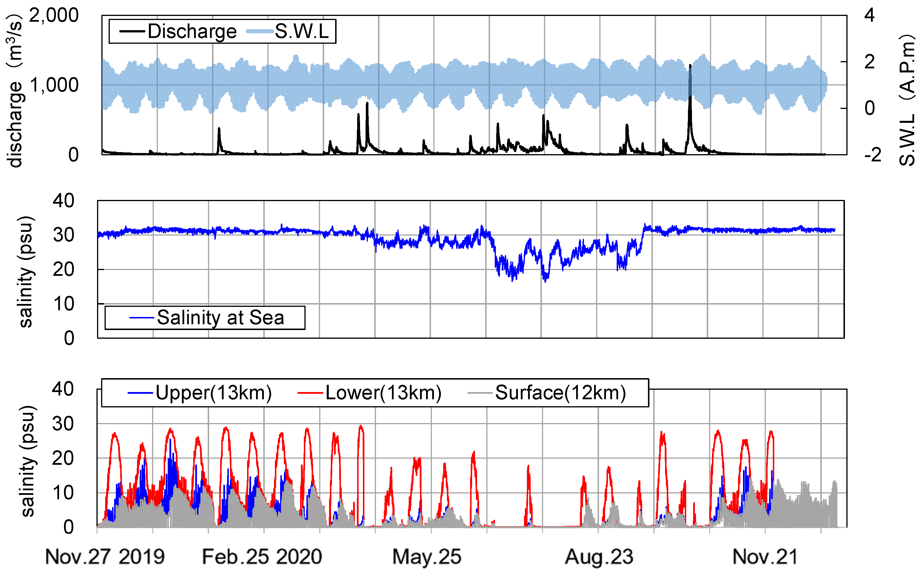
3.1. Water Salinity

The upper chart in Figure 9 shows the observed and calculated salinity levels at St. A and B in the month of January 2020. The lower charts show the salinity levels on neap, middle, and spring tide days. “Cal. (St. A)” is the salinity calculated from the shallow water model using the salinity and water level data obtained at St. B. The values dropped to zero once a day when the instruments dried out around the time of ebb tide, and the envelope line roughly corresponded to the tidal variation. The M2-constituent of the half-day period dominates in the Tokyo Bay, where the mouth of Arakawa River is located, and the amplitude variation of the two-week period according to the Moon age is also large. Note, however, that the water salinity in the marsh peaked in around the middle-tide, possibly as a consequence of the decreased seawater intrusion distance from Tokyo Bay on spring-tide days resulting from the enhanced vertical mixing. The calculated salinity at St. A almost agreed with the measured value. The error value of residual mean is 0.24 psu.

The color maps in Figure 10 show the numerical simulation results for water salinity variations in the marsh on neap, middle and spring-tide days. The period covered in the simulation is marked on the water level plots on the left, recorded at St. B. The water area expands from the central pond to the salt marsh, and the variation depends on the tidal fluctuation, ranging from lowest on the neap-tide day to highest on the spring-tide day. Note that the highest salinity appears on the middle-tide day.

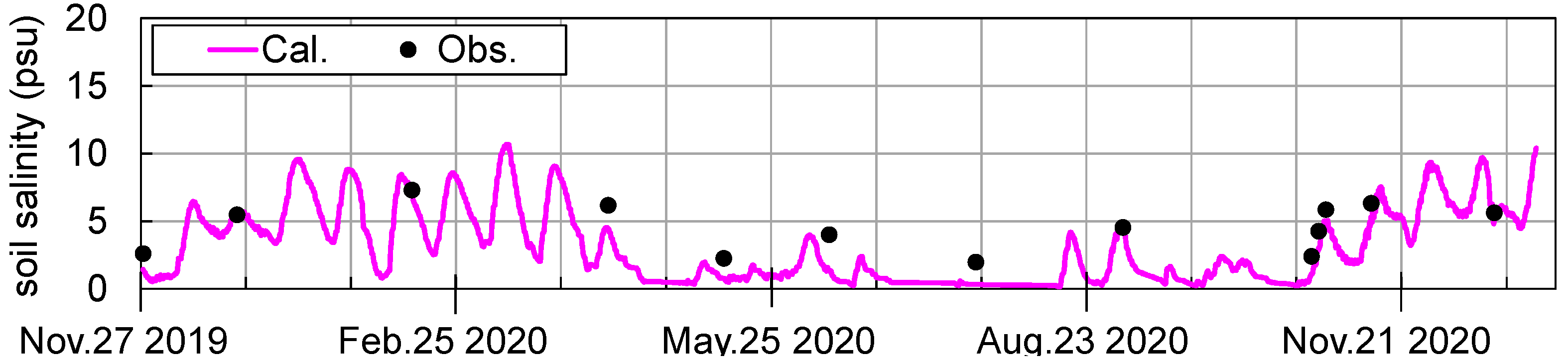
3.2. Soil Salinity and Hydraulic Conductivity

Figure 11 shows the calculated result of soil salinity. Here the water salinity $S_0\left(t\right)$ was given as the observed salinity at St. B only, as the instrument at St. A. failed to take measurements for a full year. As shown in Figure 6, the salinities of St. A and St. B are almost the same over the period when the observation data are available. This correspondence in the salinities can presumably be explained by the small capacity of the Gotanno-wand, which results in an almost full exchange of the water by a single tide. In the verification of the model, the empirical constant γ was 1.0 × 10⁻⁵ (1/s) based on the reproducibility with the observed salinity. The observed salinity is plotted as the average value of all layers. From above, the reproducibility of the whole year, including the flood period, was secured. In addition, as we see in Figure 11, the calculated results conformed with the rapid salt fluctuations observed every two days in October. These results show that our model faithfully reproduces the vertical and horizontal salt movements attributed to the burrows of organisms, and can calculate the movements throughout the year. The error value of residual mean is −1.1 psu.

4. Discussion

4.1. Mechanism of Variation of Water Salinity

In Arakawa river, it has been reported that salt water runs up due to weak mixing at neap-tide days and strong mixing at spring-tide days [21]. As Figure 6 shows, the variation of salinity between the neap-tide days, middle-tide days, and spring-tide days can be explained by the following processes. First, during the neap-tide days, stratification is promoted as the tidal amplitude decreases, which leads to increasing salinity at the lower layer and decreasing salinity at the surface. Next, vertical mixing becomes active in the middle-tide days and intensifies in the spring-tide days, resulting in almost equal salinity at all layers. During the spring-tide days, the length of saltwater intrusion from the estuary decreases as the mixing intensifies, and the salinity decreases.

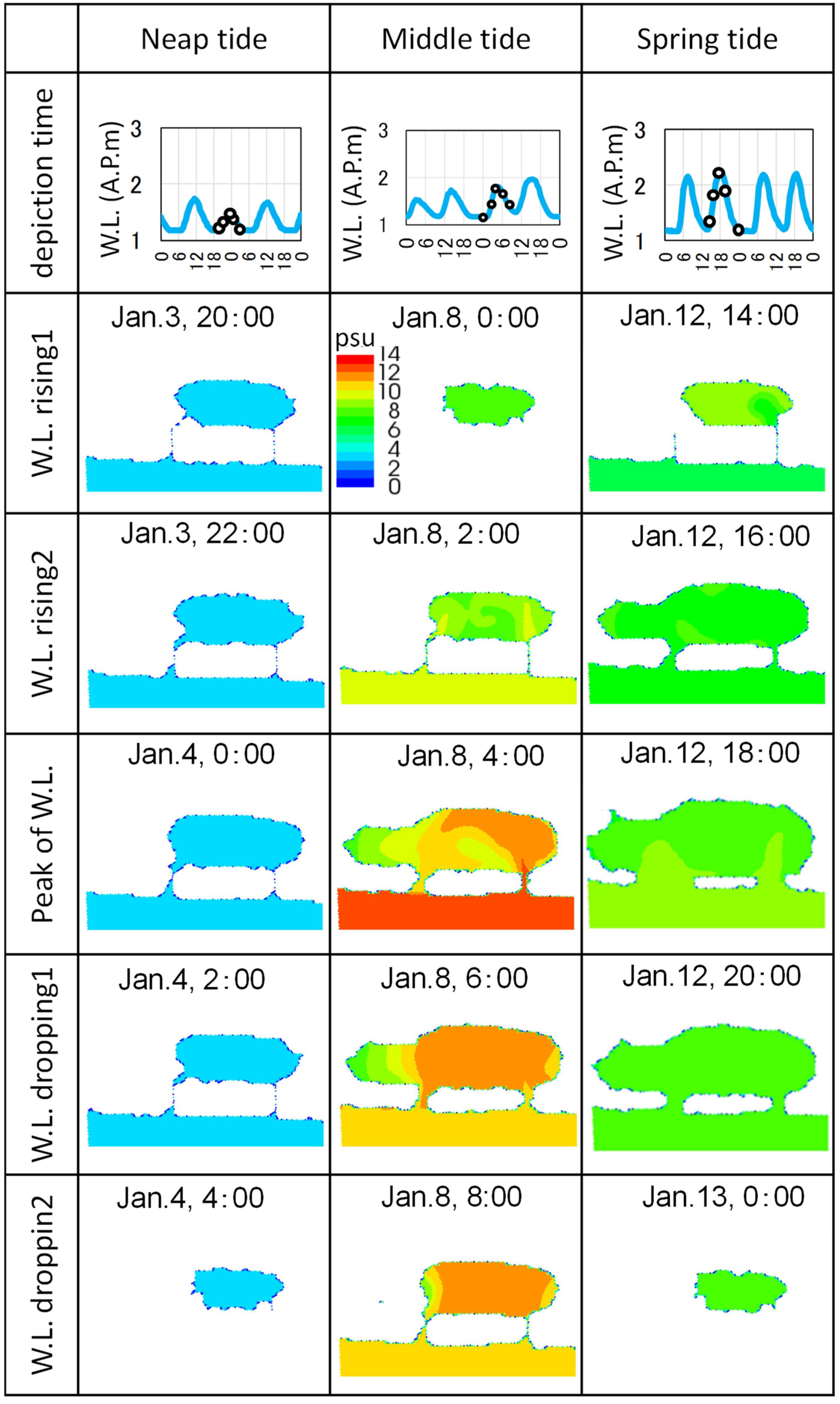
4.2. Pattern of Salt Supply to Soil at Marsh

Based on Figure 8 and the data on hydraulic conductivity, the pattern of the salt supply to the soil can be modeled as shown in Figure 12. The left and right image of Figure 12 show the pattern of the salt supply to the soil without and with the burrows left by organisms respectively. The salt water can quickly penetrate to at least the 40 cm layer through the burrows left by organisms. On the other hand, Lin et al. reported a case in which the roots of reeds contributed to salt penetration [5]. No reed roots were present, however, in the sample used for the hydraulic conductivity measurements in the present study. As such, we attribute the rapid penetration of salt water wholly to the burrows of crabs and worms.

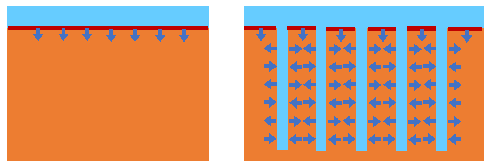
4.3. Mechanism of Salt Supply from Channel to Marsh to Marsh

Figure 11 shows the verification result when the observed salinity of St. B is given as the input data. Taking a different approach, the soil salinity at St. A can be estimated by the two-dimensional model shown in Figure 9. Ideally, the calculated results for the whole year should be given, but constraints in the calculation time compelled us to set the period to that covered in Figure 9. Figure 13 shows the calculated results of soil salinity. In order to consider the relationship with other items, the upper chart shows the tide level at Harumi (Tokyo Bay) and the discharge of the Akigase weir (35 km); the second chart, just below, shows the salinity at Urayasu point (Tokyo Bay); the third chart shows the salinity at the upper and lower layers of Nishiarai (13 km) and the salinity at St. B (12 km); the fourth chart shows the results calculated by the two-dimensional model; and the bottom chart shows the calculated soil salinity. We can see, from these charts, that the salinity at the lower layer at 13 km peaks in the neap-tide days, while that at the surface at 12 km peaks in the middle-tide days, with a delay (third chart). The observed salinity at St. B and the calculated salinity at St. A are almost the same (fourth chart), and the calculated soil salinity peaks later than the inundated water at St. A (comparison of the fourth and fifth charts). Further, we see that the observed data on 12 February can be reproduced (fifth chart). Though the salinity at the channel will fall sharply to almost zero because of the flood on 26 January, the soil salinity will fall gradually and stay at about 1psu (comparison of the fourth and fifth charts).

5. Conclusions

The marsh in Gotanno-wand is maintained in good condition as a brackish-water benthos habitat for two possible reasons. The first reason is the structure of the dike separating the marsh from the river channel. The porous materials composing the dike and shallow open flumes permit sufficient water exchange while protecting the marsh from water flow and waves in the river channel. The second reason is the soil salinity, which absorbs fluctuations in inundated salinity, partly through the infiltration of salinity into the soil through burrows formed by crabs and worms.

Finally, our results suggested that the shallow water model developed in this study can be combined with the soil salinity model to produce a design tool for the creation of a stable salt marsh.

References

- Keigo, N. River and Wetland Restoration. BioScience 2006, 56, 419–429. [Google Scholar]
- Bureau of Construction Tokyo. Bureau of Construction Overview 2012, Creating Our Future—Roads, Water, and Greenery; Bureau of Construction Tokyo: Nishishinjuku, Japan, 2012. [Google Scholar]
- Yodo River Office. The Yodo River Working Towards Fostering Confidence and Culture; Yodo River Office: Osaka, Japan, 2004. [Google Scholar]
- Lissner, J.; Schierup, H.H. Effects of salinity on growth of Phragmites australis. Aquat. Bot. 1997, 55, 247–260. [Google Scholar] [CrossRef]
- Qian, L.; Tadaharu, I.; Ryosuke, A.; Fenglin, Y.; Shushen, Z. Soil Salinity Reduction by River Water Irrigation in a Reed Field, A Case Study in Shuangtai Estuary Wetland, Northeast China. Ecol. Eng. 2016, 89, 32–39. [Google Scholar]
- McLusky, D.S. The Estuarine Ecosystem, 2nd ed.; Wiley-Blackwell: Hoboken, NJ, USA, 1999. [Google Scholar]
- Yonghai, S.; Genyu, Z.; Jianzhong, L.; Yazhu, Z.; Jiabo, X. Performance of a Constructed Wetland in Treating Brackish Wastewater from Commercial Recirculating and Super-intensive Shrimp Growout Systems. Bioresour. Technol. 2011, 102, 9416–9424. [Google Scholar]
- Heta, R.; Samuli, K.; Erik, B. Brackish-Water Benthic Fauna under Fluctuating Environmental Conditions: The Role of Eutrophication, Hypoxia, and Global Change. Front. Mar. Sci. 2019, 6, 1–13. [Google Scholar]
- Norouzi, M.; Bagheri, T.M. The Effects of Salinity, PH and Temperature Changes on the Macrobenthos of the Shirud River Deltaic Region (Caspian Sea. Northern Iran). In Proceedings of the 2nd International Congress on Applied Ichthyology & Aquatic Environment, Messolonghi, Greece, 10–12 November 2016; pp. 544–549. [Google Scholar]
- Colin, R.J.; Scarlett, C.V. Effects of salinity and nutrients on microbial assemblages in Louisiana wetland sediments. Wetlands 2009, 29, 277–287. [Google Scholar]
- Heather, G.; Nigel, W.T.Q. Comparison of Soil Salinity Analysis Methods for Wetland Soils; The U.S. Department of Energy and the U.S. Bureau of Reclamation and Department: Washington, DC, USA, 2004; pp. 1–11. [Google Scholar]
- Yuan, C.; Jingkuan, S.; Wenquan, L.; Jing, W.; Mengwei, Z. Mapping coastal wetland soil salinity in different seasons using an improved comprehensive land surface factor system. Ecol. Indic. 2019, 107, 105517. [Google Scholar] [CrossRef]
- Drew, N.F.; Sammy, L.K.; David, C.W. Evaluating Abiotic Influences on Soil Salinity of Inland Managed Wetlands and Agricultural Croplands in a Semi-Arid Environment. Wetlands 2014, 34, 1229–1239. [Google Scholar]
- Marcia, S.G.; Rondney, J.S. Subsurface Flow and Salinity Response Patterns in a Tidal Wetland Marsh Plain. J. Coast. Res. 2001, 27, 88–108. [Google Scholar]
- Gregg, E.M.; David, M.B.; Chris, R.P.; Donald, R.K. Mapping Soil Pore Water Salinity of Tidal Marsh Habitats Using Electromagnetic Induction in Great Bay Estuary, USA. Wetlands 2011, 31, 309–318. [Google Scholar]
- Juan, H.; David, C.W.; Carman, C. Two Fixed Ratio Dilutions for Soil Salinity Monitoring in Hypersaline Wetlands. PLoS ONE 2015, 10, e0126493. [Google Scholar] [CrossRef] [Green Version]
- Japanese Standards Association. Methods for Testing the Hydraulic Conductivity of Saturated Soils; JIS A 1218; Japanese Standards Association: Tokyo, Japan, 2020. [Google Scholar]
- Creager, W.P.; Justin, J.D.; Hinds, J. Engineering for Dams, Vol. III, Earth, Rock-Fill, Steel and Timber Dams; John, Wiley & Sons, Inc.: Hoboken, NJ, USA, 1945; pp. 645–649. [Google Scholar]
- Nagata, N. Numerical Analysis of Two-Dimensional Unsteady Flow on a General Coordinate System. In Proceedings of the Workshop on Using Computers in Water Engineering (Lecture Text), Kyoto University, Kyoto, Japan, August 1999. [Google Scholar]
- Japan Institute of Construction Engineering. Guide for the Study of River Channel Planning; Japan Institute of Construction Engineering: Tokyo, Japan, 2002; pp. 115–118. [Google Scholar]
- Yu, K.; Nerriza, O.; Yuta, U.; Katsuhide, Y. Effect of Saltwater Intrusion on Water Distribution in Arakawa and Sumidagawa Estuaries under Normal Conditions. J. JSCE Ser. B2 Coast. Eng. 2019, 75, I_205–I_210. [Google Scholar]
Publisher’s Note: MDPI stays neutral with regard to jurisdictional claims in published maps and institutional affiliations. |
© 2021 by the authors. Licensee MDPI, Basel, Switzerland. This article is an open access article distributed under the terms and conditions of the Creative Commons Attribution (CC BY) license (https://creativecommons.org/licenses/by/4.0/).
Share and Cite
Kuroda, N.; Yokoyama, K.; Ishikawa, T. Development of a Practical Model for Predicting Soil Salinity in a Salt Marsh in the Arakawa River Estuary. Water 2021, 13, 2054. https://doi.org/10.3390/w13152054
Kuroda N, Yokoyama K, Ishikawa T. Development of a Practical Model for Predicting Soil Salinity in a Salt Marsh in the Arakawa River Estuary. Water. 2021; 13(15):2054. https://doi.org/10.3390/w13152054
Chicago/Turabian StyleKuroda, Naoki, Katsuhide Yokoyama, and Tadaharu Ishikawa. 2021. "Development of a Practical Model for Predicting Soil Salinity in a Salt Marsh in the Arakawa River Estuary" Water 13, no. 15: 2054. https://doi.org/10.3390/w13152054
APA StyleKuroda, N., Yokoyama, K., & Ishikawa, T. (2021). Development of a Practical Model for Predicting Soil Salinity in a Salt Marsh in the Arakawa River Estuary. Water, 13(15), 2054. https://doi.org/10.3390/w13152054