
Estimation of Vegetation-Induced Flow Resistance for Hydraulic Computations Using Airborne Laser Scanning Data


Abstract
:1. Introduction
2. Methods for Quantification of Resistance
2.1. Resistance Formulas
2.2. Vegetation Parameter
2.3. Terrestrial Laser Scanning
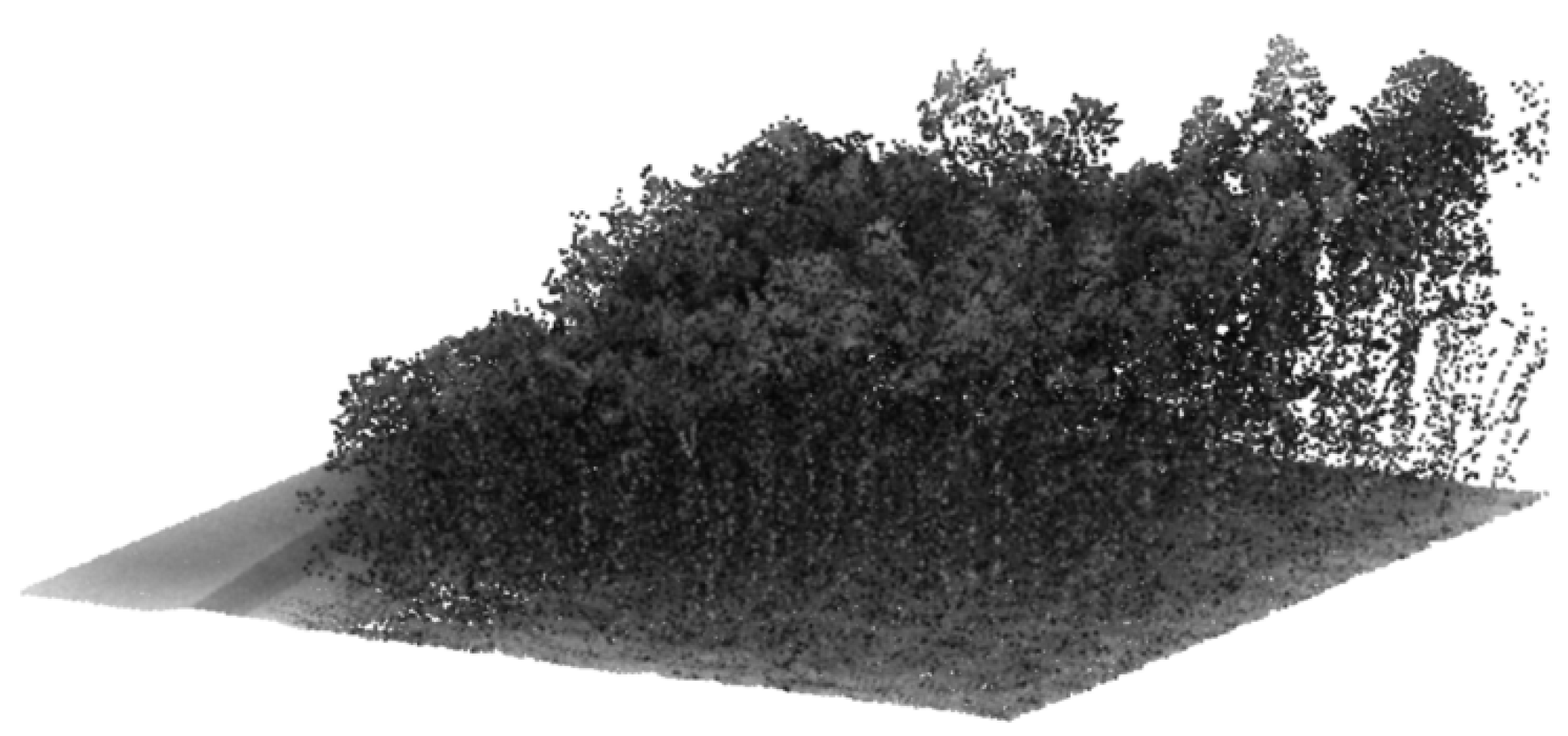
2.4. Airborne Laser Scanning
3. Procedure to Process ALS Data
3.1. Processing of the Laser Scanner Data
3.2. Full Waveform Laser Processing
3.3. Description of the Proposed Procedure
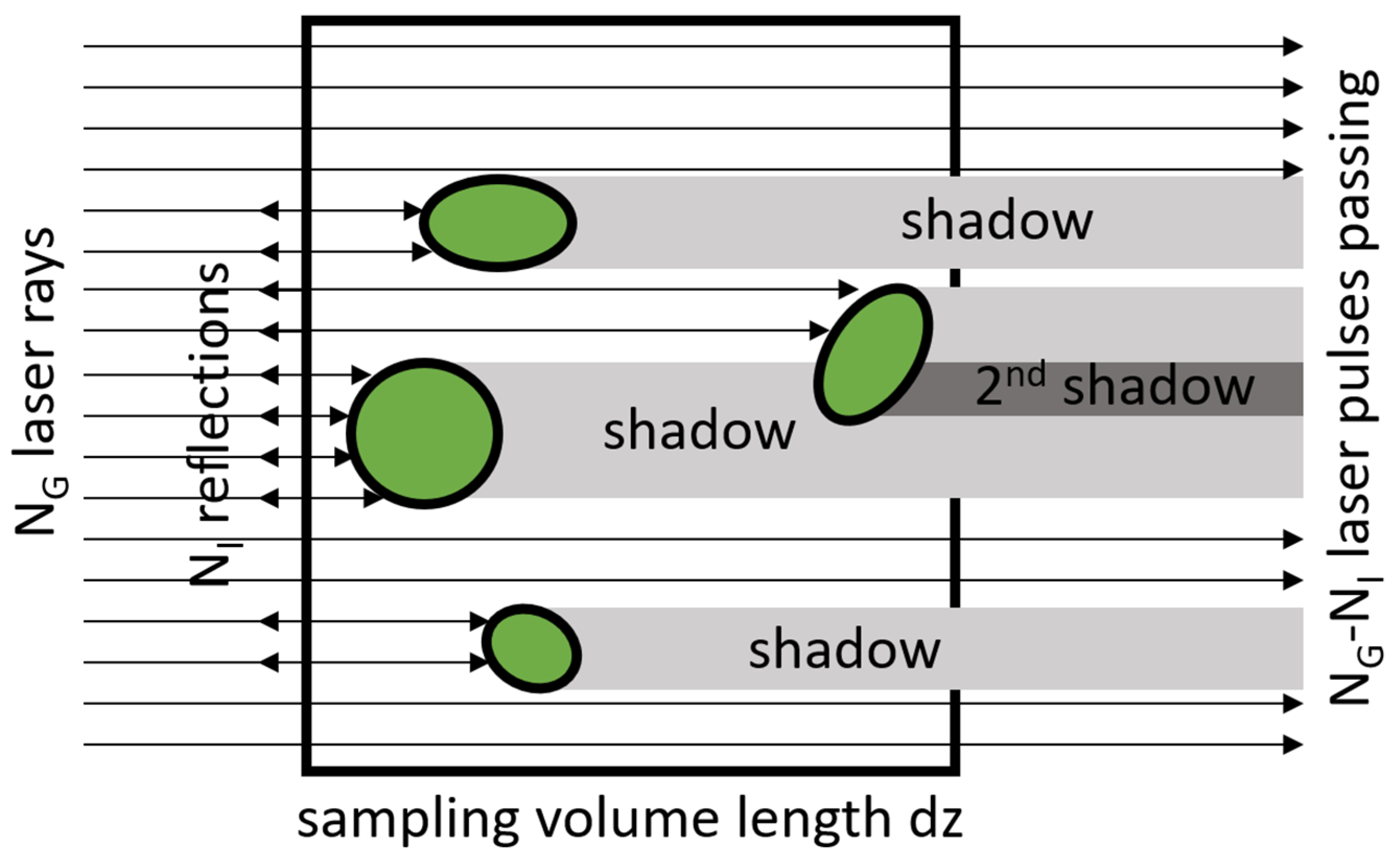
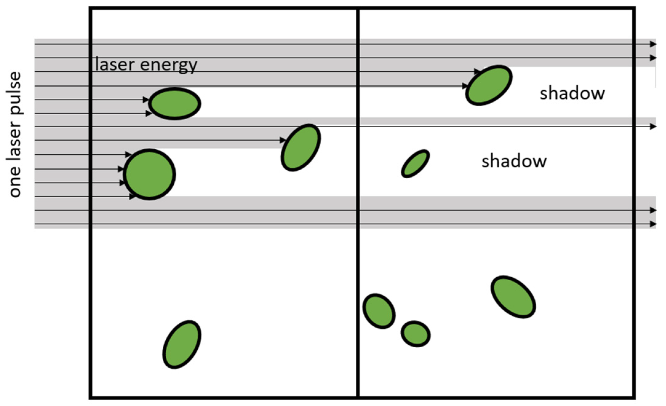
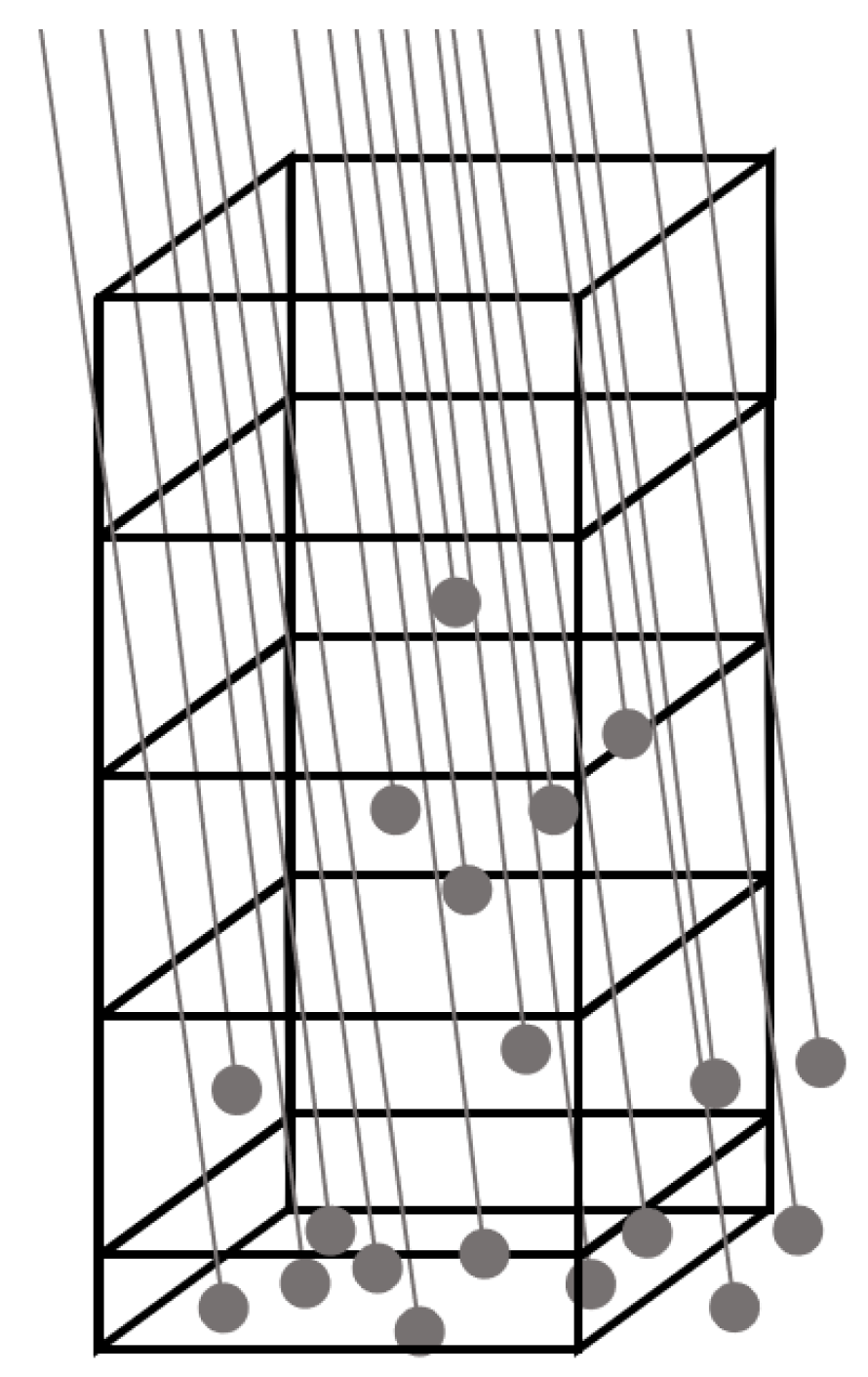
- The laser ray shedding is nearly parallel.
- The direction of the rays is nearly vertical downward; 20° in practice.
- The vertical projection and the horizontal projection of the vegetation area are the same.
- The number of reflection points of the laser rays divided by the number of imposed rays gives the area fraction of the vegetation inside each voxel.
- For each voxel, the number of reflexion points Ni is counted. Additionally, a ground box or voxel of different height may be defined, where the number of reflexion points is counted as well.
- Summing up the reflexion points from the ground vertically upwards to the top gives the number of test rays that entered a voxel column Nin, i at the top:
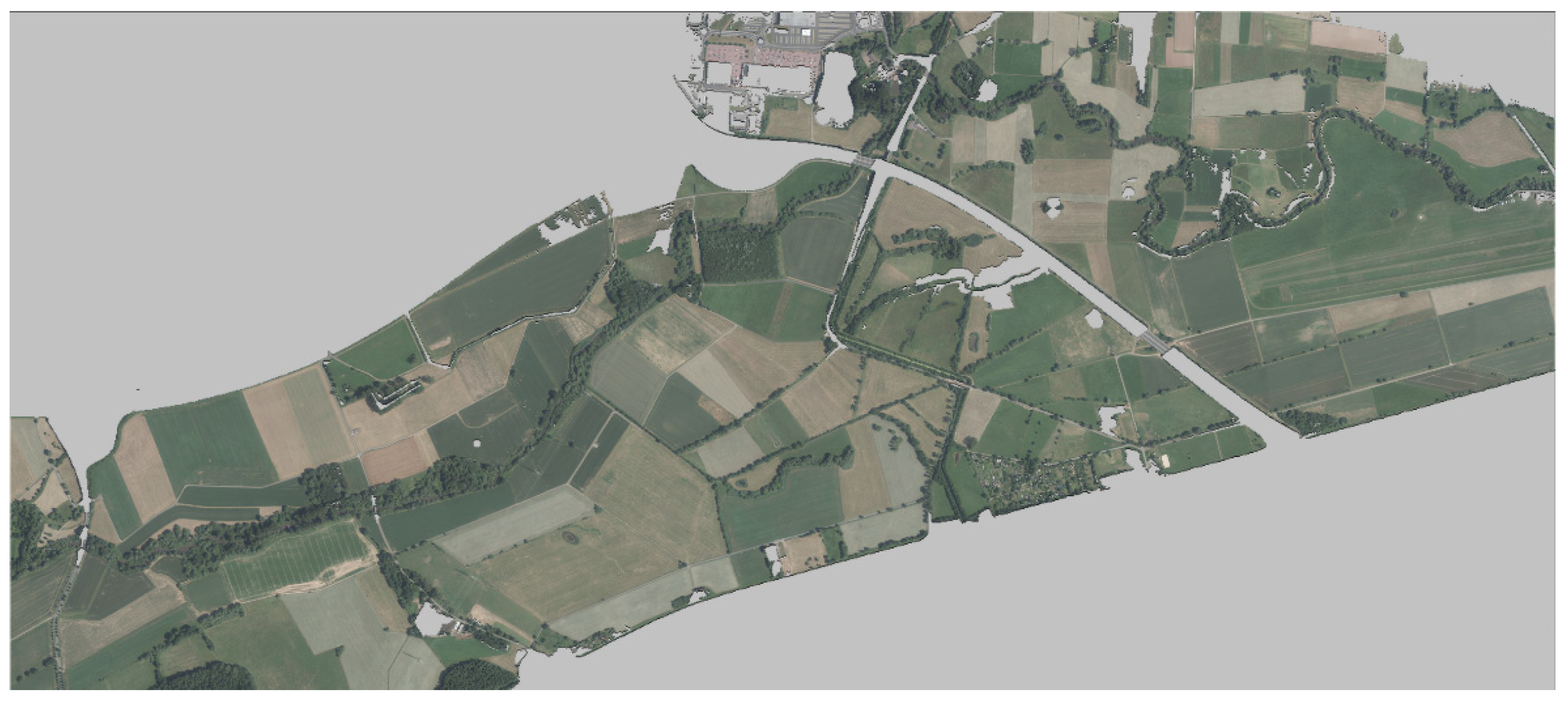
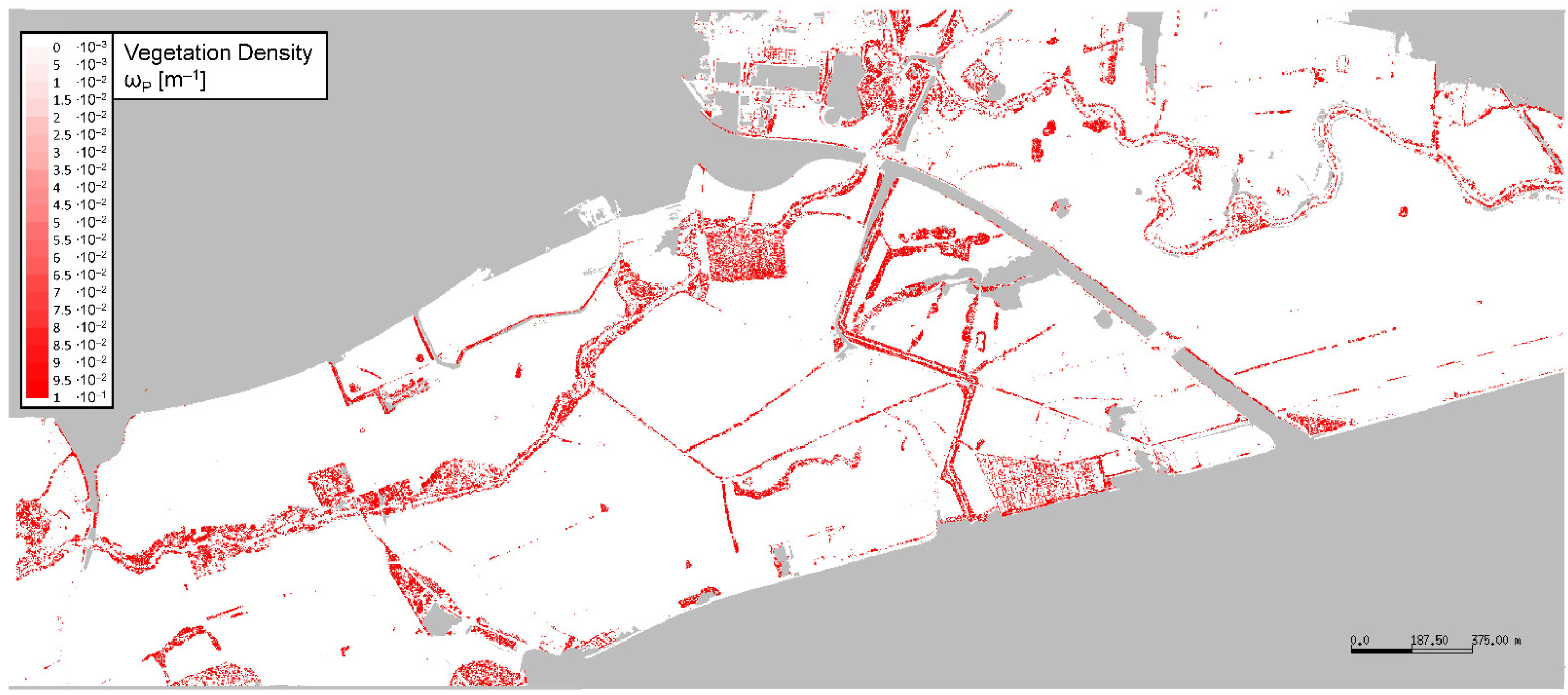
4. Case Study for the Kinzig Watercourse
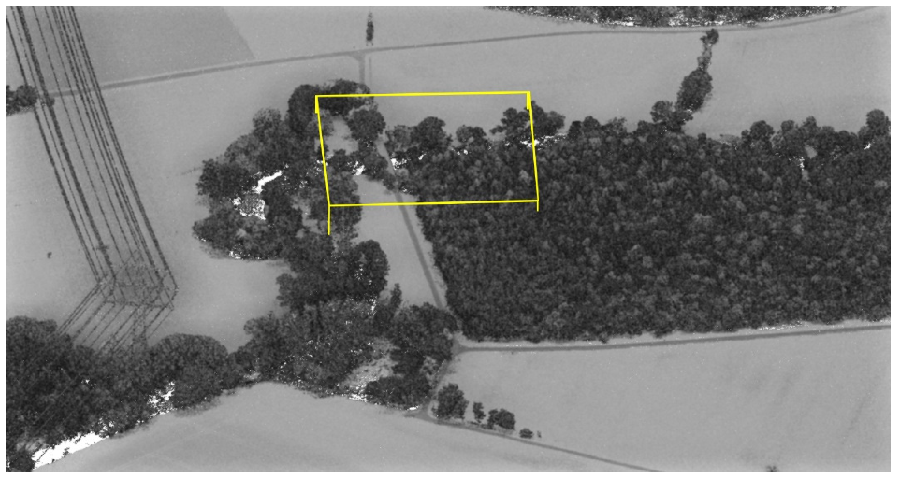
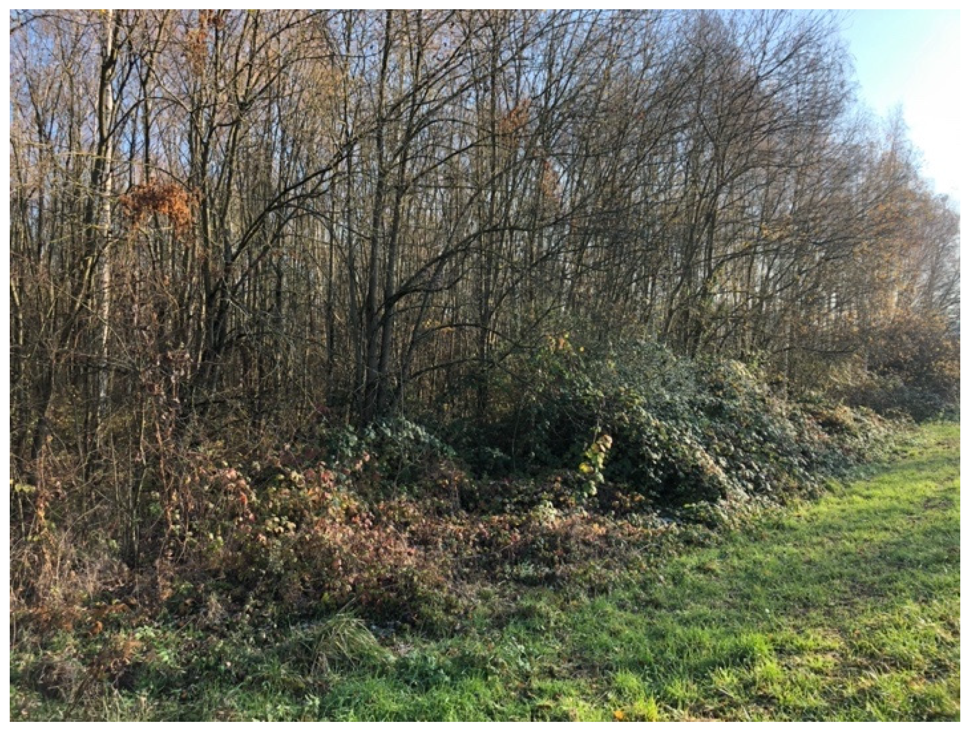
4.1. Study Area
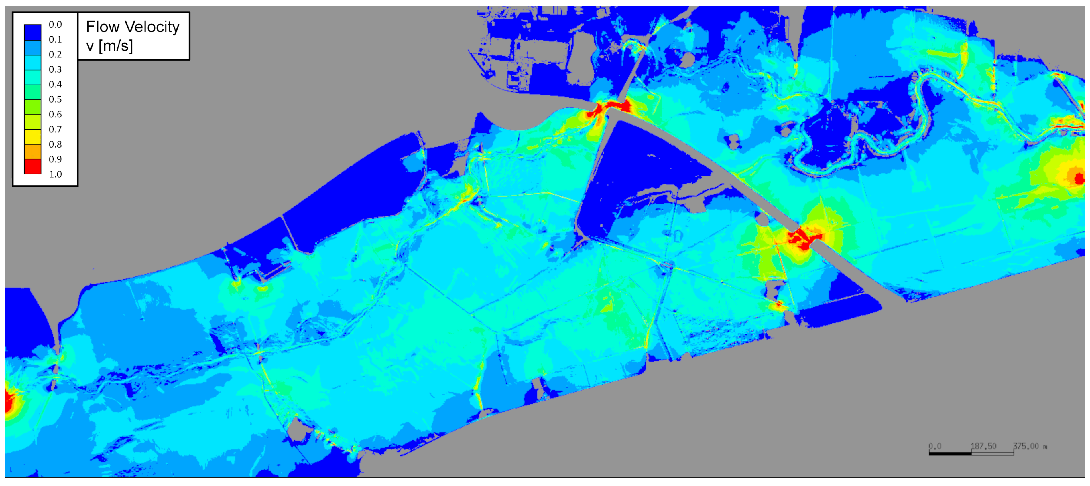
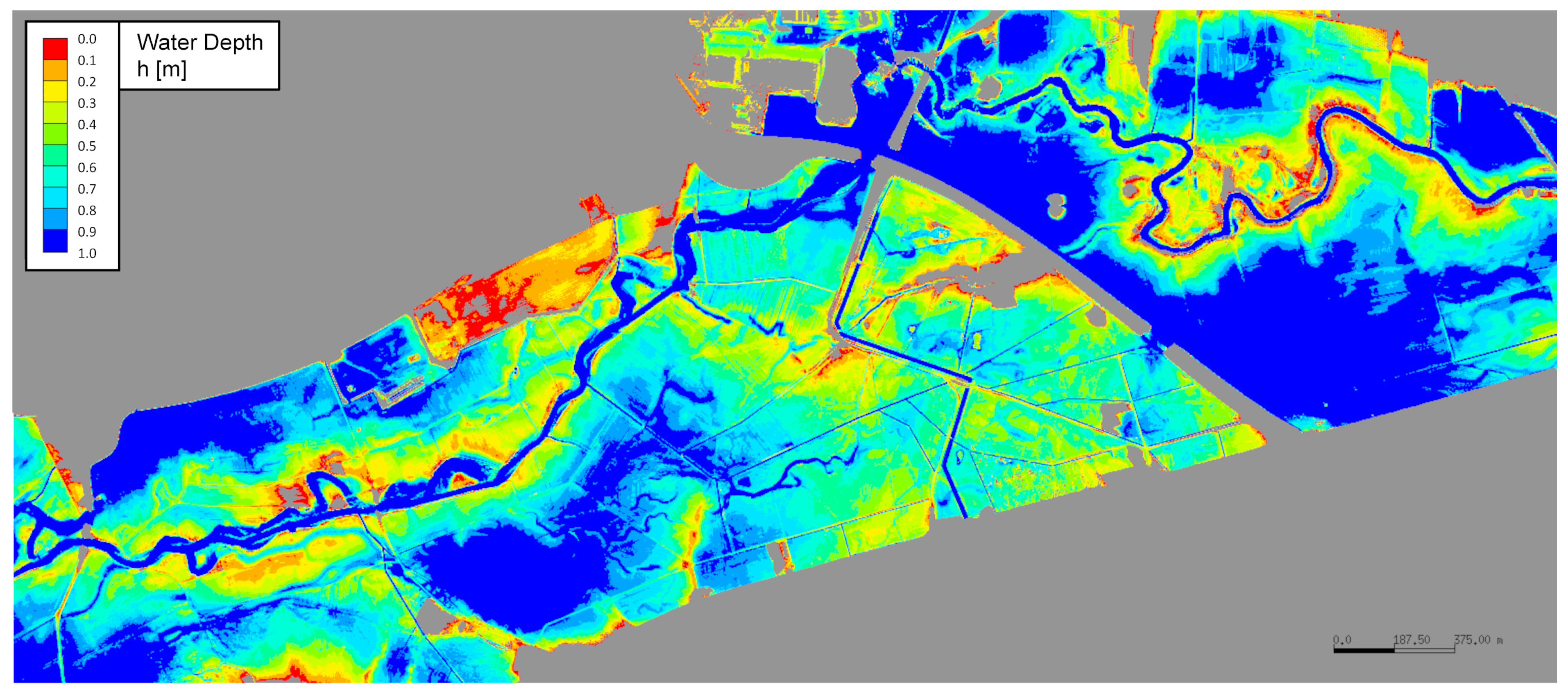
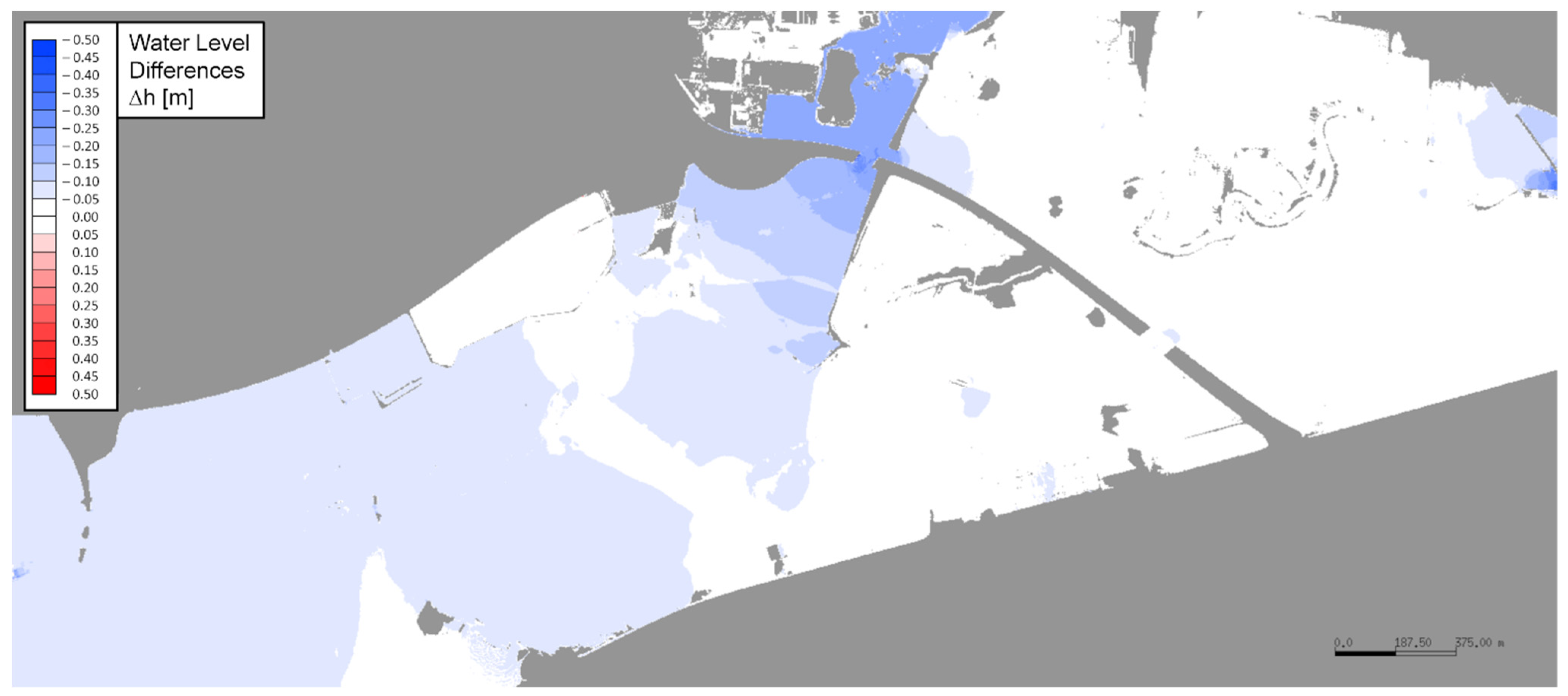
4.2. Flood Model Results
5. Conclusions
Funding
Informed Consent Statement
Data Availability Statement
Acknowledgments
Conflicts of Interest
References
- Arcement, G.J.; Schneider, V.R. Guide for Selecting Manning’s Roughness Coefficients for Natural Channels and Flood Plains; U.S. Geological Survey Water-Supply Paper 2339; U.S. Government Publishing Office: Washington, DC, USA, 1989.
- Järvelä, J. Determination of flow resistance caused by non-submerged woody vegetation. Int. J. River Basin Manag. 2004, 2, 61–70. [Google Scholar] [CrossRef]
- Straatsma, M.W.; Baptist, M.J. Floodplain roughness parameterization using airborne laser scanning and spectral remote sensing. Remote Sens. Environ. 2008, 112, 1062–1080. [Google Scholar] [CrossRef]
- Forzieri, G.; Castelli, F.; Preti, F. Advances in remote sensing of hydraulic roughness. Int. J. Remote Sens. 2012, 33, 630–654. [Google Scholar] [CrossRef]
- Luo, S.; Wang, C.; Pan, F.; Xi, X.; Li, G.; Nie, S.; Xia, S. Estimation of wetland vegetation height and leaf area index using airborne laser scanning data. Ecol. Indic. 2015, 48, 550–559. [Google Scholar] [CrossRef]
- Wang, C.; Zheng, S.; Wang, P.; Hou, J. Interactions between vegetation, water flow and sediment transport: A review. J. Hydrodyn. Ser. B 2015, 27, 24–37. [Google Scholar] [CrossRef]
- DFG-Forschungsbericht, Hydraulische Probleme beim Naturnahen Gewässerausbau; VCH-Verlagsgesellschaft: Weinheim, Germany, 1987.
- Lindner, K. Der Strömungswiderstand von Pflanzenbeständen, Mitteilung des Leichtweiss-Institut für Wasserbau, Heft 75; Leichtweiss-Inst. für Wasserbau: Braunschweig, Germany, 1982. [Google Scholar]
- DVWK Heft 220, Hydraulische Berechnung von Fließgewässern, Merkblatt zur Wasserwirtschaft; Deutsche Vereinigung für Wasserwirtschaft, Abwasser und Abfall: Hamburg/Berlin, Germany, 1991.
- Bretschneider, H.; Schulz, A. Anwendung von Fließformeln bei Naturnahem Gewässerausbau, Schriftenreihe des DVWK, Heft 72; Verlag Paul Parey: Hamburg, Germany, 1985. [Google Scholar]
- BWK. Hydraulische Berechnung von Naturnahen Fließgewässern—Teil 2; Bund der Ingenieure für Wasserwirtschaft, Abfallwirtschaft und Kulturbau (BWK e.V.): Pfullingen, Germany, 2000. [Google Scholar]
- Mewis, P. Numerische Berechnungen zum Einfluss Verschiedener Bewuchsstadien auf das Fließgeschehen, Darmstädter Wasserbauliches Kolloquium 1996. In Mitteilungen des Institutes für Wasserbau; Heft 98; TU-Darmstadt: Darmstadt, Germany, 1997; pp. 237–249. [Google Scholar]
- Petryk, S.; Bosmajian, G. Analysis of flow through vegetation. J. Hydr. Div. ASCE 1975, 101, 871–884. [Google Scholar] [CrossRef]
- Zahidi, I.; Yusuf, B.; Cope, M.; Mohamed, T.A.; Shafri, H.Z.M. Effects of depth-varying vegetation roughness in two-dimensional hydrodynamic modelling. Int. J. River Basin Manag. 2018, 16. [Google Scholar] [CrossRef]
- Jalonen, J.; Järvelä, J.; Aberle, J. Leaf Area Index as Vegetation Density Measure for Hydraulic Analyses. J. Hydraul. Eng. 2013, 139. [Google Scholar] [CrossRef]
- Luhar, M.; Nepf, H.M. Flow-induced reconfiguration of buoyant and flexible aquatic vegetation. Limnol. Oceanogr. 2011, 56, 2003–2017. [Google Scholar] [CrossRef] [Green Version]
- Schoneboom, T. Widerstand Flexibler Vegetation und Sohlenwiderstand in durchströmten Bewuchsfeldern. Ph.D. Dissertation, TU Braunschweig, Braunschweig, Germany, 2011. [Google Scholar]
- Stephan, U.; Gutknecht, D. Hydraulic resistance of submerged flexible vegetation. J. Hydrol. 2002, 269, 27–43. [Google Scholar] [CrossRef]
- Stephan, U. Zum Fließwiderstandsverhalten Flexibler Vegetation. Wiener Mitteilungen des Instituts für Hydraulik, Gewässerkunde und Wasserwirtschaft; Band 180; Technische Universität Wien: Wien, Germany, 2002. [Google Scholar]
- Västilä, K.; Järvelä, J. Modeling the flow resistance of woody vegetation using physically based properties of the foliage and stem. Water Resour. Res. 2014, 50, 229–245. [Google Scholar] [CrossRef]
- Schneider, S. Widerstandsverhalten von holzigen Auenpflanzen—Konzept zur Etablierung von Weichholzauen an Fließgewässern. Ph.D. Dissertation, Karlsruher Institut für Technologie (KIT), Karlsruhe, Germany, 2010. [Google Scholar]
- Wunder, S. Zum Fließverhalten um strauchartige Weidengewächse und dessen Auswirkungen auf den Strömungswiderstand. Ph.D. Dissertation, Universität Karlsruhe KIT, Karlsruhe, Germany, 2014. [Google Scholar]
- Hartlieb, A. Modellversuche zur Rauheit durch- bzw. überströmter Maisfelder, Wasserwirtschaft, Nr. 3/2006; Wasserwirtschaft: Wiesbaden, Germany, 2006; pp. 38–41. [Google Scholar]
- Habersack, H. Zusammenstellung von kst-Rauheitsbeiwerten, BOKU Wien. Available online: http://iwhw.boku.ac.at/LVA816332/Flie%E1widerstand_Einheit_5.pdf (accessed on 12 March 2018).
- Antonarakis, A.S.; Richards, K.S.; Brasington, J.; Muller, E. Determining leaf area index and leafy tree roughness using terrestrial laser scanning. Water Resour. Res. 2010, 46, W06510. [Google Scholar] [CrossRef] [Green Version]
- Wohlfahrt, G.; Sapinsky, S.; Tappeiner, U.; Cernusca, A. Estimation of plant area index of grasslands from measurements of canopy radiation profiles. Agric. For. Meteorol. 2001, 109, 1–12. [Google Scholar] [CrossRef]
- Oplatka, M. Stabilität von Weidenverbauungen an Flussufern; Heft 156; Mitteilungen der Versuchsanstalt für Hydrologie und Glaziologie der Eidgenössischen Technischen Hochschule: Zürich, Switzerland, 1998. [Google Scholar]
- Toda, M.; Richardson, A.D. Estimation of plant area index and phenological transition dates from digital repeat photography and radiometric approaches in a hardwood forest in the Northeastern United States. Agric. For. Meteorol. 2018, 249, 457–466. [Google Scholar] [CrossRef]
- Ogunbadewa, E.Y. Tracking seasonal changes in vegetation phenology with a SunScan canopy analyzer in northwestern England. For. Sci. Technol. 2012, 8, 161–172. [Google Scholar] [CrossRef]
- Peduzzi, A.; Wynne, R.H.; Fox, T.R.; Nelson, R.F.; Thomas, V.A. Estimating leaf area index in intensively managed pine plantations using airborne laser scanner data. For. Ecol. Manag. 2012, 270, 54–65. [Google Scholar] [CrossRef] [Green Version]
- Parker, G.; Harding, D.J.; Berger, M.L. A portable LIDAR system for rapid determination of forest canopy structure. J. Appl. Ecol. 2004, 41, 755–767. [Google Scholar] [CrossRef]
- Hosoi, F.; Omasa, K. Voxel-Based 3-D Modeling of Individual Trees for Estimating Leaf Area Density Using High-Resolution Portable Scanning Lidar. IEEE Trans. Geosci. Remote Sens. 2006, 44, 12. [Google Scholar] [CrossRef]
- Jalonen, J.; Järvelä, J.; Virtanen, J.-P.; Vaaja, M.; Kurkela, M.; Hyyppä, H. Determining Characteristic Vegetation Areas by Terrestrial Laser Scanning for Floodplain Flow Modeling. Water 2015, 7, 420–437. [Google Scholar] [CrossRef] [Green Version]
- Blair, J.B.; Rabine, D.L.; Hofton, M.A. The Laser Vegetation Imaging Sensor: A medium-altitude, digitisation-only, airborne laser altimeter for mapping vegetation and topography. ISPRS J. Photogramm. Remote Sens. 1999, 54, 115–122. [Google Scholar] [CrossRef]
- Lovell, J.L.; Jupp, D.L.B.; Culvenor, D.S.; Coops, N.C. Using airborne and ground-based ranging lidar to measure canopy structure in Australian forests. Can. J. Remote Sens. 2003, 29, 607–622. [Google Scholar] [CrossRef]
- Fewtrell, T.J.; Duncan, A.; Sampson, C.C.; Neal, J.C.; Bates, P.D. Benchmarking urban flood models of varying complexity and scale using high resolution terrestrial LiDAR data. Phys. Chem. Earth 2011, 36, 281–291. [Google Scholar] [CrossRef]
- Wessels, M.; Brückner, N.; Gaide, S.; Wintersteller, P. Tiefenschärfe—Die Hochauflösende Vermessung des Bodensees; Wasserwirtschaft: Wiesbaden, Germany, 2017; Volume 4. [Google Scholar]
- de Almeida, D.R.A.; Stark, S.C.; Shao, G.; Schietti, J.; Nelson, B.W.; Silva, C.A.; Gorgens, E.B.; Valbuena, R.; de Almeida Papa, D.; Brancalion, P.H.S. Optimizing the Remote Detection of Tropical Rainforest Structure with Airborne Lidar: Leaf Area Profile Sensitivity to Pulse Density and Spatial Sampling. Remote Sens. 2019, 11, 92. [Google Scholar] [CrossRef] [Green Version]
- Wagner, W.; Ullrich, A.; Melzer, T.; Briese, C.; Kraus, K. From Single-Pulse to Full-Waveform Airborne Laser Scanners: Potential and Practical Challenges. 2004. Available online: https://publik.tuwien.ac.at/files/PubDat_119591.pdf (accessed on 1 July 2021).
- Wagner, W.; Ullrich, A.; Briese, C. Der Laserstrahl und Seine Interaktion mit der Erdoberfläche. 2004. Available online: https://publik.tuwien.ac.at/files/PubDat_119558.pdf (accessed on 1 July 2021).
- MacArthur, R.H.; Horn, H.S. Foliage profile by vertical measurements. Ecology 1969, 50, 802–804. [Google Scholar] [CrossRef] [Green Version]
- Mewis, P. Sparse element for shallow water wave equations on triangle meshes. Int. J. Numer. Methods Fluids 2013, 72, 864–882. [Google Scholar] [CrossRef]


| [m−1] | [–] | Flow velocity [m/s] for slope S = 1.5‰ | [–] | ||
| h = 1 m | h = 0.5 m | ||||
| 0.01 | 0.048 | 40.4 | 1.56 | 0.024 | 80.8 |
| 0.03 | 0.144 | 23.3 | 0.90 | 0.072 | 46.7 |
| 0.1 | 0.48 | 12.8 | 0.49 | 0.24 | 25.6 |
| 1 | 4.8 | 4.0 | 0.16 | 2.4 | 8.1 |
Publisher’s Note: MDPI stays neutral with regard to jurisdictional claims in published maps and institutional affiliations. |
© 2021 by the author. Licensee MDPI, Basel, Switzerland. This article is an open access article distributed under the terms and conditions of the Creative Commons Attribution (CC BY) license (https://creativecommons.org/licenses/by/4.0/).
Share and Cite
Mewis, P. Estimation of Vegetation-Induced Flow Resistance for Hydraulic Computations Using Airborne Laser Scanning Data. Water 2021, 13, 1864. https://doi.org/10.3390/w13131864
Mewis P. Estimation of Vegetation-Induced Flow Resistance for Hydraulic Computations Using Airborne Laser Scanning Data. Water. 2021; 13(13):1864. https://doi.org/10.3390/w13131864
Chicago/Turabian StyleMewis, Peter. 2021. "Estimation of Vegetation-Induced Flow Resistance for Hydraulic Computations Using Airborne Laser Scanning Data" Water 13, no. 13: 1864. https://doi.org/10.3390/w13131864
APA StyleMewis, P. (2021). Estimation of Vegetation-Induced Flow Resistance for Hydraulic Computations Using Airborne Laser Scanning Data. Water, 13(13), 1864. https://doi.org/10.3390/w13131864