1. Introduction
An anomaly detection is an identification of data points that behave differently from normal patterns, see [
1]. This process is essential as anomalous data can indicate changes in typical behaviors or technical malfunctions. After successfully detecting anomalies, a data imputation for substituting detected points or missing values is required. A significant amount of previous work has been performed in the area of the outlier detection for temporal data as thoroughly reviewed in [
2,
3,
4,
5,
6,
7,
8]. In the context of time series, input data are generally either univariate, which is our focus in this work, or a multivariate type. Both statistical and machine learning approaches were regularly applied for detecting anomalies as broadly reviewed in [
9,
10,
11,
12].
Detecting anomalies based on a prediction interval constructed from standard deviations spanning over the mean is one of a common practice. Instead of using the mean as the outlier indicator, various median-based methods were alternatively proposed due to their robustness [
13,
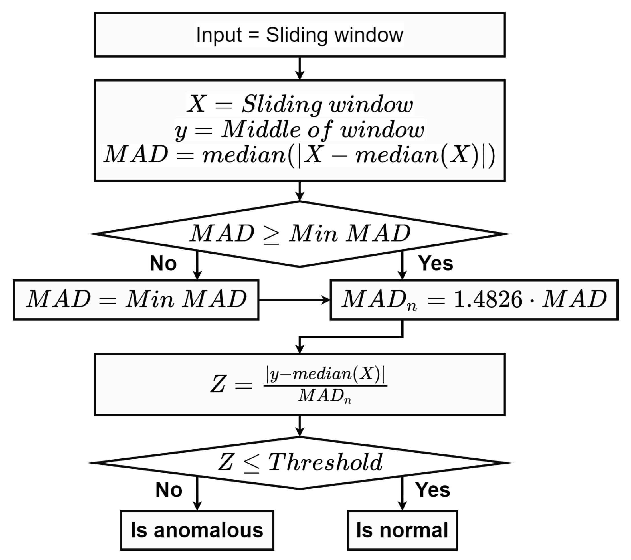
14]. Particularly, robust statistical metrics, median, and median absolute deviation (MAD), were introduced to accurately detect anomalies in [
15]. The MAD scale estimation is commonly used for the anomaly analysis due to its desirable performance. It is insensitive to a large dispersion of anomalous. Additionally, it is easy to implement and only a light computational effort is required [
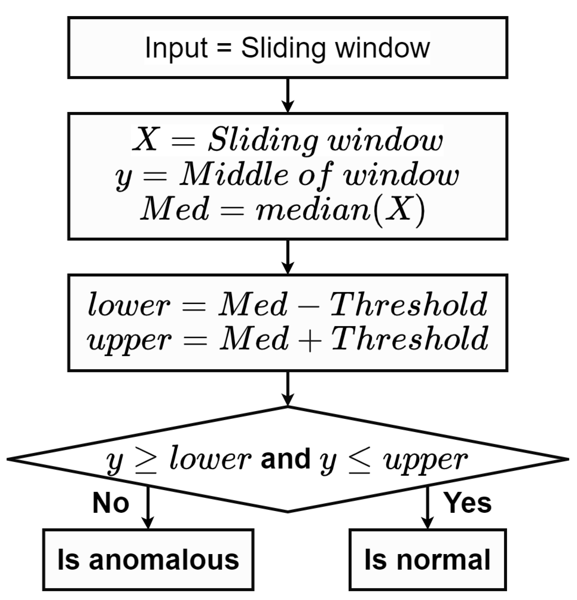
16]. Another important statistical-based method is the prediction confidence interval which relies on neighboring data to identify time series anomalies. An observed value is classified as anomalous if it falls outside of the range with upper and lower bounds of the interval [
17]. Its main advantage includes a capability to provide an automatic threshold for differentiate between normal and abnormal groups. Due to contrasting data distributions among various sources, a parameter tuning and a threshold estimation of the interval are the main challenges where further studies are highly required.
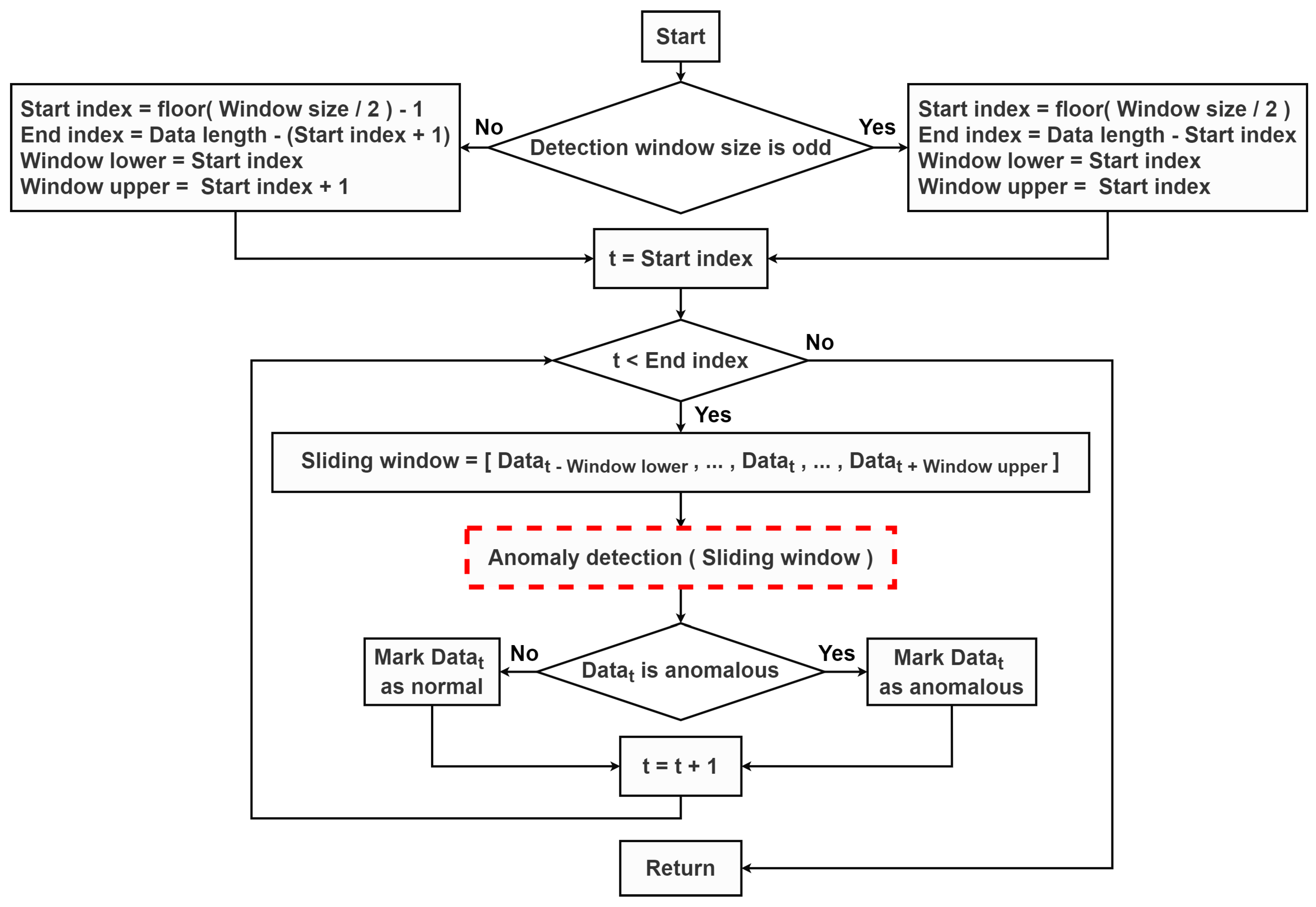
In order to detect anomalous points in time series, a sliding window technique is one of the powerful method due to its applicability for a real-time detection. It is commonly employed to sequentially detect outliers within a specific focus range over the raw data. It can be utilized with various outlier prediction methods without extensive modification. For instance, Yu et al. [
18] adopted the sliding window technique to segment the original hydrological time series into sub-sequences and further implemented an autoregressive prediction model with the prediction confidence interval to specify outlier points. Similar techniques were also applied in [
19] to identify outliers which were further corrected on meteorological data efficiently. In addition, the moving window was seamlessly implemented with the MAD scale estimator, as proposed in [
16]. According to the interpolation perspective, multiple data filling methods, such as a simple interpolation, a regression, an autoregressive and machine learning methods were introduced [
20]. In recent years, a deep learning method has been successfully applied to various tasks in time series analysis. In particular, a recurrent neural network (RNN), a specific type of deep learning models known to work well with temporal sequence data, have widely been used for the data imputation [
21]. Several studies also relied on a bidirectional RNN-based imputation to capture temporal information embedded in the original time series and further compute substituted values [
22,
23,
24].
In a water management system, hydrological time series are automatically collected from sensors at telemetry stations. Many environmental factors in surroundings such as floating objects or human operations can interfere the recorded values. These situations consequently result in anomalous points in the collected water level data. Poor-quality data potentially leads to incorrect implications and misleading insights. Therefore, the anomaly detection and the data imputation of identified anomalies or missing values for time series data are the necessary processes for any application in the water management analytics. Previous studies applied several techniques to detect anomaly patterns in hydrological time series. Yu et al. [
18] initially utilized the sliding window technique with an auto-regressive outlier prediction. Similarly, the ARIMA model with the confidence interval was employed with the moving window in [
25]. Various machine learning models were extensively implemented for the anomaly detection, such as a density-based approach [
26], SVM-based models [
27,
28], and the isolation forest algorithm [
29,
30]. The imputation methods for hydrological data processing, such as a simple infilling, a model-based deterministic, as well as machine learning methods were also explored [
31,
32]. With advanced deep learning models, Ren et al. [
33] relied on LSTM to complete gaps in spatial-temporal hydrological data.
A quality control method for hydrological data which included two forecasting models and one statistical model was proposed [
34]. Specifically, these proposed models were used to compute confidence intervals to detect potential outliers, as well as suggest proper values to fill suspicious and missing values. Bae and Ji [
35] developed a statistical process for detecting and removing anomalous data points of water level data from ultrasonic sensors. The modified Z-scores based on the MAD formula was applied for the anomaly detection process. Moreover, the detected data were further smoothed by an exponentially weighted moving average (EWMA) method. These two studies, which are the main motivation of our work, proposed a framework for the anomaly detection and the interpolation in order to process hydrological time series data.
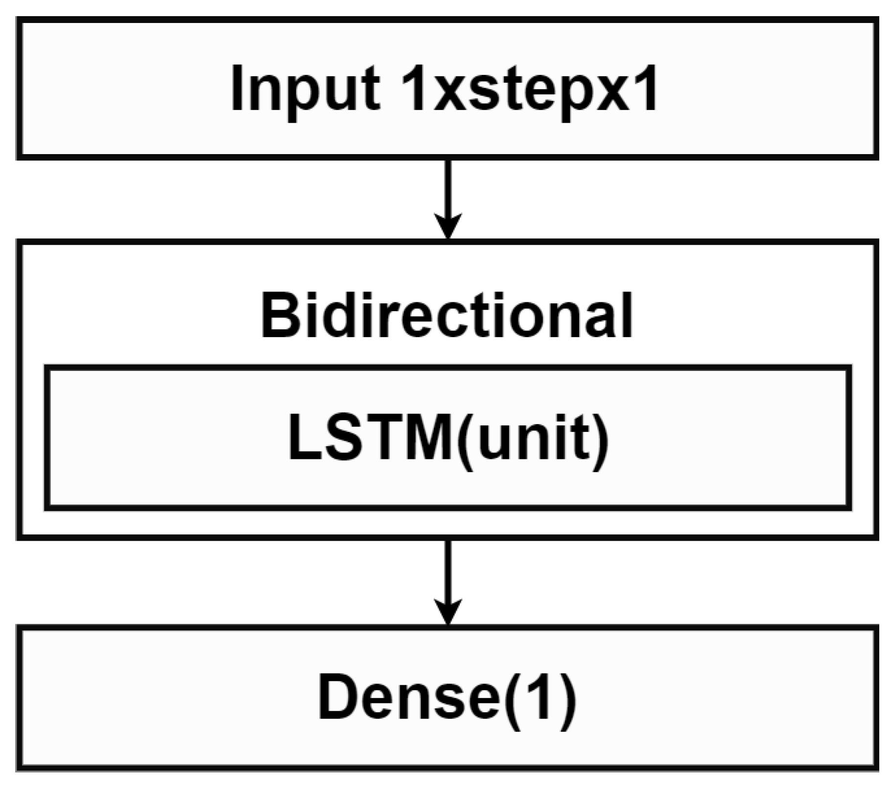
In this work, we focus on identifying data instances that deviated from normal data patterns. Technical anomalies based on an automatic sensor measurement are specifically considered both in terms of irregular quantities and frequency. We proposed a combination of MAD and the sliding window technique to capture irregular data behaviors in a specific time frame. Hence, anomaly points were detected locally over a specified window using the prediction interval. With a statistical characteristic of MAD, a superior performance was achieved especially with a large amount of data. In addition, missing values and anomalies were filled by various model predictions based on a sequence or an isolate point of anomalous data in the time window. Although the simple linear interpolation replaced missing values with a fitted linear line, the spline method relied on different polynomial sub-functions instead. Lastly, we employed the bidirectional LSTM model [
21], a weighted combination of a forward and a backward LSTM model, with a capability of learning an ordered dependency among sequential data. A main contribution of this work is exploring anomaly detection and data imputation of the overall data monitoring system with diverse data behaviors.
This work is under the project titled “Data analytics for improving the efficiency of water management: phase I” initiated for improving the data quality control from telemetry stations in Thailand. We retrieved water level time series from hydro-informatics institute (HII) as a case study. In order to evaluate the proposed methods, test cases were specifically constructed based on 2-year data of 4 telemetry stations with relatively complete data. We artificially manipulated 10% of the second-year data of each station with anomalies. The proposed anomaly detection were evaluated based on the manually-created anomalous data with F1-score. The prediction accuracy of the data filling methods is further measured using RMSE. A comparison based on predictability of all presented methods was performed.
The paper is organized as follows. A main methodology regarding backgrounds, anomaly detection methods, and data filling methods are described in
Section 2.
Section 3 discusses an experimental analysis consisting of a data preparation for our case studies, parameters, training configurations, as well as evaluation metrics. Results and discussions are provided in
Section 4 while the conclusion are summarized in
Section 5.
3. Experimental Analysis
In this section, our case studies regarding hydrological time series are discussed. A data gathering and a test set generation process are further elaborated. We also indicate training configurations, fine-tuned parameters for the proposed methods and evaluation metrics.
3.1. Data Gathering and Pre-Processing Step
We received 10-min time series water level data during 2017 and 2020 gathered from telemetry stations across Thailand. There are 52,560 data points for the whole year. Missing values and anomalies are typically observed in the raw data due to malfunctioned sensors or unexpected circumstances. In response, a preliminary data pre-processing step is unavoidably required prior to any further analysis.
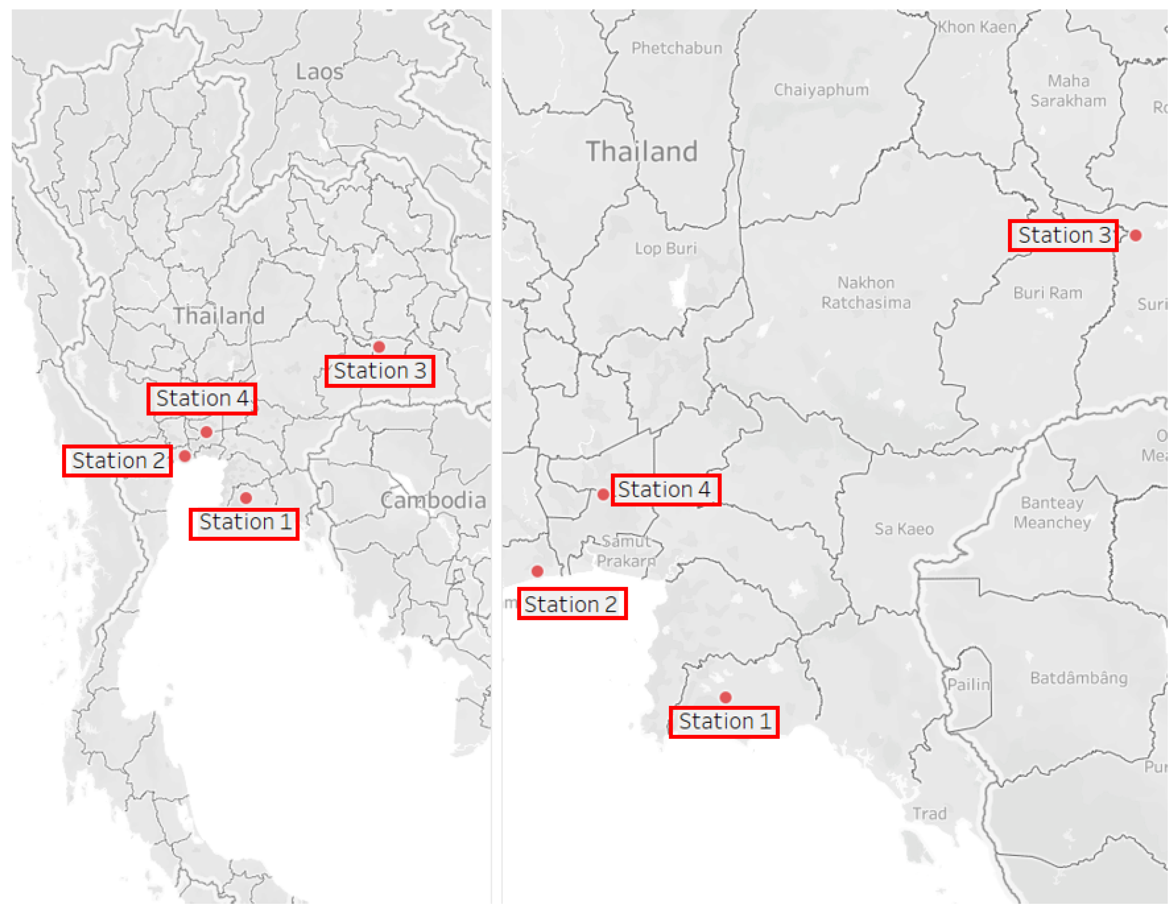
With an exploratory observation, more recent data typically contained less missing values or extremely incorrect values. Stations with overabundant missing values were initially eliminated. Among the remaining data, we removed extreme anomalies and initially imputed missing values with a simple interpolation function. To properly train and test the anomaly detection and data filling methods as our case studies, we selected 2-year data from particular 4 stations as representations of contrasting behaviors. Various locations with different associated basin were selected in order to verify a flexibility and a generalization of our proposed framework. Specifically, the same overall framework was applied to all data from these 4 stations while parameters corresponding to internal models were separately fine-tuned. Descriptions of these selected stations are summarized in
Table 1 while their locations are depicted in
Figure 5.
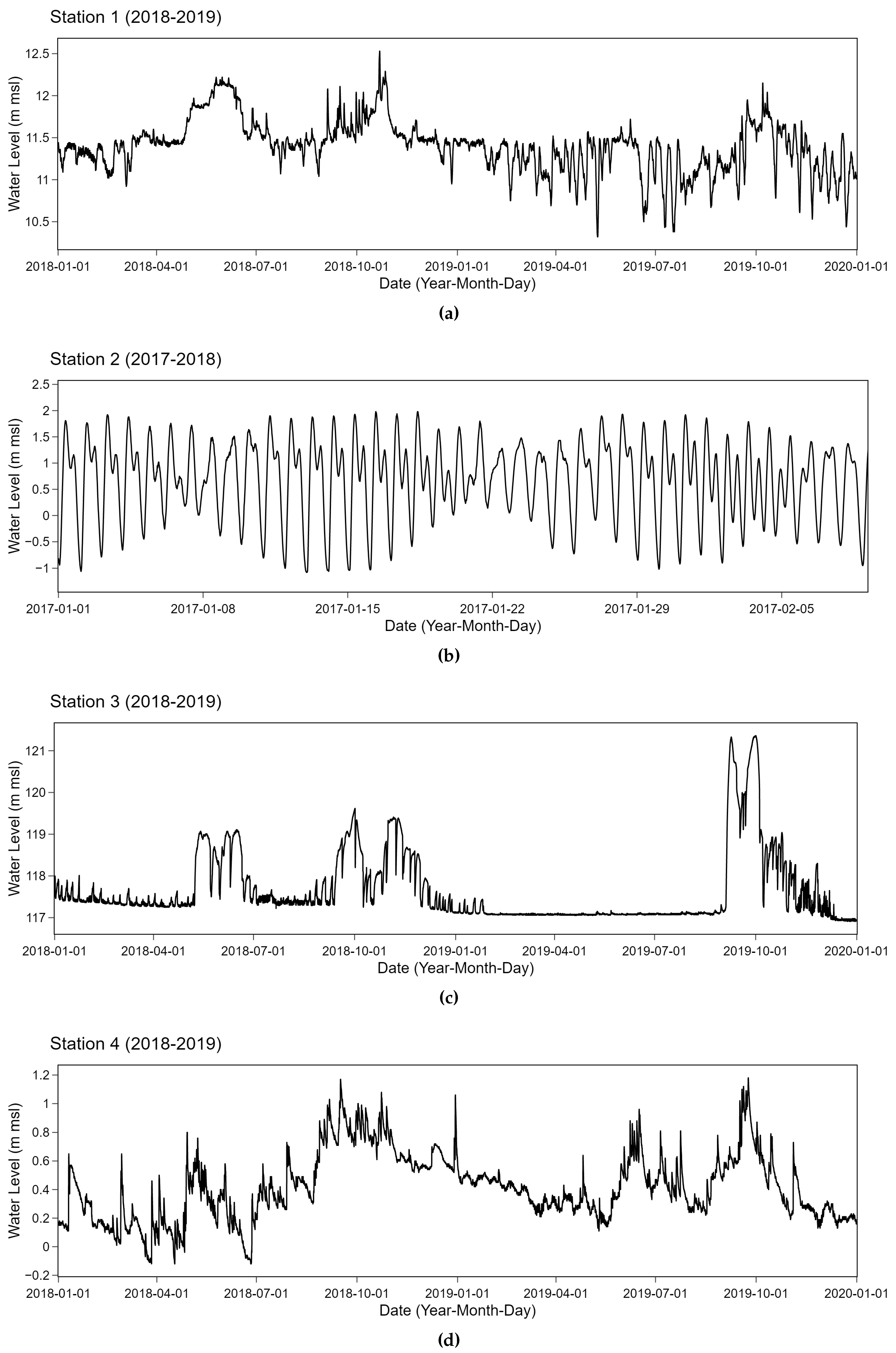
Two consecutive years of relatively complete data with very few missing values of no more than 5% corresponding to selected stations were collected from the original data. These retrieved time series of all 4 stations are depicted in
Figure 6. Time series data from 2017 and 2018 were retrieved for station 2 while other stations relied on 2018 and 2019 data. These time series from specifically selected stations tend to have different behaviors. Strong periodic patterns due to external factors are observed in station 2 which is located near the mouth of the Chao Phraya River connecting to the ocean. A tide effect potentially plays an important role in an observed periodicity. On the contrary, station 3 which is located at a weir has relatively stable characteristics with small changes while abrupt spikes occur at particular points. Additionally, time series data obtained from station 1 and station 4 fluctuate around the mean with different swing behaviors. These inland stations tend to be less influenced by a coastal effect than the other two. More fluctuations are observed in station 4 with several upward and downward trends. These time series having different patterns were collected from telemetry stations. Types of anomalies in the water level data are naturally common. Highly unexpected outliers are rarely noticed. Anomalies types as classified in [
40] in these data include constant offsets with sudden shifts. Clusters of spikes and small sudden spikes can also be observed.
In order to verify the performance of our proposed methods, we held out part of the whole data for evaluating purposes. In particular, the first-year data was used for training while the testing step was performed on the second-year data. As these datasets were collected from sensors without any annotation, annotated labels were required. In order to evaluate the proposed methods, we intentionally removed data points which were hold as the gold standard in our test sets. We separately constructed the test sets for anomaly detection and data filling methods. In these test sets, artificially-created labels were constructed to represent types of anomalies found in our water level data.
3.1.1. Test Data Generation for Anomaly Detection
In order to generate a test data for evaluating anomaly detection methods, 10% of the pre-processed data was converted to anomalies. We initially randomized an integer
A from a range of 2000 to 4000. Then,
A was used as an input for Dirichlet distribution to compute a probability vector
B of length
A that sums to 1. The vector
B was used in Equation (
4) to calculate
K, the length of all intervals of anomalous data where the length of data
l was given.
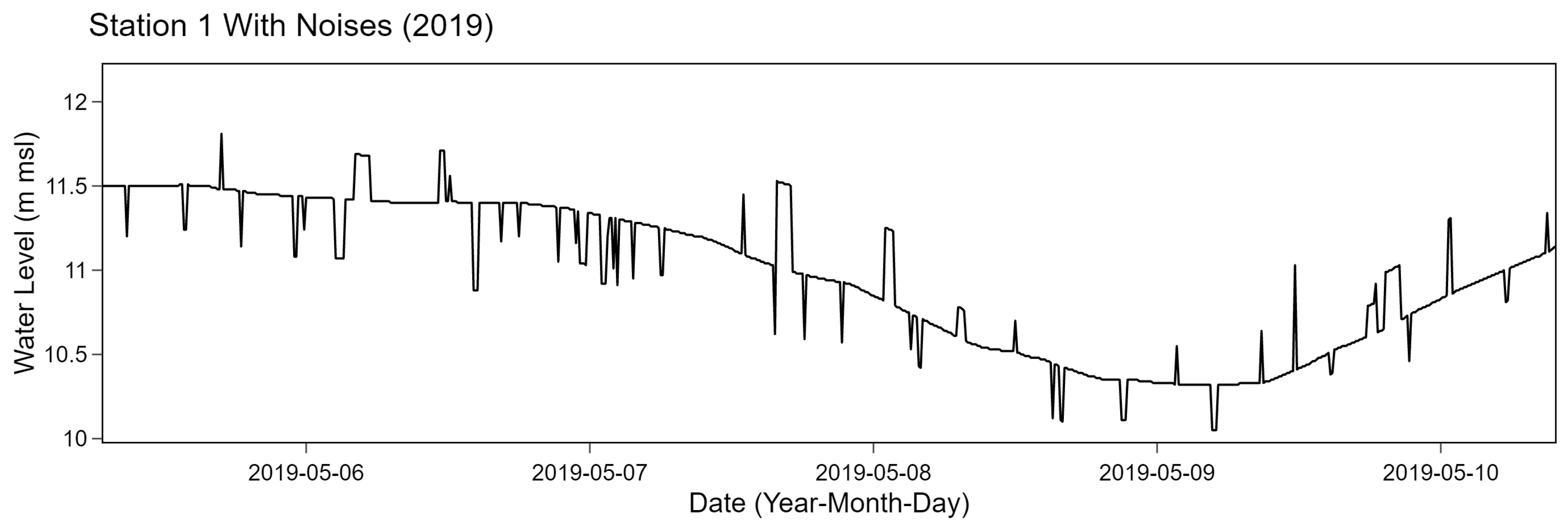
Positions of anomalous data intervals with lengths obtained from
K were randomly selected on the time series data without any overlapping. After specifying the positions of all intervals, noises were added to existing values in the intervals. Noises were selected from the highest value from Gaussian random number generators. Particularly, the Gaussian distribution was implemented with
of 0.2 for station 1, 3, and 4 while
of 0.5 was used for station 2. We specified parameters
to mimic the original data based on a manual observation. An example of result corresponding to station 1 after adding noises is shown in
Figure 7.
3.1.2. Test Data Generation for Data Filling
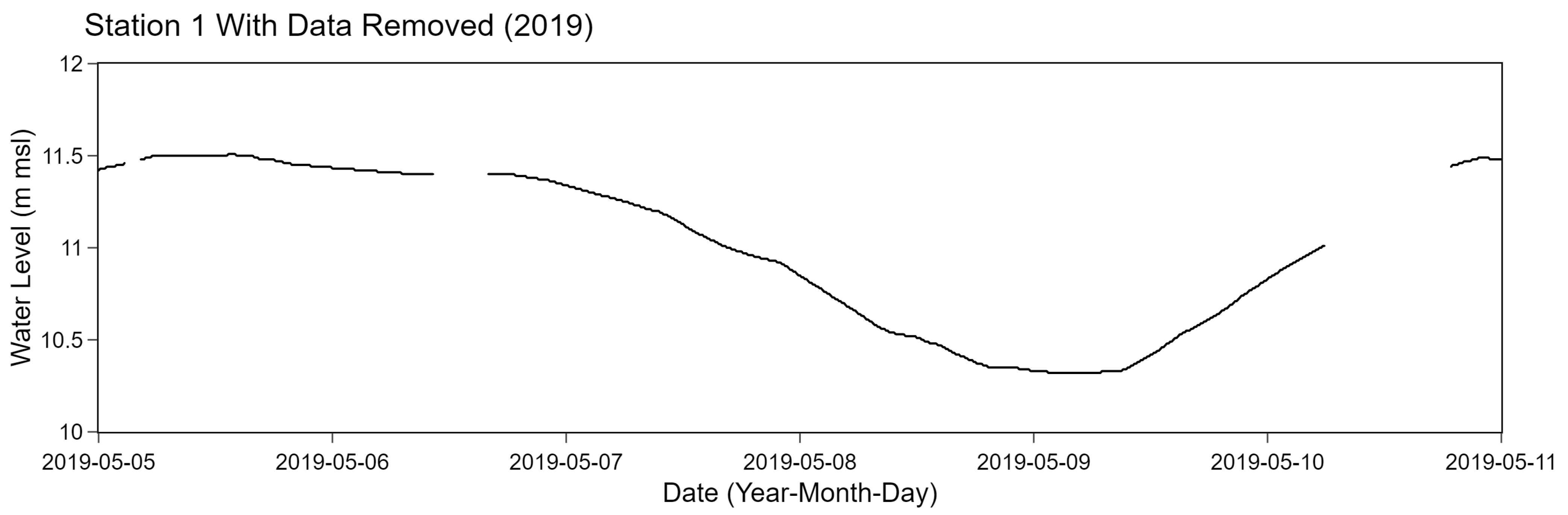
We generated a separate test data for evaluating data filling methods based on 10% of the whole data. A similar approach to generate the test data as discussed in
Section 3.1.1 was also performed. Particularly, the Dirichlet distribution was also applied to compute
K, a list of interval lengths, with a randomized integer
A. Instead of adding noises to the original data, selected points were completely removed. An example of results of station 1 after removing selected data points is shown in
Figure 8.
3.2. Parameters and Training Configurations
Each time series data typically contains different patterns. In order for the proposed methods to work well with various data, associated parameters need to be adjusted accordingly. In particular, involved parameters were thoroughly explored in this work in order to fine-tune for appropriate values. For anomaly detection parameters,
and
were extensively fine-tuned for both median with fixed threshold and MAD methods. These parameters were experimented until superior performance of the proposed method was achieved. Additionally, we modified the original MAD method to include
criteria. Regarding data filling parameters,
k and
s were examined in the spline method while bidirectional LSTM explored
and
parameters. After fine-tuning, all final experimented parameters in the anomaly detection and data filling methods are shown in
Table 2.
In order to properly train LSTM models, all the data were divided into 80% training and 20% validating. Training and validation data were normalized using a min–max scaler. The mean absolute error (MAE) was used as the loss function with ADAM optimizer. A number of epochs, a batch size, min delta, and patience parameters were set to 200, 128, 0.0001, and 20, respectively. In the training step, GeForce GTX 1080 GPU was used in this work.
3.3. Evaluation Metrics
Two common evaluation metrics were utilized in this work. Specifically, F1-score, a harmonic mean of precision and recall, was employed for assessing the anomaly detection performance. The root mean square error (RMSE) comparing between predicted values and the ground truth was used to evaluate the data filling methods.
4. Results and Discussions
The anomaly detection methods with fine-tuned parameters as listed in
Table 2 were evaluated using F1-score, as depicted in
Table 3. Prior to obtain selected parameters, the fine-tuning step was performed. As an example, we further provided sensitivity of F1-score obtained from MAD method of station 1 as shown in
Table 4. Specifically, the
and
were varied while holding another parameter fixed at specified value. Varying parameters utilized in these methods resulted in slight inferior F1-score compared to 0.9944 F1-score corresponding to the selected parameters.
A desirable performance with high F1-score was achieved as reported in
Table 3. Our proposed method is able to estimate so flexible predictive interval that changes in the data are well-captured. Comparing between anomaly detection methods, an average F1-score of the median with fixed threshold was relatively higher than the MAD method. In particular, both methods provided superior performances on all stations except station 2. Considering only station 2 data, the median with fixed threshold method gave 0.8823 F1-score which is higher than 0.7804 F1-score of MAD.
Distinct behaviors of station 2 mostly due to tidal effects can be clearly observed as shown in
Figure 6. Due to the periodicity of the water level data of station 2, we observed that
have to be small enough to capture abrupt and frequent changes in the data. Utilizing large windows potentially relies on many irrelevant observations. As a result, inaccurate estimations due to abrupt changing trends resulting from these observations are observed. We identified the appropriate size of sliding window based on the exhaustive search. The
was on the range of 25 to 55 depending on their variations and time frames. After fine-tuning,
of 25 and 19 for median with fixed threshold and MAD were obtained for station 2. They were relatively smaller than those of other stations. The
effect was less obvious in the MAD method as selected parameters were less deviated among stations. The
was on the range of 0.05 to 3.5 depending on a strong variation at each data point.
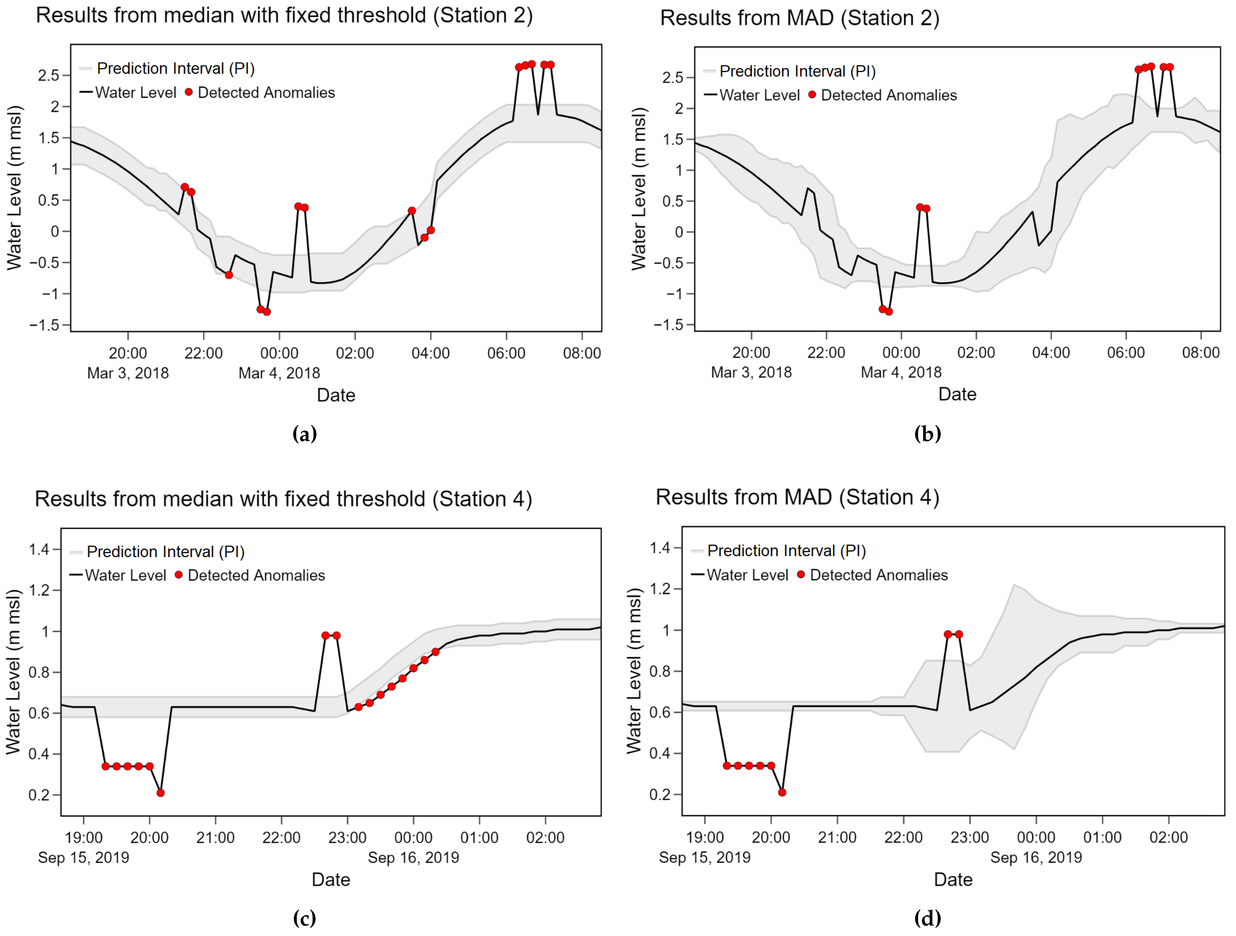
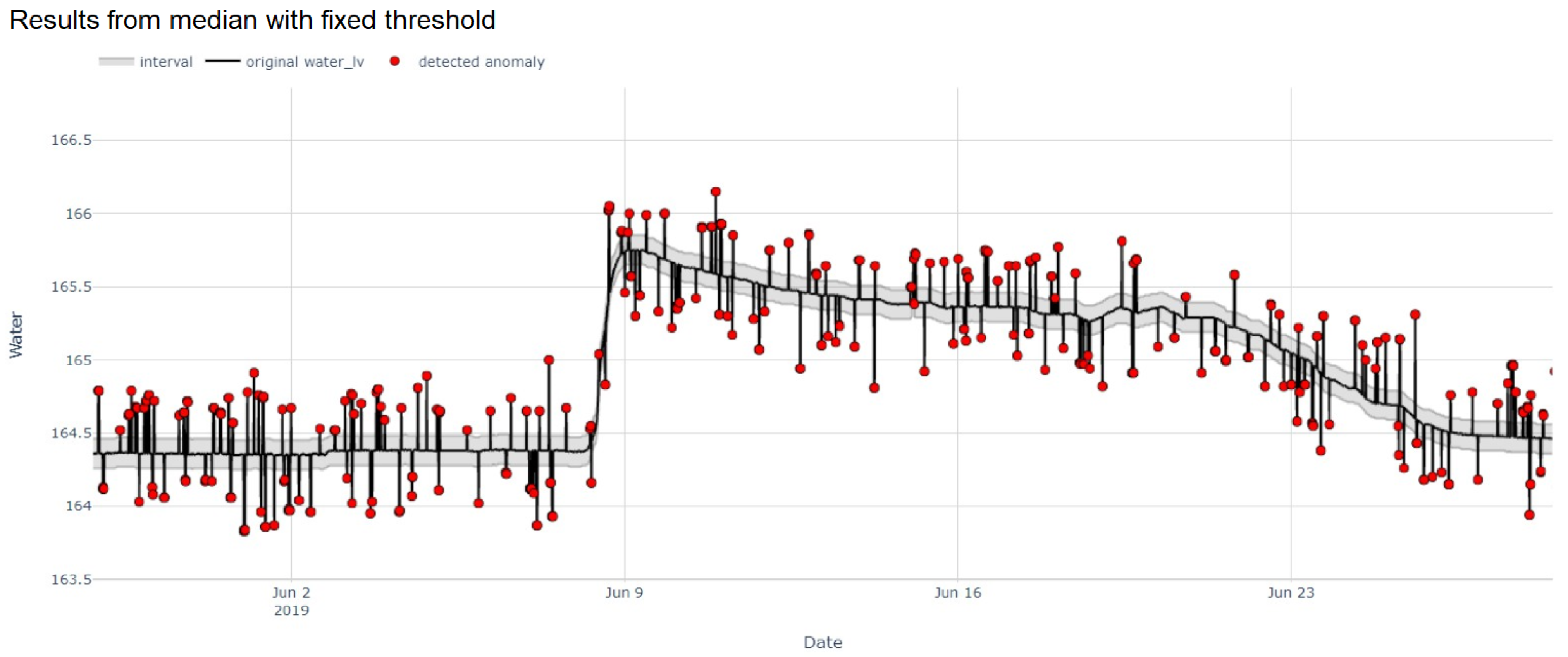
With the current experiment settings, anomalies in some cases were incorrectly identified as normal points in MAD method as shown in the second plot (b) of
Figure 9. The median with fixed threshold method was less affected to such situation as shown in the first plot (a) of
Figure 9. The prediction interval (PI) was calculated from upper and lower values for the median with fixed threshold method while it relied on the Z value for the MAD method, respectively. Based on our observation, the fixed threshold yields more stable PI which is more suitable for data with abrupt and frequent changes like station 2. However, in some situations, as shown in plots (c) and (d) of
Figure 9, the MAD method was able to follow changes in water level better than the median with fixed threshold method. The prediction interval of the MAD method was expandable while the interval of the median with fixed threshold was constantly fixed. Another disadvantage of the fixed threshold can be observed from plot (c) of
Figure 9 where several adjacent points were incorrectly detected as anomalies. When one point is incorrectly classified, subsequent points are likely to follow the same pattern.
Regarding tidal effects, recurrent upward and downward trends are noticeable in station 2 data while infrequent changes with some peaks can be observed in non-cyclical data patterns. According to our observation from the experiments, the tidal effects yielded frequent changes with similar magnitudes in the data. The method with a constant threshold resulting in a fixed prediction interval consequently performed better in the data with tidal effects. On the other hand, the adaptive threshold method like MAD is more capable of dealing with infrequent and unexpected changes.
We further applied our proposed methods with additional data containing infrequent and anomalous step changes to verify their capability. The median with fixed threshold and MAD yielded 0.975 and 0.9693 F1-score as depicted in
Figure 10. With respect to false detection rates, the median with fixed threshold yielded 0.2744 false positive rate (FPR) and 2.4923 false negative rate (FNR) while 0.3904 FPR and 2.5889 FNR were retrieved from MAD. Our proposed methods performed reasonably well even with some abrupt change points commonly found in water level data.
Due to the data imputation perspective, RMSE was employed to evaluate the performance of 3 methods as shown in
Table 5. Considering all stations, the bidirectional LSTM model provided the best performance with 0.0291 average RMSE. However, this method actually performed worse than other methods on most stations except station 2. On the other hand, the spline method yielded desirable performance among station 1, 3, and 4 with 0.0038 RMSE while the linear interpolation yielded 0.004 RMSE.
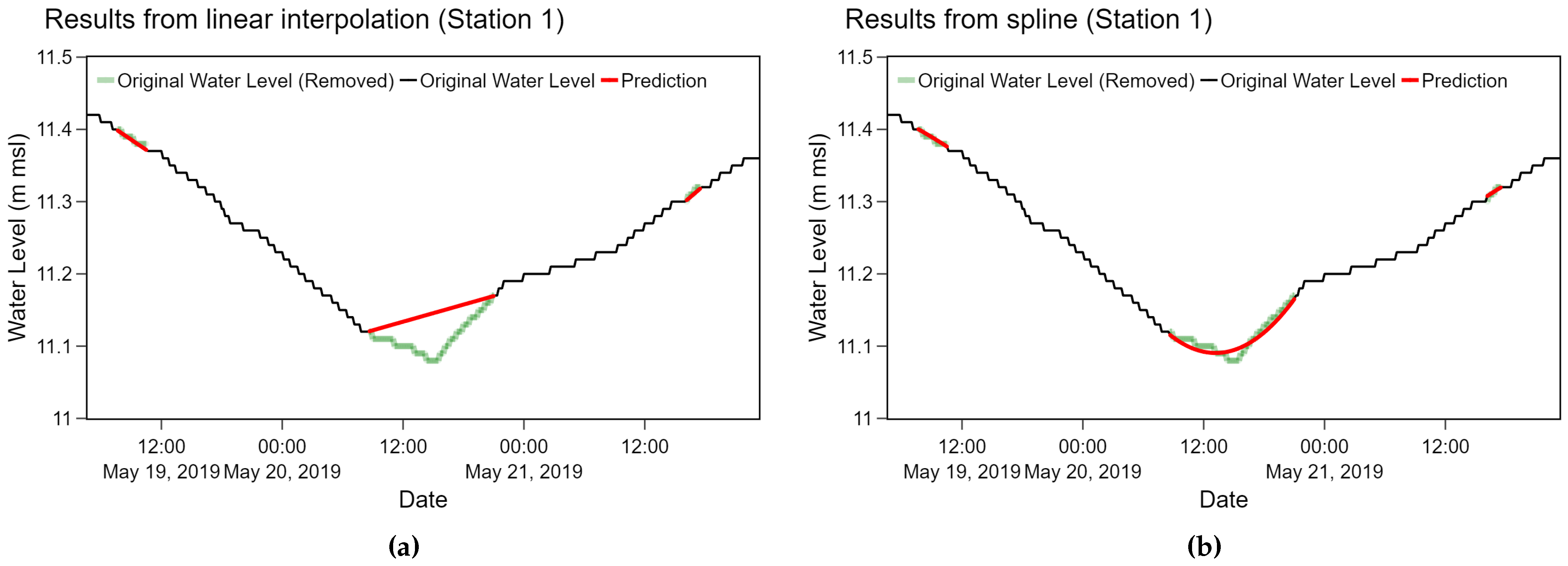
According to both overall average and the average among 3 stations, the spline and the linear interpolation method performed equally well. We observed that results from the spline method were relatively smoother than the linear interpolation as depicted in
Figure 11 where both methods were applied on station 1 data. Even though the spline method is likely to yield a slight better performance at substituting water level data, fine-tuning for appropriate parameters is more time-consuming.
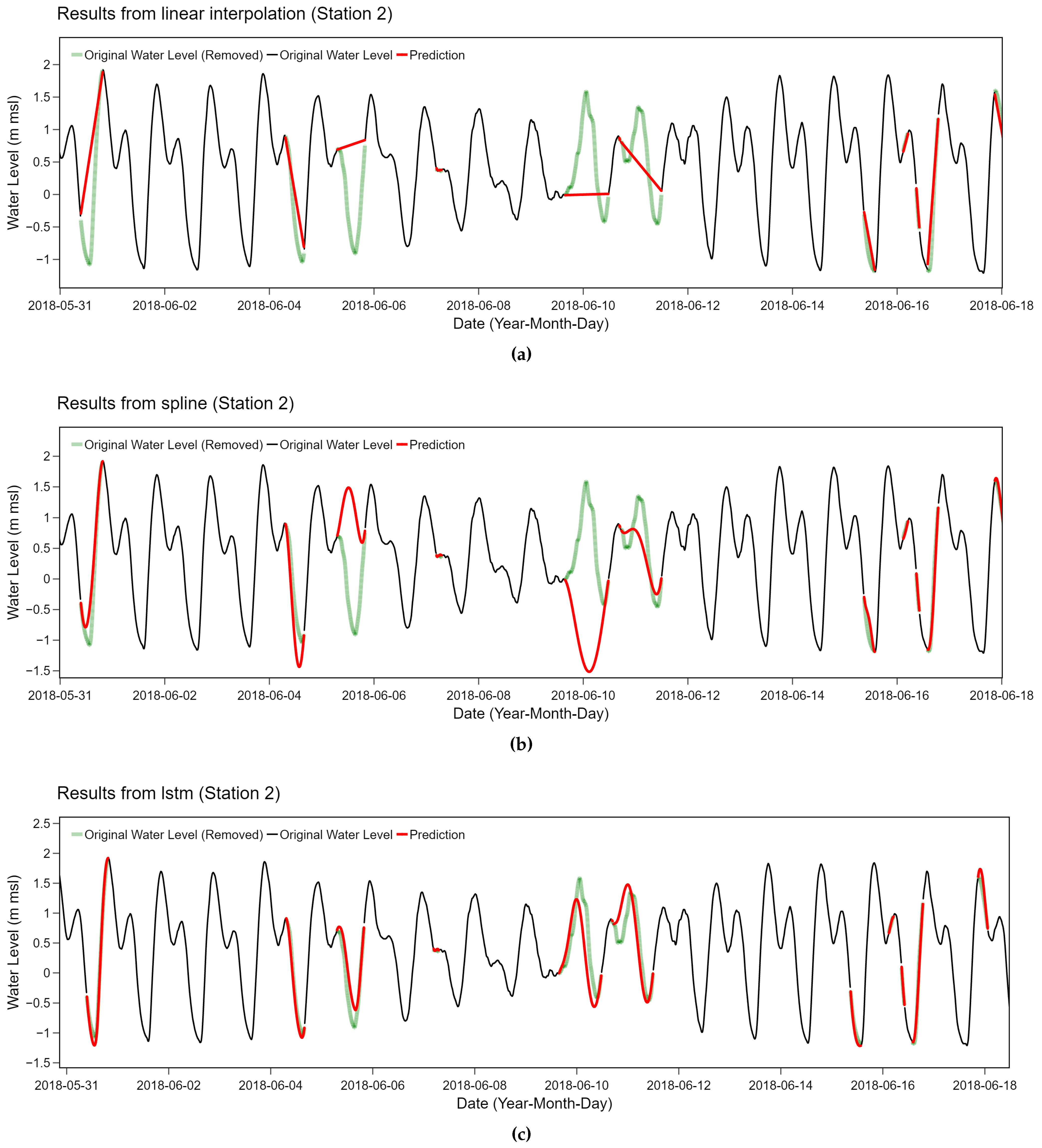
We performed a further analysis on the specific case of station 2. Periodic behaviors of water level at station 2 can be captured with LSTM-based method while the other two methods failed considerably. The utilized bidirectional LSTM model was trained on the input sequence and its reversed copy which preserved both past and future information of a specific time frame. With this advantage, the bidirectional LSTM model is able to understand the context better which is suitable for relatively complicated time series with frequent changes with tidal effects like station 2. According to our experiments, the linear relationship and polynomial functions utilized in the spline method were too naive to capture periodic behaviors, as shown in
Figure 12. Due to the strong periodicity with frequent upward and downward changes, several red interpolation lines do not match with the original green line which has previously been removed. Comparing between these figures, both methods tend to behave similarly as they fail at the same particular points of the data. On the contrary, more complicated method like bidirectional LSTM is suitable for this situation as depicted in the bottom plot of
Figure 12.
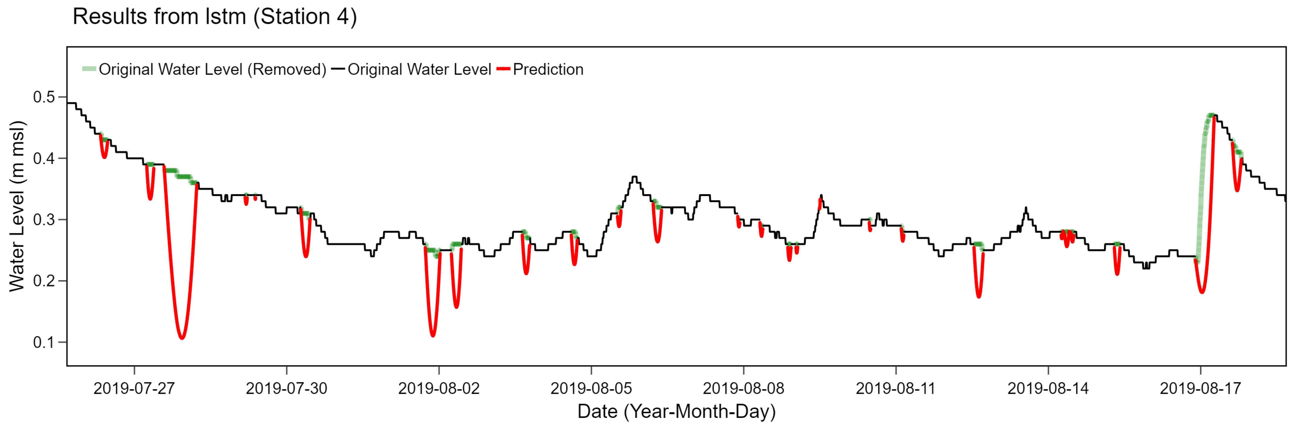
However, the bidirectional LSTM filling method may not provide the best performance in all scenarios. For example, time series of station 4 tend to have smoother patterns with much less seasonality due to tidal effects than station 2. According to our experiment on these data, the bidirectional LSTM method incorrectly estimated too fluctuated values compared to the original time series, as depicted in
Figure 13. The LSTM model was prone to underestimate the ground truth for non-cyclical behaviors without frequent upward and downward trends. The bidirectional LSTM model considered both future and past directions when estimating the final prediction. When one point was incorrectly estimated, adjacent points tended to follow the same tendency. As a result, these errors were further accumulated over time resulting in distinct drop-down miscalculations.
Our current LSTM model was trained with fine-tuned parameters without an over-fitting problem. Particularly, a particular part of the whole training data was intentionally held out for validating. Loss functions on the training and validating parts were observed to avoid the over-fitting phenomenon. The model was carefully trained until loss functions were flattened. We constructed this model based on 1-year time series while training complicated LSTM-based method typically requires large enough dataset to learn patterns. In order to justify the LSTM model performance, an additional experiment by varying a proportion of required training data was conducted. We selected non-cyclical data behaviors like station 1 as an example. Instead of using 80% training data, we reduced this number to 70% and 60% prior to repeating the same experiment for training the bidirectional LSTM model. These models were evaluated and compared with 0.0052 RMSE of current settings as previously reported in
Table 5. According to our additional experiment, 0.0187 and 0.0206 RMSE were achieved from the LSTM models using 70% and 60% training data, respectively. The higher number of training data tends to reduce the model error considerably. Retrieving additional data potentially enhances the performance of our present LSTM model.
To sum up, both statistical-based anomaly detection methods are easy to implement, fast, and require light computation efforts. They tend to perform equally well in most situations. Regarding data imputation, the linear and spline interpolation work well with non-cyclical time series patterns while the bidirectional LSTM method is able to capture periodic behaviors. With the desirable performance as observed in our case studies, applying the proposed methods in an on-line framework for a real-time detection is promising with a slight modification. Particularly, the proposed real-time quality control framework for hydrological data consists of the anomaly detection part which screen out outliers from the data. The imputation method is further applied on detected data to substitute anomalies with appropriate values. Even though this study conducted experiments on the water level data only, the general proposed framework is intentionally designed to be applicable with other hydrological time series data. Additional steps of fine-tuning parameters for other data distributions or different data types are required.
A combination of methods and an application of the models distinguish our work from others. Our main contribution is combining both statistical-based anomaly detection methods under the prediction interval framework with a sliding window technique while implementing machine learning data imputation approaches as an overall system. Compared to previous work [
35] with MAD outlier detection and EWMA smoothing, we utilized the similar approach to identify anomalies but we relied on relatively advanced bidirectional LSTM data filling method. Several works focused solely on the anomaly detection or the data imputation task while we developed the overall system with both components. Our present method allows an adaptive prediction interval, so it can capture anomalies from various data distributions with a small computational time requirement. This technique can be applied for both off-line and on-line detection which is suitable for a data monitoring system. To the best of our knowledge, none of prior works applied a similar framework on a dataset collected in Thailand. Our case studies consisted of time series data collected from several telemetry stations among various locations. We explored diverse data patterns especially the strong periodicity which required a specific treatment. We performed thorough experiments comparing between multiple data behaviors, such as cyclic and non-cyclic (with and without tidal effects), as well as infrequent abrupt changes.
To enhance the proposed quality control framework for time series data, applying machine learning algorithms, such as isolation forest or deep learning algorithms as the anomaly detection method with the sliding window technique is promising. Further integrating seasonality (e.g., wet and dry seasons) and change-point features in the proposed model to represent unexpected spikes commonly found in the water level data are an encouraging enhancement. Another direction of future work includes specifying groups of stations with pre-defined parameters without extensively fine-tuning. This will further improve the efficiency and practicality of the proposed framework. Instead of considering each individual station for the data filling method, a spatial-temporal relationship which relies on nearby stations is compelling. Finally, applying the proposed framework with other hydrological data extends the completeness and the generalizability of this work considerably.


 ,
, 


