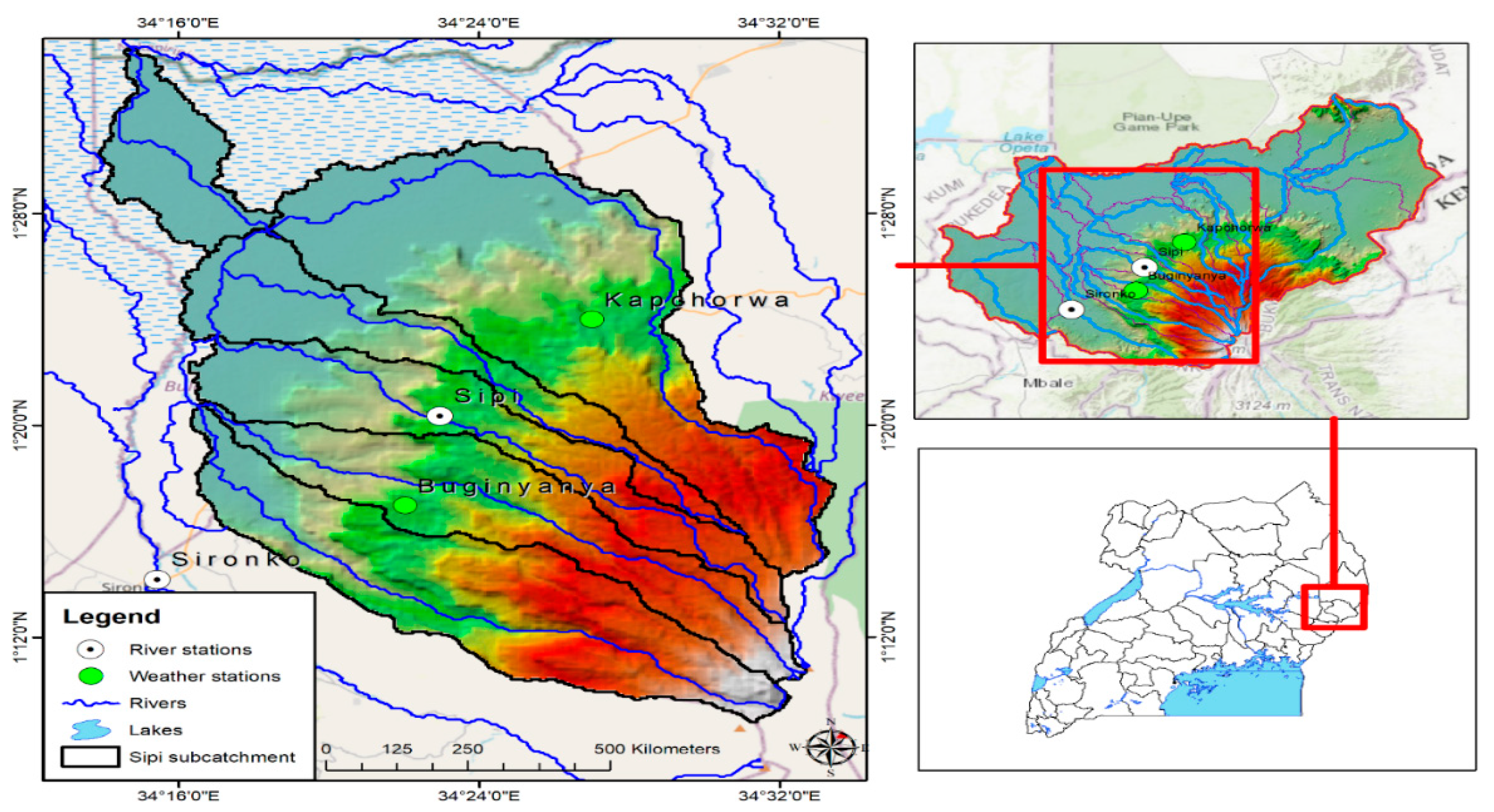
This study was conducted in the River Sipi sub-catchment (918 km
2) of the Sironko catchment (3997 km
2) on the slopes of Mt. Elgon in Eastern Uganda (
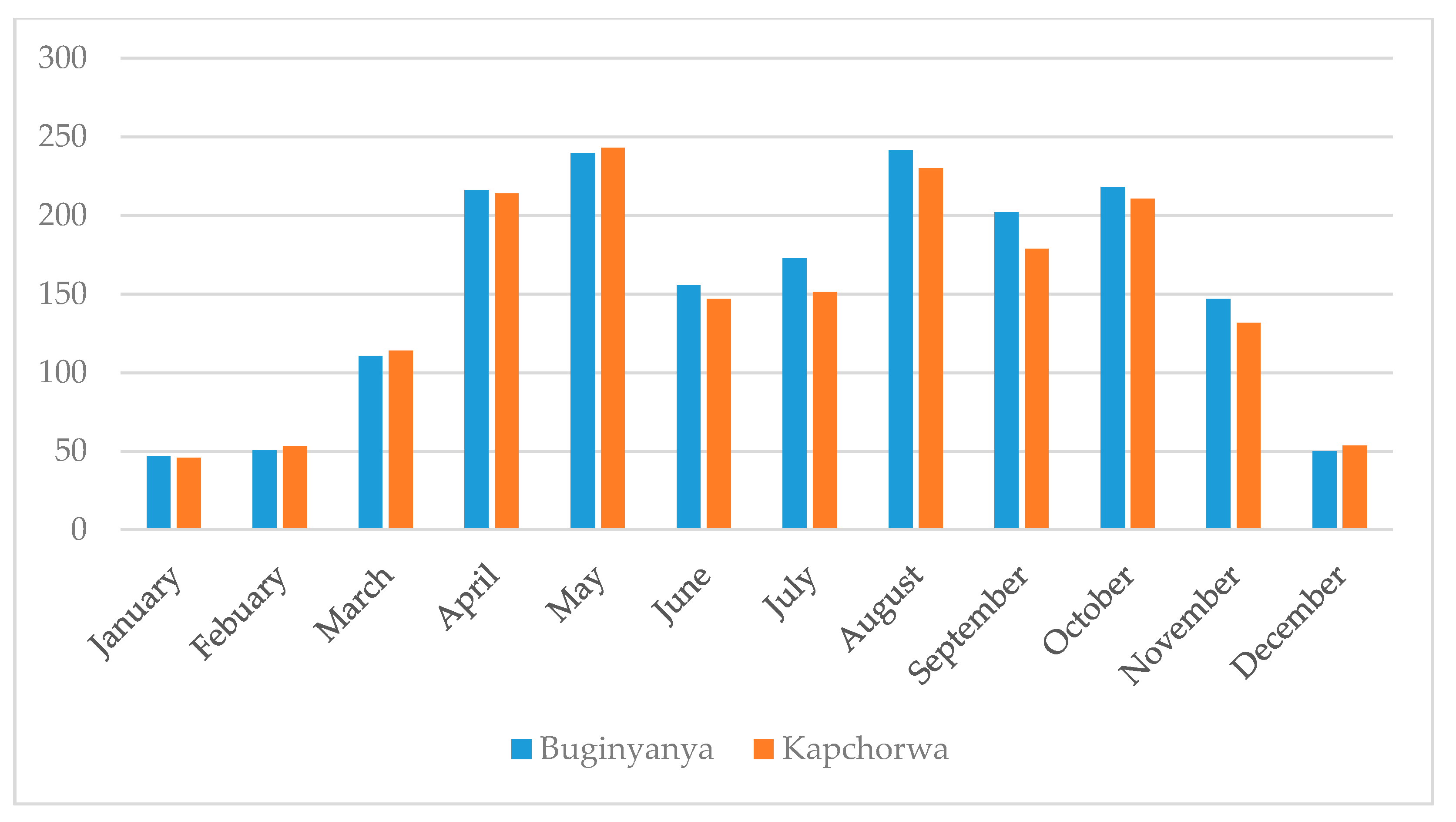
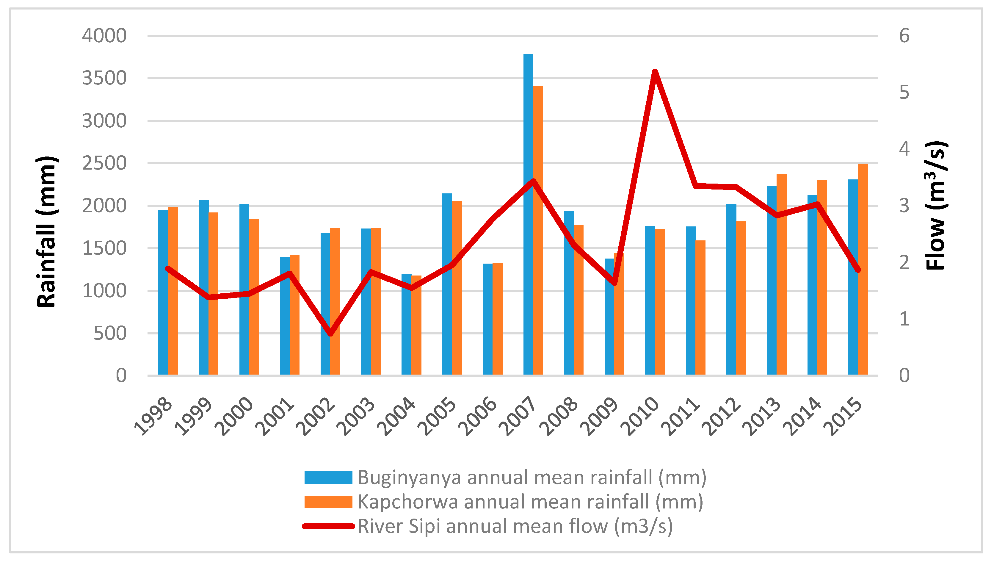
Figure 1). The sub-catchment exhibits a bimodal rainfall characteristic where the first rainfall season takes place from March to May, while the second rainfall season takes place from August to November (
Figure 2). The mean annual rainfall over the sub-catchment for the period 1981–2015 was 1812.3 mm, and the mean temperature was 21.7 °C. Small-scale agriculture is the prominent source of livelihood in the sub-catchment and the main crops grown are maize, beans, sweet potatoes, banana, and coffee. The local communities in the Sipi sub-catchment use the rivers water for small-scale irrigation, domestic and urban water supply, livestock watering, fishing, and recreational activities.
2.2. Data Analysis
The mean, standard deviation (SD), and coefficient of variation (CV) in Equation (1) formed the first analysis for the rainfall, temperature, and river-flow data. These methods have been used by [
9,
11,
18,
26]. The analysis was carried out at the individual stations’ level and over the entire sub-catchment. The rainfall and temperature data for Buginyanya and Kapchorwa were averaged in order to compute the variability over the sub-catchment. The annual, MAM, and ASON seasons were adopted (
Figure 2).
where CV is the coefficient of variation, δ is the standard deviation and μ is the mean of the dataset. When the CV is high, the variability is considered to be high and when the CV is low, the variability is considered low. The rainfall is considered less variable when CV ˂ 20, moderately variable when, 20 ˂ CV ˂ 30, and highly variable when CV > 30 [
11,
27].
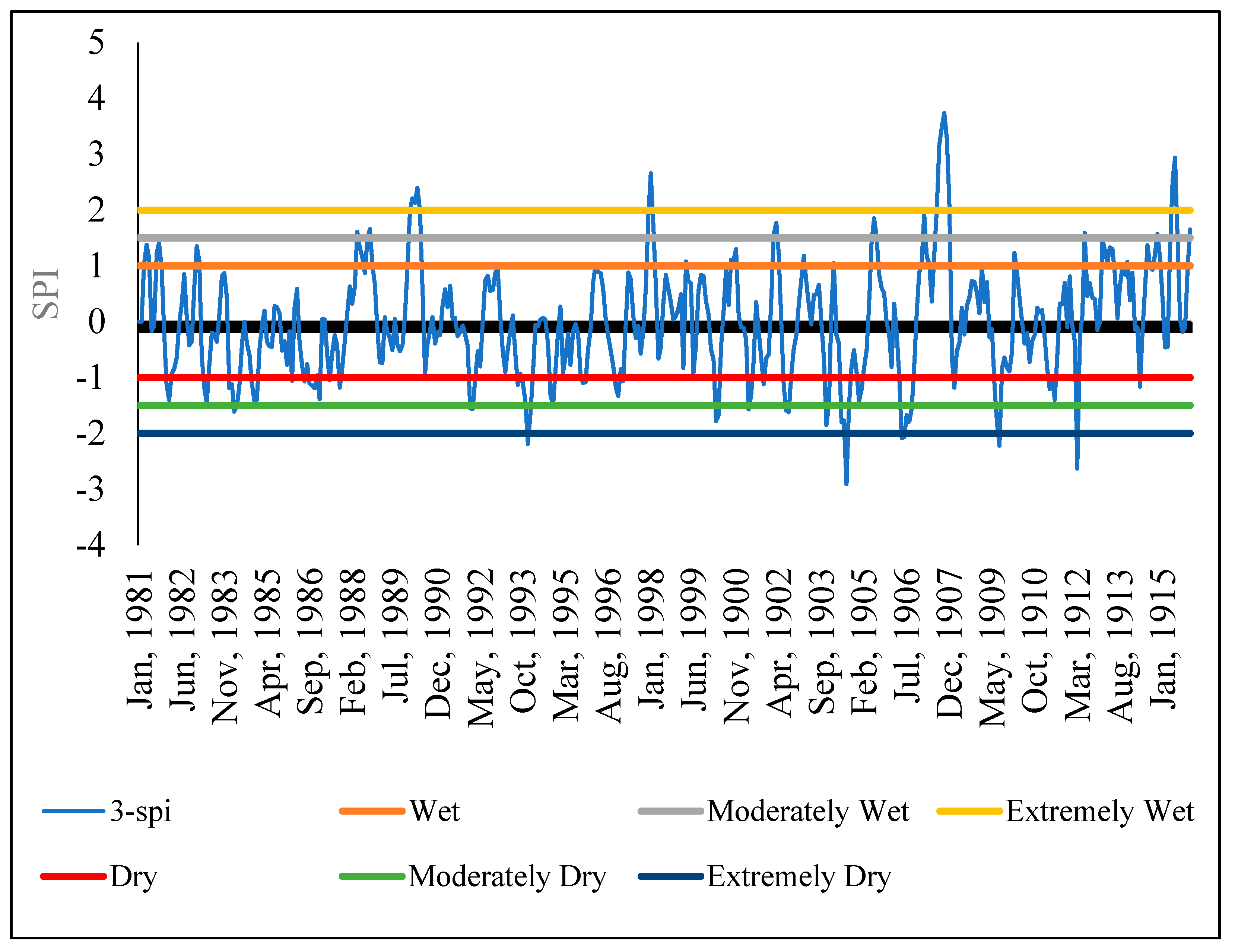
The Standardized Precipitation Index (SPI) formed the second part of the analysis for rainfall data. It was used to determine the sensitivity of the sub-catchment to extremely wet and dry periods. SPI is calculated based on long-term precipitation data for a given location and a specific period. The scale of SPI can start from 1 month, 3 months, 6 months, 9 months, 12 months, 24 months, 36 months, and 48 months). The selection of the SPI scale is determined by the purpose for which it is being calculated. However, irrespective of the scale, SPI gives information on the impacts of wet/dry conditions on water availability for different needs. In this study, the 3-month, 6-month, and 12-month SPIs were calculated using the Meteorological Drought Monitor [
28] method to determine extremely wet and dry periods in the Sipi sub-catchment Equation (2).
where χ is the SPI monthly total precipitation, μ is the SPI long-term mean precipitation, and δ is the standard deviation for the SPI precipitation. SPI measures the deviation in standard units between a dataset and its mean [
29,
30]. This study adopted the classification scheme of Reference [
28] in
Table 2. The (3-month, 6-month, and 12-month) SPIs were selected to identify the relative tendency towards above or below normal seasonal and annual precipitation [
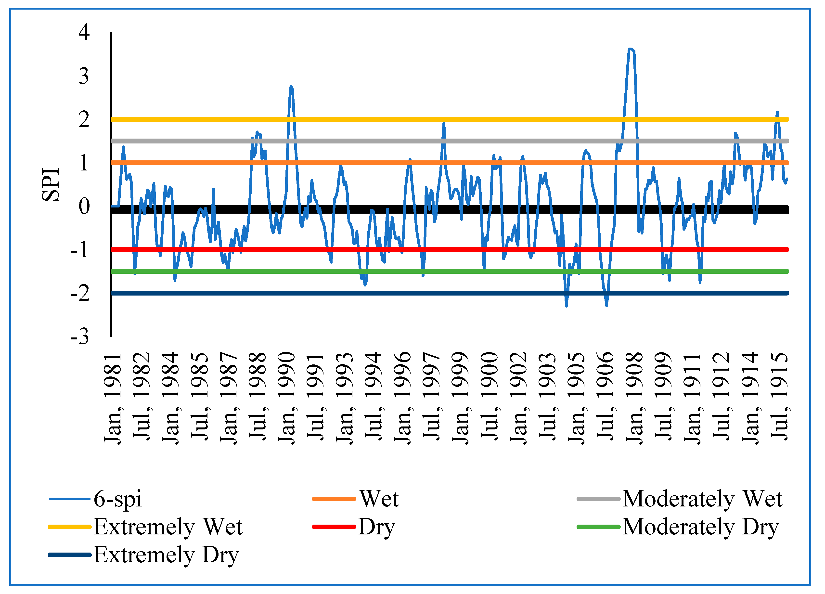
31]. Each SPI scale is a comparison between the specific SPI time scale for the same period recorded in all the other years included in the dataset. A 3-month SPI estimated at the end of September 2010 compares the precipitation total recorded during July, August, and September 2010 and the precipitation total recorded during the same set of months in all years before 2010 in the same dataset. As stated before, a 3-month SPI was selected to represent the seasonal estimations of precipitation and to provide a measure of the short-term moisture conditions. The 6-month and 12-month SPIs, on the other hand, were selected because they reflect the medium- and long-term moisture conditions, respectively. According to [
32,
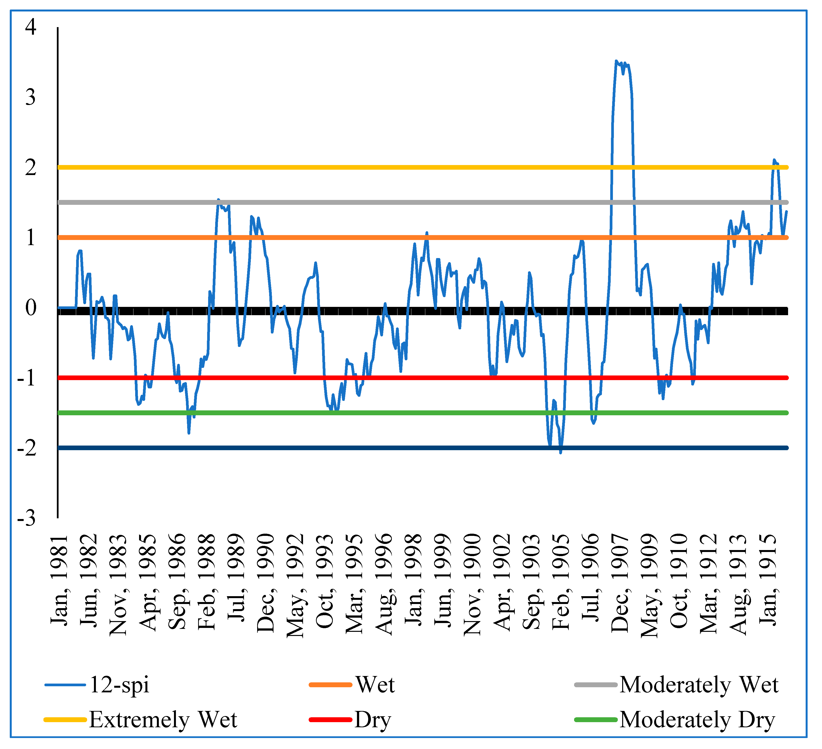
33], information retrieved from the 6-month and 12-month SPIs can be used to capture variability in streamflow regimes and reservoir levels. The 6-month and 12-month SPIs can also provide information about the precipitation fallen during a 6-month and 12-month period [
32]. According to [
31], comparing short-term SPI with medium- and longer-term scale SPIs is vital because a relatively normal or even a wet 3-month period can occur in the middle of a long-term drought, and that, in turn, can be captured only by a long-term SPI.
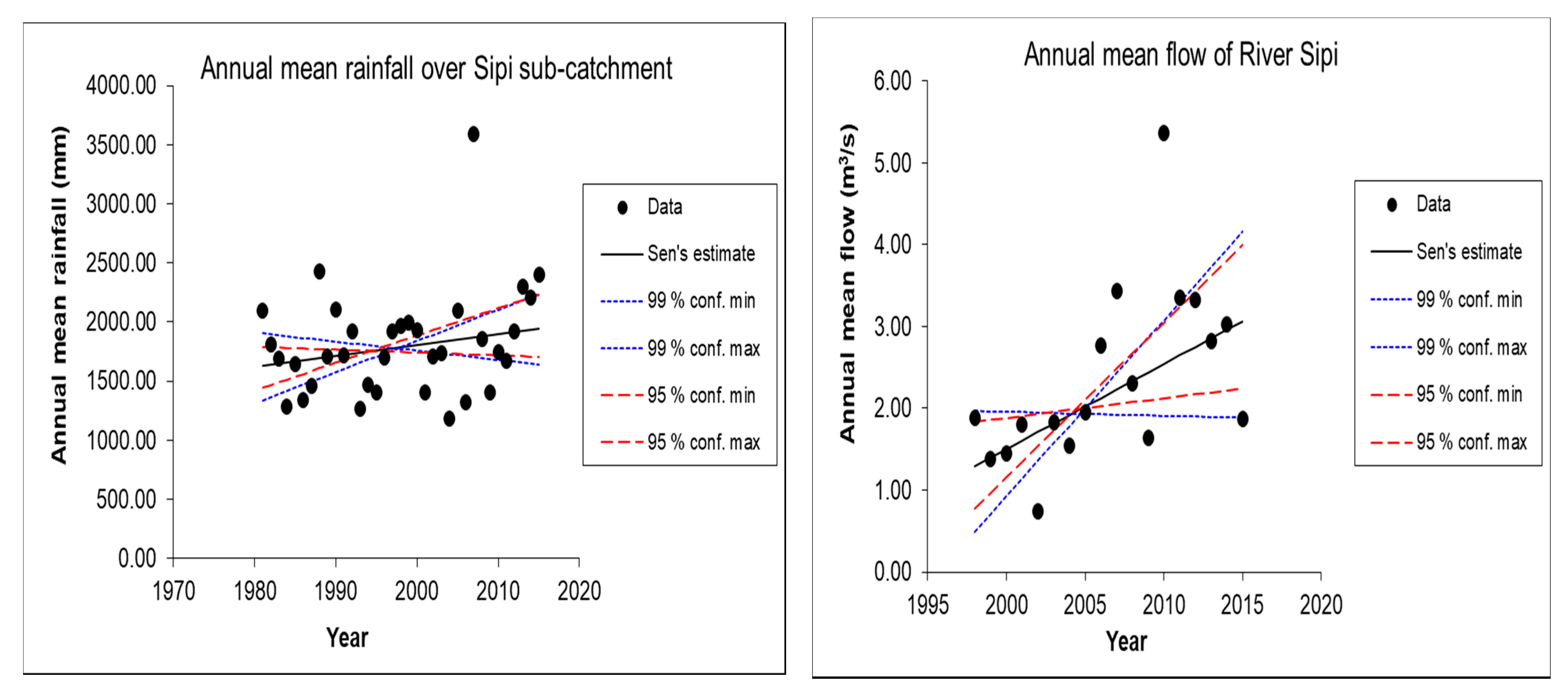
The Mann–Kendall trend analysis and Sen’s slope estimator [
35] formed the last part of the analysis. The Mann–Kendall (MK) test is a nonparametric test, it was used because it does not require the data to be normally distributed, and is not very sensitive to missing data values [
35]. The test has been used to detect both trends and shifts in climate and hydrological time-series datasets [
36,
37]. The test statistic,
S, is based on the null hypothesis that there is no trend or serial correlation in a set of observations.
S was calculated by using Equations (3)–(5):
where
are
the sequential data values,
n is the length of the dataset, and we have the following:
If n is 9 or less, the absolute value of
S is compared directly with the theoretical distribution of
S derived by Mann–Kendall [
35]. In MAKESENS, the two-tailed test is used for four different significance levels of α: 0.1, 0.05, 0.01, and 0.001 [
35]. At a certain probability level, H
0 is rejected in favor of H
1 if the absolute value of
S equals or exceeds a specified value
Sα/2, where
Sα/2 is the smallest
S which has the probability less than α/2 to appear in case of no trend [
35]. A positive/(negative) value of
S indicates an upward/(downward) trend. The significance level of 0.001 means that there is a 0.1% probability that the values
xi is from a random distribution and with that probability we make a mistake when rejecting H
0 of no trend. Thus, the significance level of 0.001 means that the existence of a monotonic trend is very probable. In the same way, the significance level of 0.1 means there is a 10% probability that rejecting H
0 is a mistake.
If n is at least 10, the normal approximation test is applied. The validity of the normal approximation reduces for the number of data values close to 10 for several tied values in the time series. The variance of
S is first computed by following Equation (6) which takes into account that ties may be present:
where
m is the number of tied groups, and
is the size of the
ith tied group.
The standardized test statistics,
Z, is computed as from Equation (7):
The presence of a statistically significant trend is confirmed using the
Z value. A positive/(negative) value of Z indicates an upward/(downward) trend. The statistic
Z has a normal distribution. To test for either an upward or downward monotone trend (a two-tailed test) at α level of significance, H
0 is rejected if the absolute value of
Z is greater than
Z1-α/2, where
Z1-α/2 is derived from the standard normal cumulative distribution [
35]. In MAKESENS, the tested significance levels α are 0.001, 0.01, 0.05, and 0.1. For the four tested significance levels, the following symbols are used: *** if trend at α = 0.001 level of significance, ** if trend at α = 0.01 level of significance, * if trend at α = 0.05 level of significance, and + if trend at α = 0.1 level of significance. If the cell is blank, the significance level is greater than 0.1. In this study, trends were reported at (α = 0.001 and α = 0.05) levels of significance.
The Sen’s slope estimator, Q, is a nonparametric method developed by [
38]. Sen’s slope estimated the magnitude of trends in time series data. For N pairs of data, Q is given by Equations (8) and (9):
where Q is the slope between
xi, and
xj at times
ti and
tj for (
I ˂
j). The value of Q is derived from the median slope for N numbers of slope from the following equation:


