3.1. The Seasonal Variability of the Baltic Sea Level Spectra
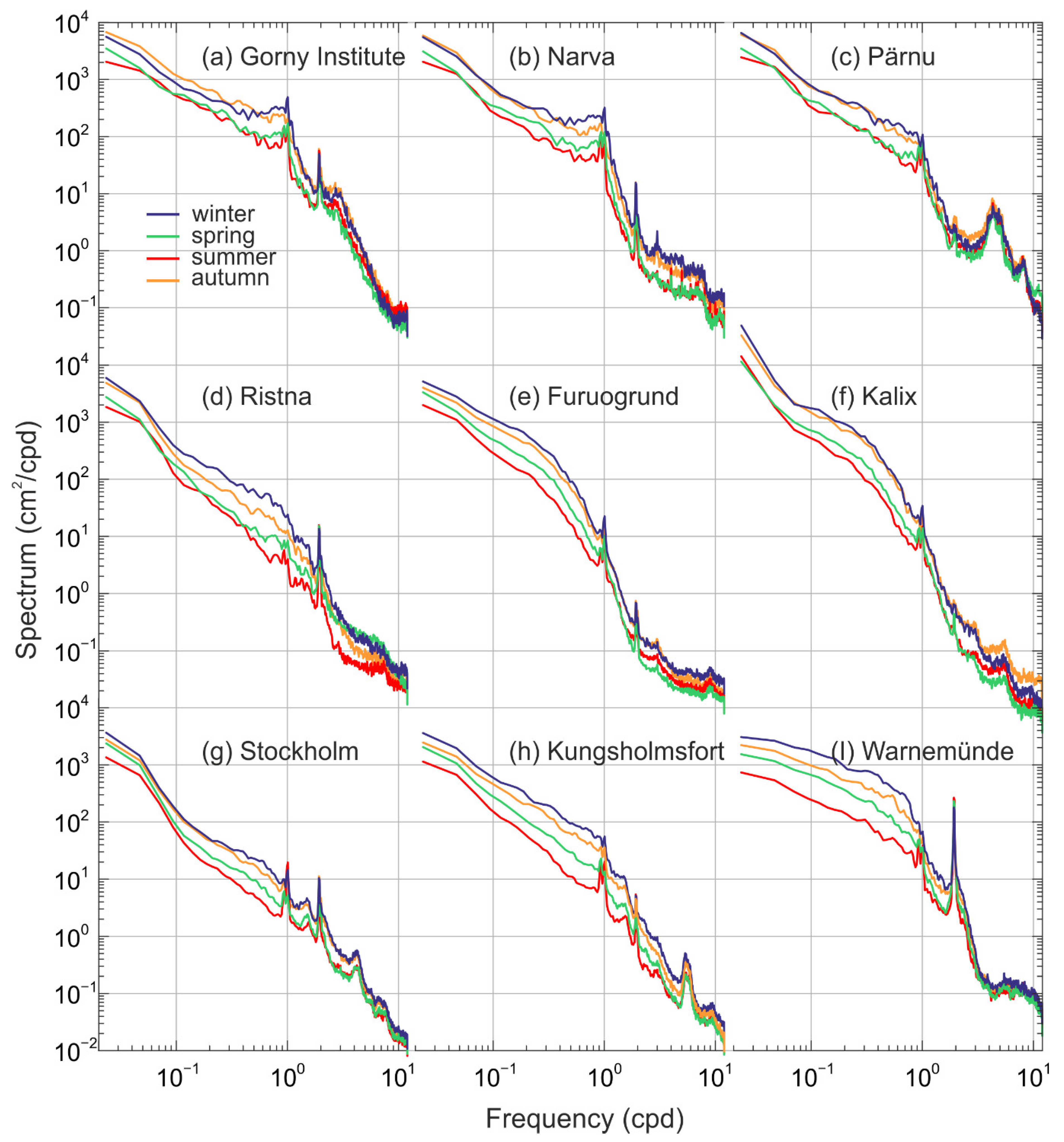
We calculated spectra at nine tide gauges for four seasons (
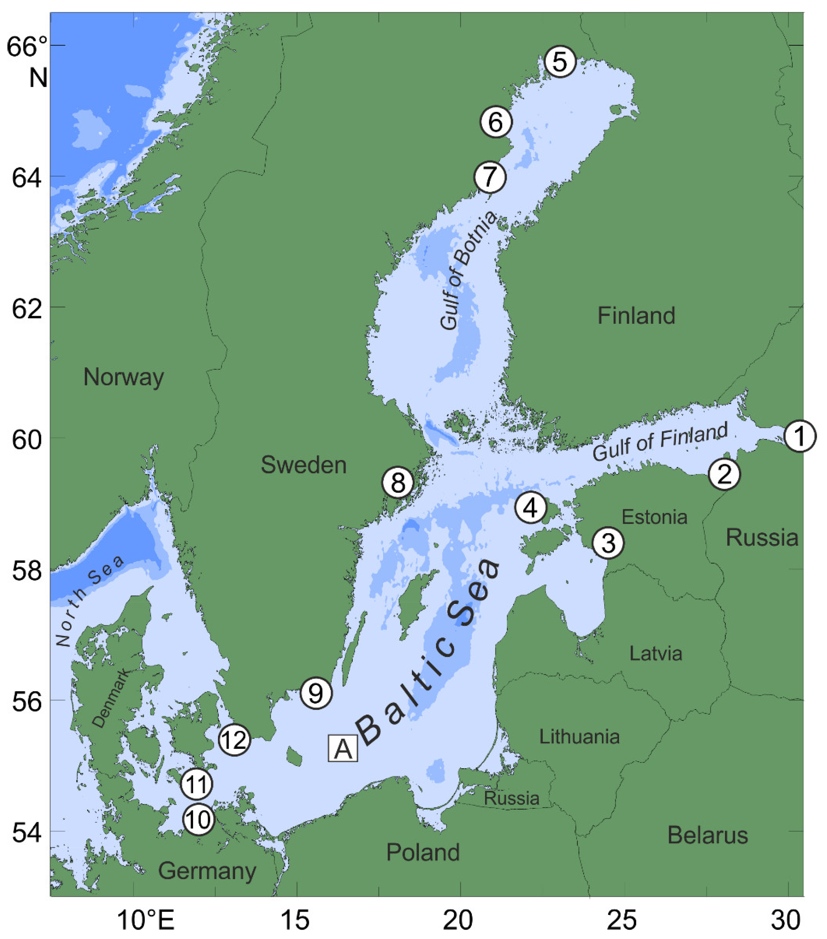
Figure 2): winter (DJF), spring (MAM), summer (JJA), and autumn (SON). The spectra were calculated for each separate 3-month time series and averaged over the full length of the records (31–127 years). There is a significant seasonal change in the spectral density of the continuum spectrum (continuum) in the synoptic frequency range~from 0.03 to 0.5 cpd for all stations. The highest values of spectral density are observed in winter. In spring, the spectral density in this frequency range decreases. It reaches its minimum in summer. Then it increases in autumn again. In spectra at most tide gauges, the maximum spectral density of the continuum is observed in winter, and it is less in autumn. However, in the head of the Gulf of Finland (Gorny Institute and Narva), the Gulf of Riga (Pärnu), and the Gulf of Bothnia (Kalix), the spectral density in winter and autumn does not differ. At the Gorny Institute, the autumn spectrum is even higher than in winter. This is probably due to the location of these tide gauges. The possible influence of the ice cover in the winter months can reduce the variance of the sea level oscillations of wind origin in the head of gulfs. The differences in the summer and spring spectra are negligible at the Gorny Institute, while at the other stations, the difference between the summer and spring spectra is significant.
The difference between the spectra at various seasons decreases with increasing frequency. Therefore, for the Gorny Institute, Pärnu, and Warnemünde, these spectra for four seasons merge. These tide gauges are located at the head of the bays, where the maximum amplitudes of seiches and the maximum of the variance of the mesoscale sea level oscillations in the Baltic Sea are observed [
5]. At the other stations, in general, at the mesoscale, the same spectral pattern is observed as in the synoptic one. However, in the Gulf of Bothnia (Kalix and Furuogrund), the summer spectrum exceeds the spring one. This is possibly caused by the influence of the ice cover. In the spring, it still covers a significant area of the Gulf of Bothnia and thus prevents the formation of sea level oscillations with wind origin.
The spectral peaks with periods of 4, 5, 6, 7, and 8 cpd are observed at the summer spectrum of Narva. These peaks are less in the spectra of other seasons. This confirms the assumption of [
1] that these peaks are radiational tides, and they are caused by the local influence of sea-breeze winds.
In general, the results of the spectral analysis showed a significant seasonal modification of the Baltic sea level spectrum. This seasonal variability is caused by seasonal changes of the driving forces, primarily, of the wind and atmospheric pressure fields and the cyclones trajectories.
3.2. Seasonal Changes of the Sea Level Variance
We calculated the variance of the synoptic
and mesoscale
sea level oscillations for individual months to obtain their seasonal variations.
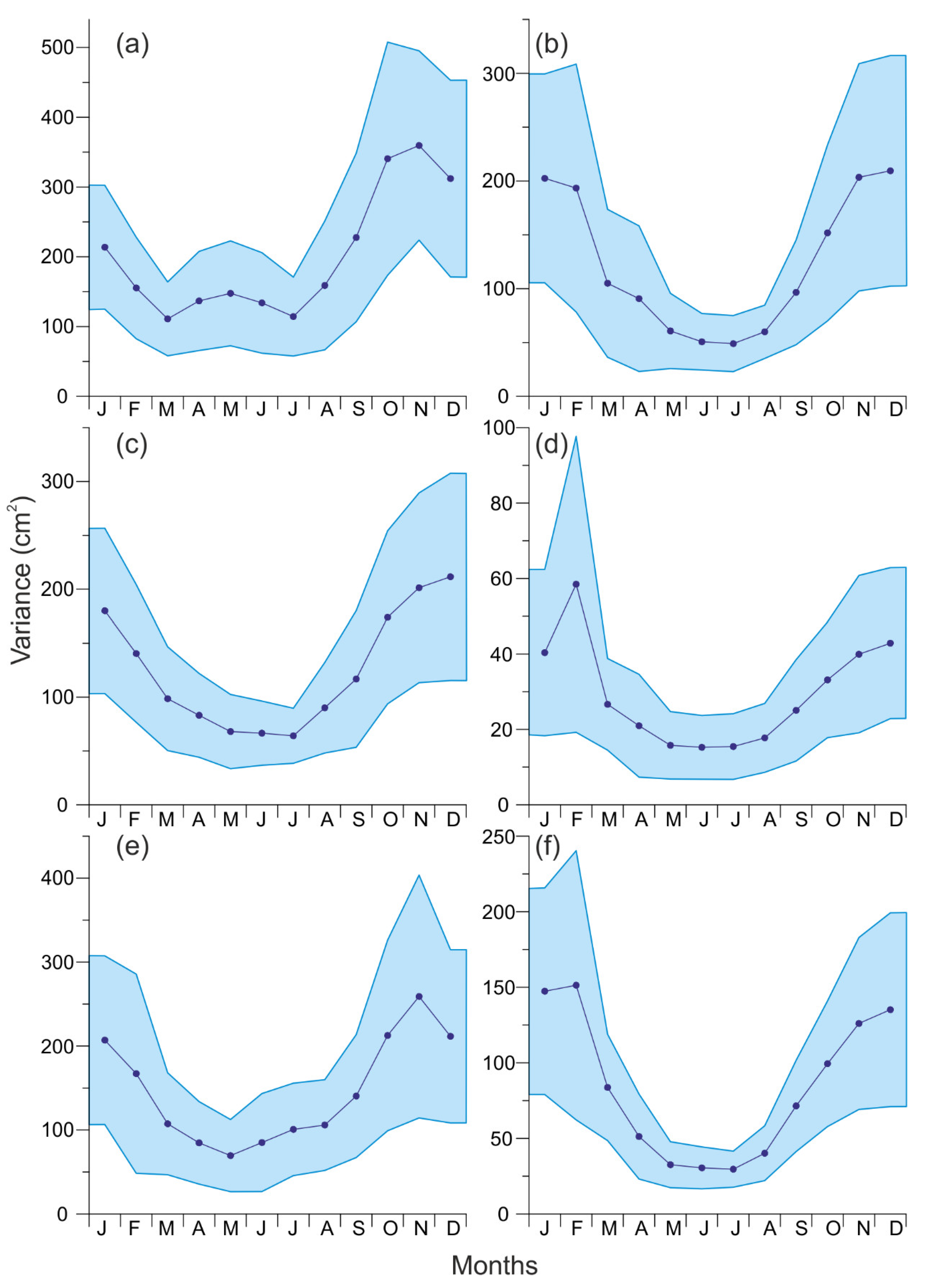
Figure 3 illustrates the results of these estimations for the synoptic scale. All tide gauges are characterized by a seasonal variation with a minimum in the summer and an increase of
in November–December. The variances of
from November to February are 2–3 times higher than in the summer. A small local maximum
is observed at the Gorny Institute in May (
Figure 3a). Probably, this variance maximum is formed under the influence of the Neva River runoff. In the head of the Gulf of Finland (Gorny Institute) and Gulf of Riga (Pärnu), the absolute maximum of
is reached in November. At Narva and Ratan, it is reached in December, and at Stockholm and Kungsholmsfort in February. At the head of the Gulf of Finland,
is 5–10 times greater than in the central part of the sea (Stockholm).
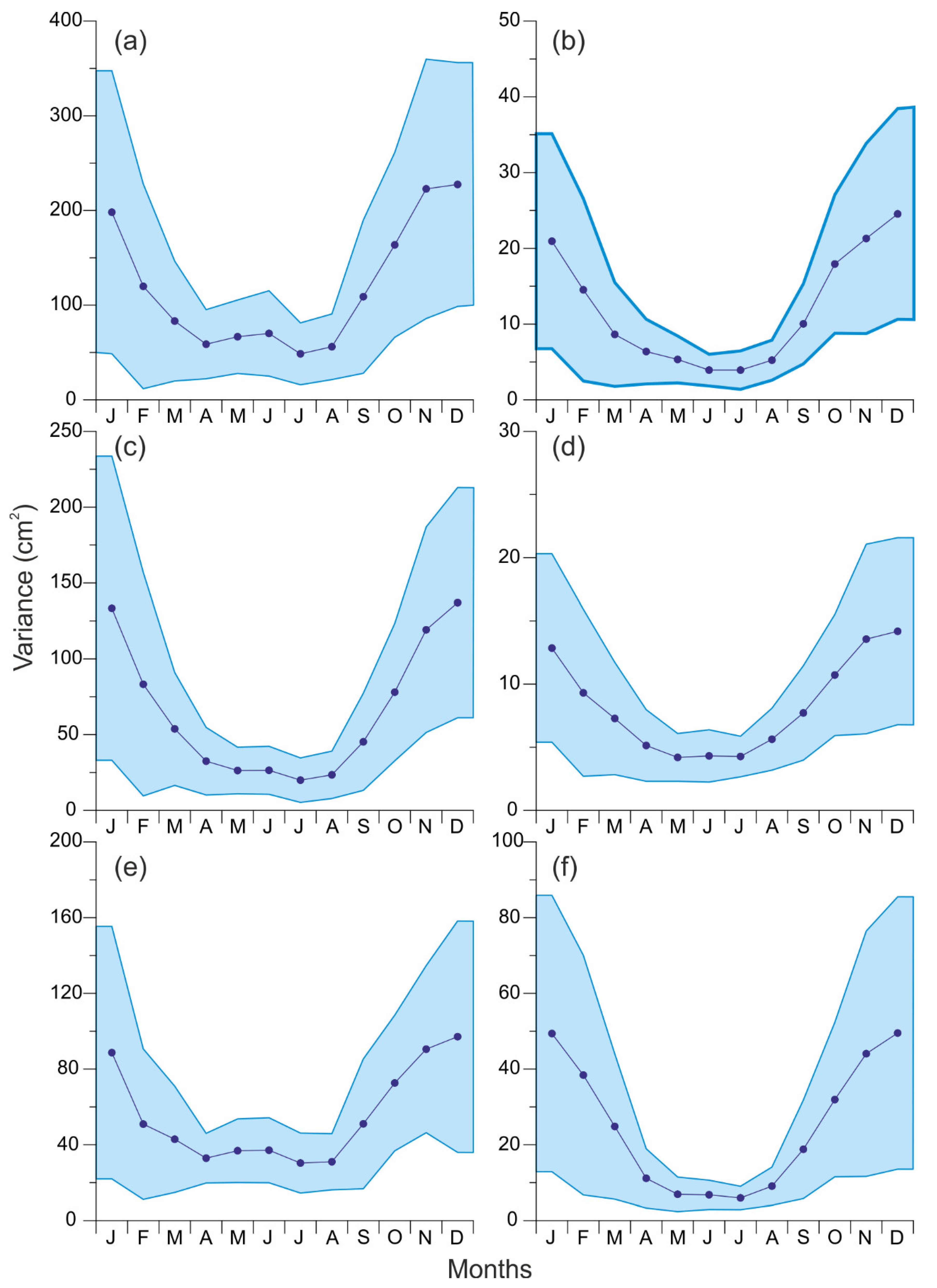
The seasonal variation of
is generally similar to the
seasonal variability: the minimum is in summer, and the maximum happens in December (
Figure 4). However, if for all six stations
increases by about 2–3 times more in the winter than in the summer, then
is 5 times higher in the winter than in the summer. At the Gorny Institute (
Figure 4a), a local maximum of
is again found in May–June. A similar maximum is also observed at Pärnu, Narva, and Stockholm (
Figure 4c–e).
The
and
values were calculated for every month of every year. We estimated the scatter of interannual variability in the estimates of
and
for each month; double standard deviation is shown in blue in
Figure 3 and
Figure 4. The weak standard deviations of
are at Stockholm and Kungsholmsfort. The largest range of
estimates fall on the head of the Gulf of Finland and the Gulf of Riga and probably are related to the instability of a larger number of factors causing sea level variability in this area. The standard deviations of
in winter are 2–3 times stronger than in summer.
For each month we estimated trends in interannual changes in and estimates. For Swedish stations with long-term observation series (100 years or more), no significant trends in the interdecadal variability of and were revealed. Statistically significant trends by the Fisher test were identified for the Gulf of Finland and the Gulf of Riga. For these stations, we used relatively short sea level records (about 30 years). At these stations, there is a positive trend of in January and October and negative trends in September and December. At the Gorny Institute, positive trends were revealed for in January, while only negative trends were observed at Narva and Pärnu from September to October. It is likely that with an increase in the length of the analyzed series, the estimates of the trends in and may become less significant, which is observed in the example of Swedish stations with very long series of observations.
3.3. The Link between the Atmospheric Circulation, Wind, and Air Pressure in Different Seasons
Wind stress is one of the main factors determining sea level oscillations in the Baltic Sea [
9]. In the current study, we analyzed the relationship between the
and
with changes in atmospheric pressure and wind over the Baltic Sea for each month. We used the monthly mean values of atmospheric pressure (
) and zonal (
) and meridional (
) wind components over the Baltic Sea from the 20th Century reanalysis. The length of the atmospheric time series corresponds to the full length of the tide gauge observations (e.g., 1978–2009 for Pärnu and Narva, 1889–2013 for Stockholm, see details in
Table 1). The significance of the correlation coefficient was done using a t-test of the null hypothesis. The resultant 95% confidence level for nonzero correlation is 0.15–0.16 for Swedish tide gauges and 0.30–0.31 for short time series (Pärnu, Narva, Gorny Institute).
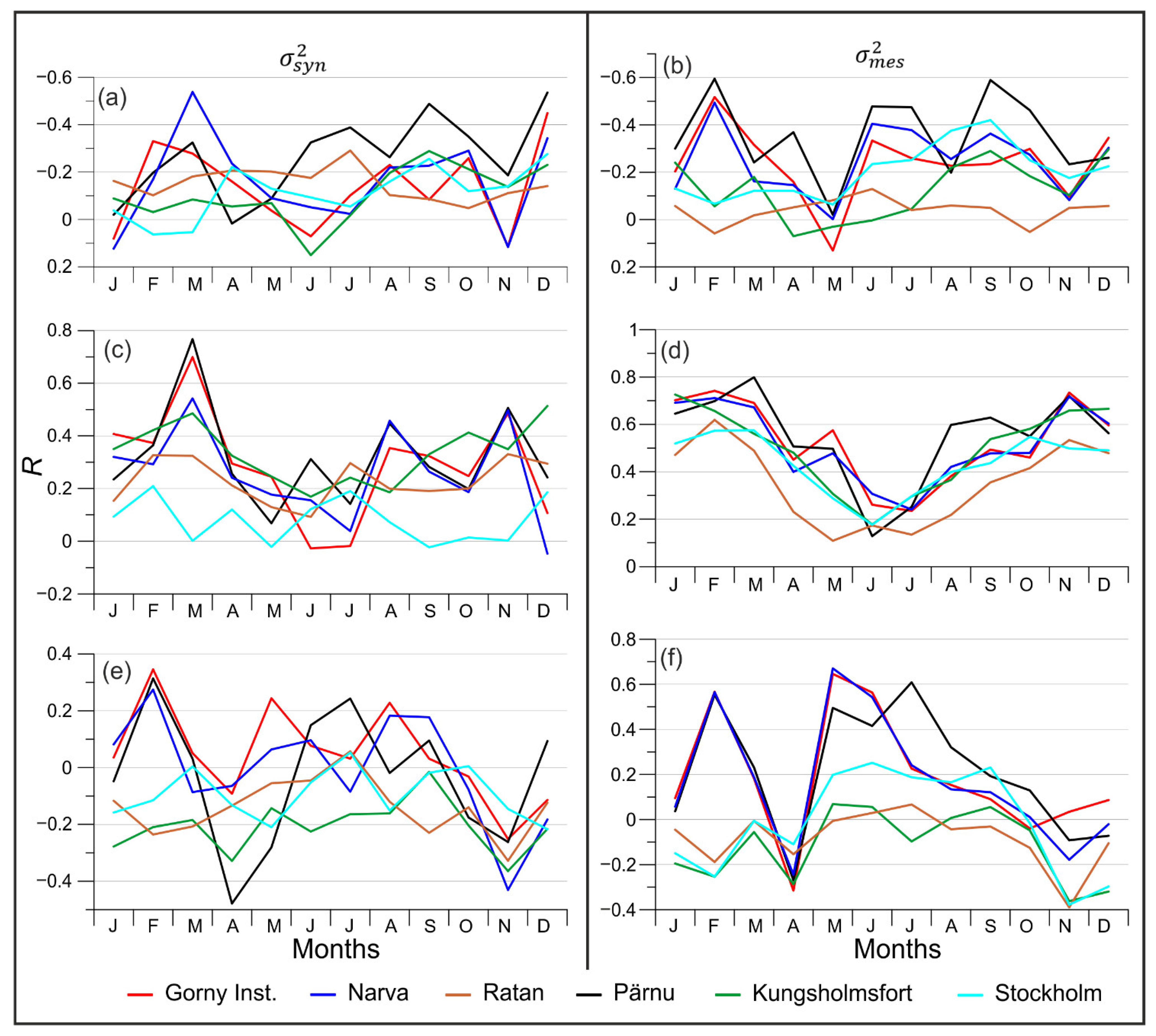
The pairs
−
and
are characterized by negative correlation. The correlation coefficient in the synoptic-scale in all months at all stations varies from 0 to −0.54 without seasonality (
Figure 5a). The correlation coefficient for the mesoscale decreases to −0.60 (
Figure 5b). The eastern coast of the Baltic Sea (Gorny Institute, Narva, Pärnu) is characterized by a correlation coefficient of −0.6 in February, after which the correlation increases to almost zero in May and then decreases in June–July and September. On the western coast of the sea (Swedish stations), on the contrary, a correlation coefficient is about 0 in February and −0.4 in September.
The pairs
and
are characterized by a pronounced seasonal variation with maximum values of the correlation coefficient from November to March and minimum in May–July. For the synoptic scale, a sharp local maximum of the correlation coefficient is achieved in March: up to 0.70 at the Gorny Institute and up to 0.77 at Pärnu (
Figure 5c). The correlation coefficient at Stockholm does not exceed 0.20 for the whole year. For
the seasonal variation of the correlation coefficient has a similar character for all stations (
Figure 5d). The eastern coast of the Baltic is characterized by a high correlation coefficient in January–March (up to 0.74 at the Gorny Institute and up to 0.80 at Pärnu) and a local maximum in November (up to 0.72) and May (up to 0.50–0.58). The seasonal correlation curve for Swedish stations is smoother. The minimum values were found at Ratan. This tide gauge is located in the Gulf of Bothnia, which has a meridional elongation, which, apparently, significantly reduces the effect of the zonal wind on the sea level oscillations in this gulf.
For the pairs
, the correlation coefficient varies from −0.4 to 0.4 during the year, which indicates a lesser influence of the meridional wind on synoptic sea level variations (
Figure 5e). For the Gulf of Finland and the Gulf of Riga, a correlation coefficient is from 0 to 0.4 from January to September, which indicates a small influence of the southerly wind on the formation of sea level variations on the synoptic scale. The correlation coefficient sharply changes its sign to negative in October–December and reaches −0.4 in November, which indicates the influence of the northerly wind on the sea level variations at the synoptic-scale in the autumn.
For the pairs
, the correlation coefficient is higher than for
(
Figure 5f). In February, it is 0.55 for the eastern Baltic coast. The correlation coefficient sharply changes its sign to negative in April (up to −0.3), which again shows an increase in the role of northerly winds in the formation of sea level variations at the mesoscale. The absolute maximum of the correlation coefficient is reached in May, up to 0.65–0.67 in the Gulf of Finland, after which the coefficient decreases, and in November it already has negative values of up to −0.4 on the western Swedish seacoast.
Long-term changes in wind stress over the Baltic Sea are closely related to large-scale atmospheric circulation over the North Atlantic and numerically partially displayed in the North Atlantic Oscillation (NAO) index [
17]. The NAO index is the pressure difference between the Azores maximum and the Icelandic minimum. The essence of the NAO lies in the redistribution of atmospheric masses between the Arctic and the subtropical Atlantic, while the transition from one phase of the NAO to another causes large changes in the wind field, heat, and humidity transfers, in the intensity, number, and trajectories of storms, etc. A positive NAO is characterized by the strong Azores High and Icelandic Low. It is associated with warm and humid winters and strong westerly winds in the Baltic Sea area, which cause sea level rise. A negative NAO (weak Azores High and Icelandic Low) is associated with cold and dry winters, which cause a sea-level decrease. The correlation between the Baltic Sea level and NAO is especially strong in winter [
5,
10].
In the current study, we examined the dependences of interannual changes in the and with changes in the NAO, the Arctic Oscillation (AO), and Scandinavian (SCAND) indices.
The AO is a large-scale mode of climate variability. It is also known as the Northern Hemisphere annular mode [
23]. The AO pattern is characterized by winds circulating counterclockwise around the Arctic at around 55° N latitude. In the positive phase of this pattern, a belt of strong winds circulating the North Pole confines colder air across Polar Regions. When the AO is in a negative phase, this wind belt becomes weaker and more distorted. It allows colder, arctic air masses to penetrate southward more easily, and also the storminess increases into the mid-latitudes.
The Scandinavia pattern SCAND consists of a primary circulation center over Scandinavia, with weaker centers of an opposite sign over Western Europe and eastern Russia [
24,
25]. The positive phase of this pattern is associated with below-average temperatures over western Europe and across central Russia, sometimes reflecting major blocking anticyclones over Scandinavia and western Russia. It is also characterized by above-average precipitation across central and southern Europe and below-average precipitation across Scandinavia.
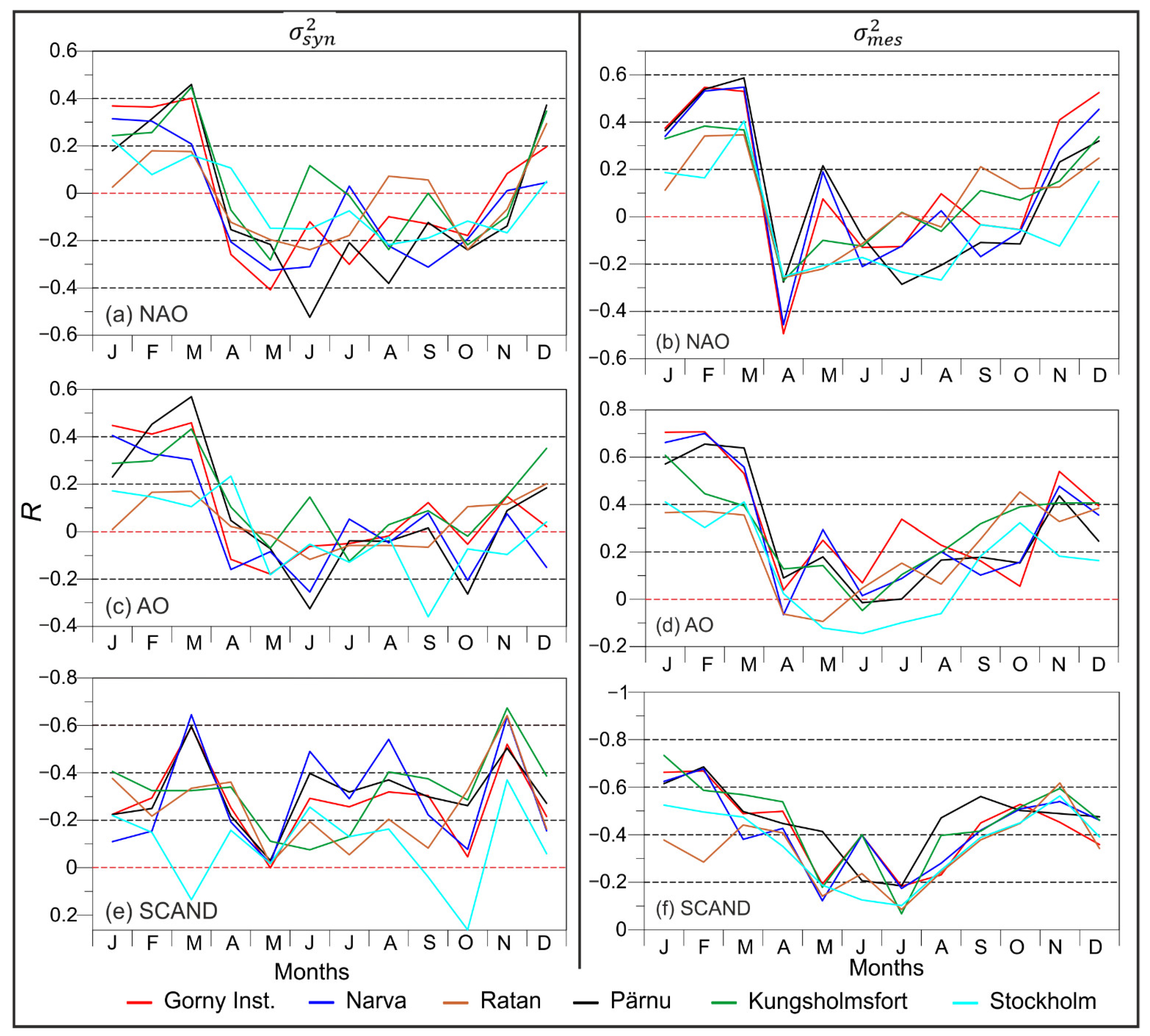
We estimated the correlation coefficients between and and the atmospheric circulation indices in different months. For the pairs of time series − NAO, − NAO, − AO, and − AO, a predominantly positive correlation coefficient is characteristic, while for the pairs − SCAND and − SCAND, the correlation coefficient was mostly negative. This is due to the different directions of the pressure gradient in the calculation of these atmospheric indices. The resultant 95% confidence level for nonzero correlation is 0.21–0.23 for Swedish tide gauges and 0.30–0.31 for short time series (Pärnu, Narva, Gorny Institute).
The largest values of the modulus of the correlation coefficient are observed in the period from November to March (
Figure 6). The correlation approaches zero in the summer. The correlation coefficient at the head of the Gulf of Finland and the Gulf of Riga (Gorny Institute, Narva, and Pärnu) is higher than in the Gulf of Bothnia (Ratan) or in the Baltic Proper (Stockholm). The value of the correlation coefficient for the atmospheric circulation indices and
for individual months is less than for
.
At the Gorny Institute, Narva, and Kungsholmsfort, the correlation coefficient between the variance
and the NAO index reaches the highest values in March, 0.40–0.45 (
Figure 6a). The relationship between
and the AO index at six tide gauges is slightly higher than with NAO. The correlation coefficient between changes in the AO index and
at Pärnu is 0.57 in March (
Figure 6c). The largest values of the modulus of the correlation coefficient are found with the SCAND index (
Figure 6e). At the Gorny Institute, Narva, and Kungsholmsfort, the correlation coefficient with the SCAND index is −0.60–−0.65, and in November, high correlation coefficients between
and the SCAND index are found not only in the Gulf of Finland (up to −0.64) and the Gulf of Riga (−0.50) but also at Ratan (−0.64) and Kungsholmsfort (−0.67). The correlation coefficients between
and the NAO and AO indices in November are rather low at all stations, 0.08–0.15.
The seasonal variations of the correlation coefficient calculated for pairs of time series of
and circulation indices have a similar form: maximum values in winter and about 0.10–0.20 in summer. At the Gorny Institute, Narva, and Pärnu stations, the correlation coefficient between
and the NAO index has the highest values in February–March, 0.55–0.59 (
Figure 6b). The relationship between
and the AO index is even higher in February–March at these stations, up to 0.65–0.70 (
Figure 6d). The SCAND index also shows a high correlation coefficient, but with the opposite sign, −0.69 (
Figure 6f). The correlation coefficient with the SCAND index at Kungsholmsfort in January is −0.73. In November,
a high correlation with all atmospheric indices is observed.
3.4. Interannual Changes in Sea Level Oscillations Variance
The variance of synoptic (
) and mesoscale (
) sea level oscillations changes from year to year. Medvedev [
5] has shown that interannual changes in
are in phase in different areas of the Baltic Sea (Ratan, Stockholm, and Kungsholmsfort) and do not have significant trends from XX to XXI centuries. In the interannual changes in
, no significant trends were found either. Additionally, Medvedev [
5] has shown that if we calculate the trends for observations from 1922 to 2010, then a pronounced positive trend was found at Ratan, Kungsholmsfort, and Stockholm: from 0.04 cm
2/year at Ratan to 0.14 cm
2/year at Kungsholmsfort. In the current study, we investigated the temporal changes of
and
in more detail.
We estimated
and
for each year.
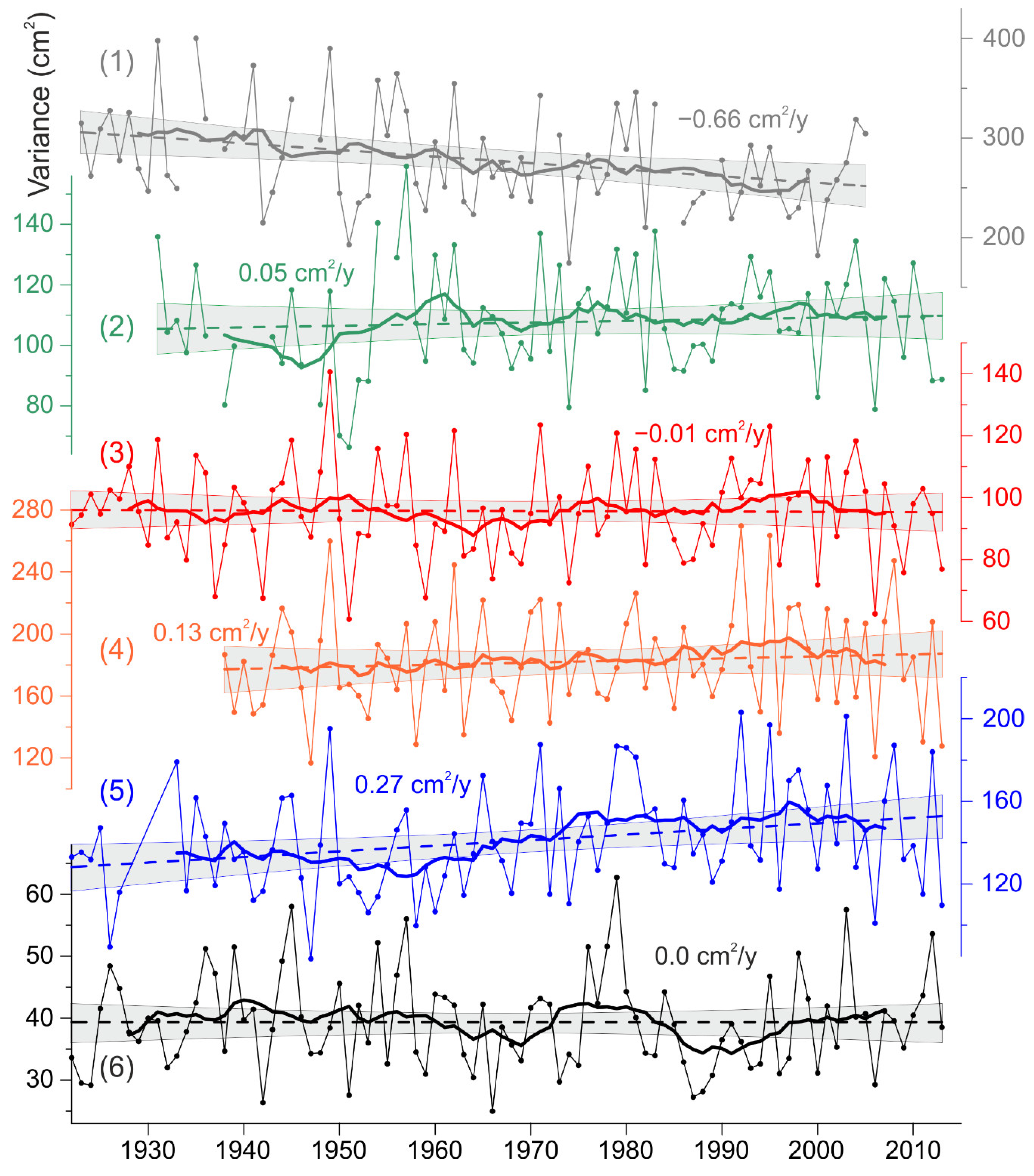
Figure 7 shows interannual changes in
at six tide gauges with long-term observation series from 1922 to 2013. The
values change greatly from year to year. The standard deviation of interannual changes of value of
are from 7 cm
2 at Stockholm to 50 cm
2 at Gedser, which is 16–19% of the long-term average values. A pronounced negative trend of −0.66 cm
2/year was detected at Gedser, i.e.,
decreased by 19% over 90 years. At Ratan, an increase in
with a rate of 0.27 cm
2/year is observed, as a result of which the average value of
over 90 years increased by 17%.
In general, interannual changes in at different tide gauges of the Baltic Sea are similar. The local annual highs and lows of are synchronously observed in different areas of the sea. For example, the local maximum in 1949 and the local minimum in 2006 are expressed both in the southwestern Baltic (Gedser, Klagshamn, Kungsholmsfort) and in the Gulf of Bothnia (Furuogrund and Ratan). For two nearby tide gauges, Ratan and Furuogrund, the correlation coefficient was 0.91. Interannual variations of at Kungsholmsfort are closely related (0.5–0.6) to the southwestern part of the Baltic (Gedser and Klagshamn), in the Gulf of Bothnia (Furuogrund), in the Baltic Proper (Stockholm), and in the Gulf of Riga (Pärnu). Some tide gauges have a relatively weak correlation with the other stations. At Ratan, the correlation coefficient with all the stations under consideration, except Furuogrund, does not exceed 0.40. The Gorny Institute has a correlation of less than 0.20 with most stations, except Gedser (0.40) and Pärnu (0.68). Pärnu has high correlation coefficients with the southwestern Baltic (Gedser, Klagshamn, and Kungsholmsfort) and with the Gorny Institute.
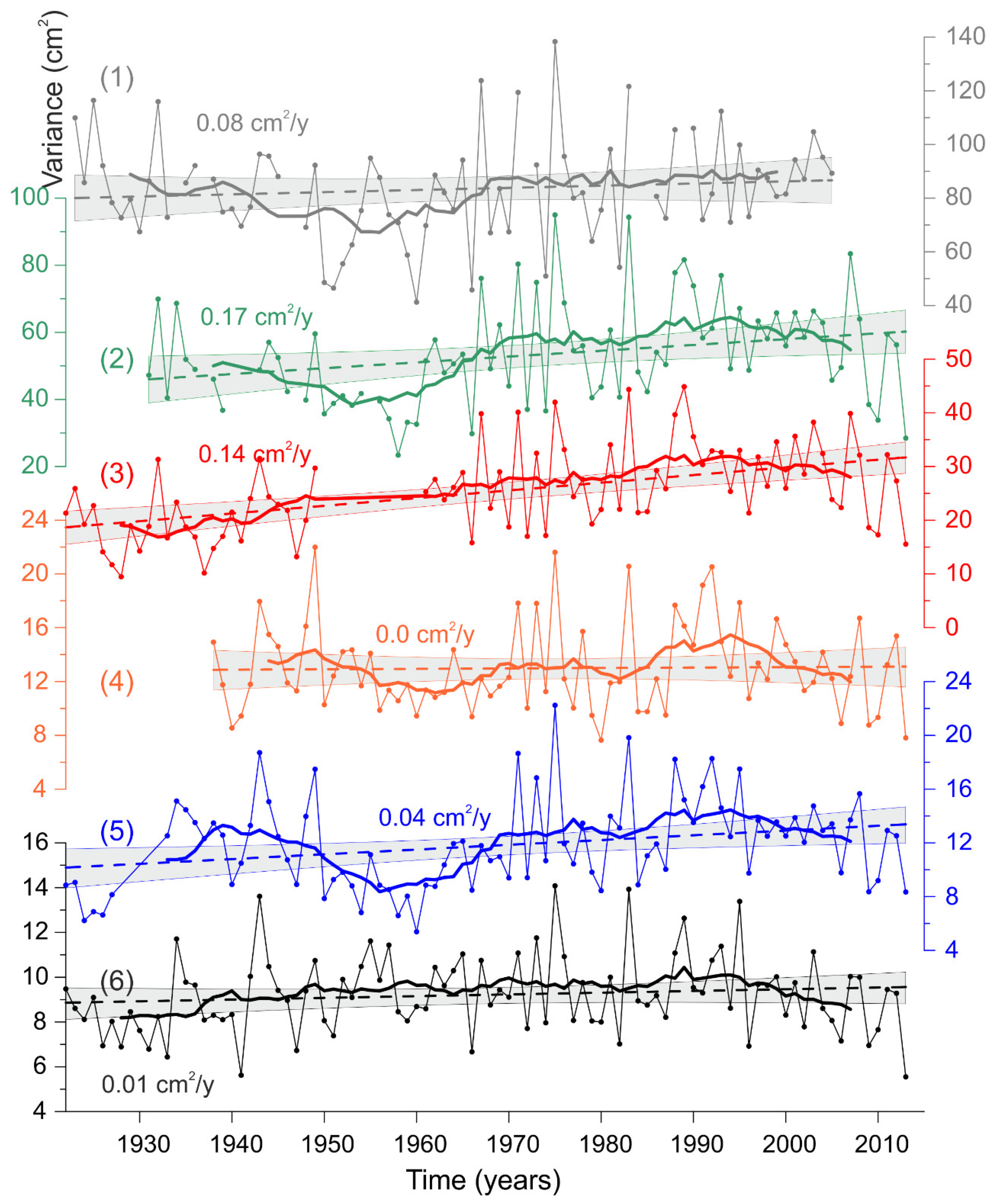
The variance of mesoscale sea level oscillations
changes greatly from year to year (
Figure 8). At Gedser,
changes from 45 to 140 cm
2, and at Ratan from 6 to 22 cm
2. General periods of increase in
, typical for most stations, were observed in 1936–1946, 1970–1979, and 1986–1995. Local minima of
occurred in 1925–1933, 1953–1966, and 1980–1985. After 1996, a negative trend in
is typical for most tide gauges. For the entire observation period (XX–XXI centuries), the absolute estimates of the rate of change of
differ from 0 to 0.17 cm
2/year, and these trends have significant values in relative units (for example, in percent). The trend at Gedser is 0.08 cm
2/year, i.e., over 100 years,
increased by 8 cm
2, which is about 9–10% of the average value of
for this station (85 cm
2). For Klagshamn, 0.17 cm
2/year is about 32% of the average
(53 cm
2), for Ratan up to 36% (average
= 11 cm
2), and for Kungsholmsfort up to 60% (average
= 23 cm
2).
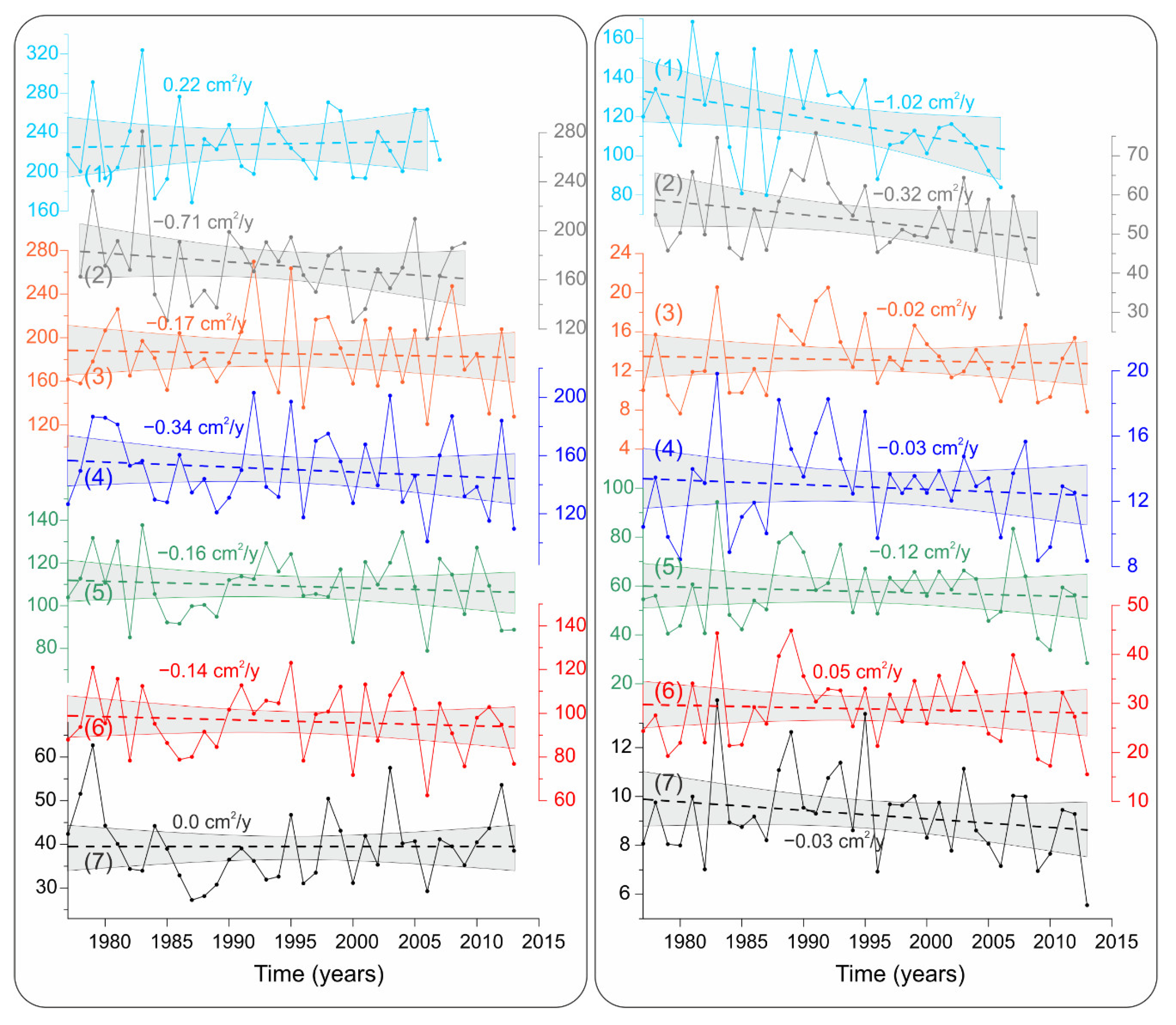
We paid special attention to the change in the values of
and
from 1977–1978 and 2007–2013. Almost all stations have a negative trend in changes in
and
(
Figure 9). The rate of
changes from 0.22 cm
2/year at the Gorny Institute to −0.71 cm
2/year at Pärnu. At most stations,
from 1977 to 2013 decreased by 4–7% from the average for this period. A significant trend was found at Pärnu, where the
decreased from 184 in 1978 to 161 in 2009, i.e., by 23 cm
2, which is 13% of the average value. A local minimum
was observed at all stations from 1985 to 1991.
The rate of
changes from 0.05 cm
2/year at Kungsholmsfort to −1.02 cm
2/year at Gorny Institute. At Ratan, Furuogrund, and Stockholm, the trend was −0.02–0.03 cm
2/year, which ranges from 6% of the average
at Ratan and up to 14% at Stockholm. The most intense decrease in
in 1977–2009 was found at Pärnu, 19% of the average value of
, and for the Gorny Institute, 26%. However, these trends of
and
have low statistical significance (see confidence limits in
Figure 9). This is caused by the short period of time series and the large year-to-year variability of these values.
3.5. Relationship with Atmospheric Circulation, Wind, and Air Pressure Variations
In the current study, using cross-wavelet analysis, we estimated the coherence of changes in
and
with variations in the NAO and SCAND indices on a time-frequency scale. We used monthly data of atmospheric indices and values
,
for two tide gauges: Kungsholmsfort and the Gorny Institute. The coherence wavelet diagrams for
in 1977–2006 have the same structure for NAO–Kungsholmsfort and NAO–Gorny Institute (
Figure 10b,d): high coherence at the annual frequency and periods of 2–4 years. The Kungsholmsfort diagram shows high coherence for periods of 8–16 years in 1977–2006. The coherence between NAO and
is very low for periods longer than 2 years from the 1890s to the 1960s. The NAO and
coherence diagrams for two tide gauges have a similar structure to
for 1977–2006. The long-term series of Kungsholmsfort is characterized by extremely high coherence over periods of more than 20 years for the entire 20th century.
The high coherence area moved from the annual cycle to a period of 1.5–3 years on the diagrams of the SCAND index and the values of
and
. This is found over the entire observation time (
Figure 10e,f,h). Only for the pair SCAND—
at the Gorny Institute is there no increase in coherence for periods longer than 1.5 years.
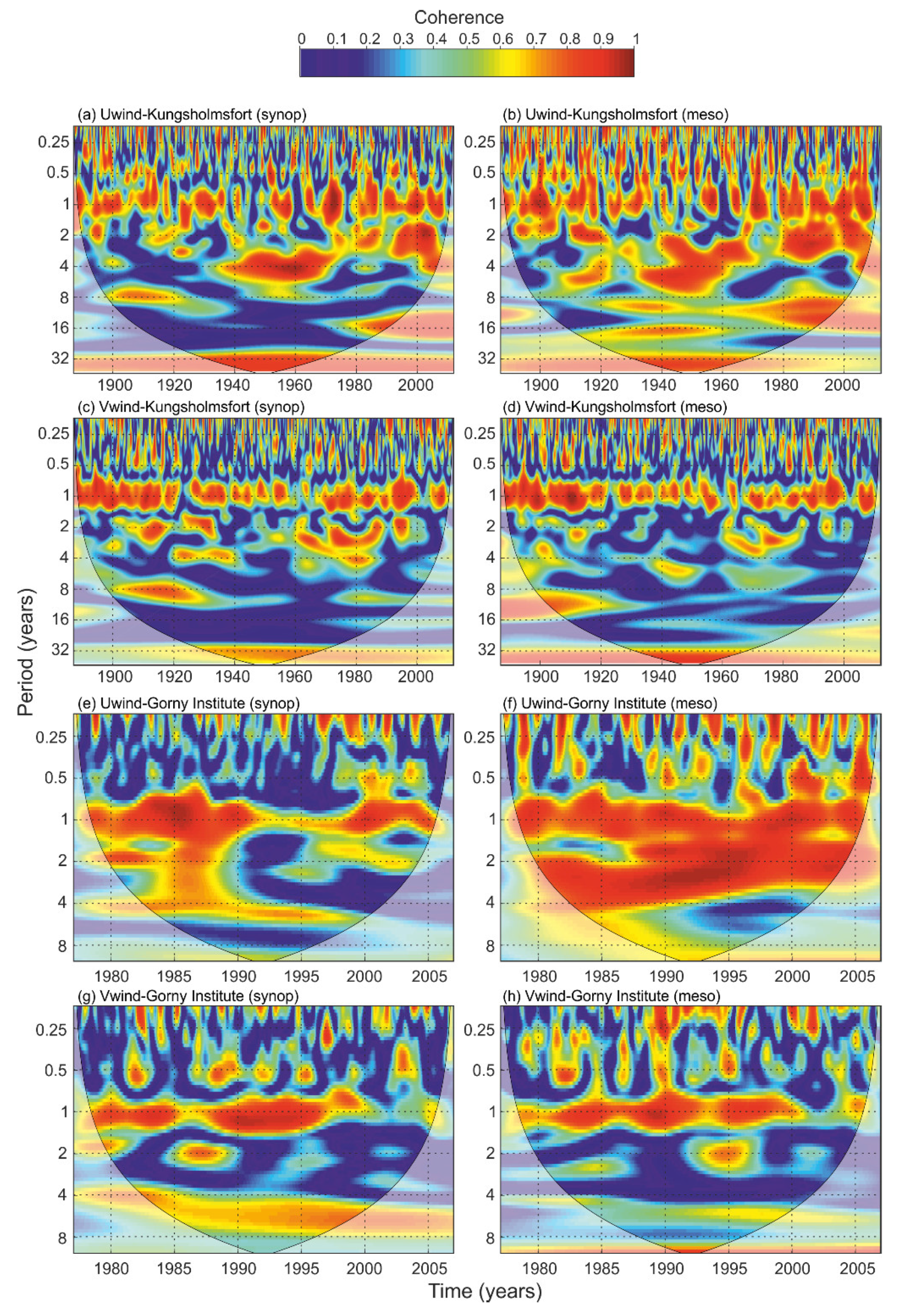
We estimated the wavelet coherence for pairs of monthly mean values of the zonal and meridional wind over the Baltic Sea and the values of
and
at Kungsholmsfort and the Gorny Institute. All diagrams of coherence are characterized by a regular increase of coherence at the annual frequency (
Figure 11). The diagrams of the meridional wind have only local increases of coherence for periods longer than a year (
Figure 11c,d,g,h). The zonal wind diagrams are characterized by wide areas of high coherence for longer than annual periods (
Figure 11a,b,e,f). For the pair of
at the Gorny Institute, an area of high coherence with periods from 0.7 to 4 years is observed throughout the observation period from 1977 to 2006 (
Figure 11f).


