Multivariate Analysis of Water Quality Data for Drinking Water Supply Systems

Abstract

Vulnerability of drinking water supply systems (DWSSs) depends on different factors such as failures, loss of security, man-made threats, and the change and deterioration of supply-water quality. Currently, the lifespan of several DWSSs worldwide has been exceeded, exasperating these issues. The monitoring activity and the transparency of information on water availability and quality are becoming increasingly important in accordance with the national regulations and standards, and with guidelines of the World Health Organization (WHO). These activities can be considered as support and guidance tools for identifying health-related risks, for building a safe management of drinking water supply systems, and for improved user confidence in the consumption of tap water. In this context, in the present work an analysis of the quality monitoring data of DWSSs was carried out using multivariate techniques. The analysis considered several chemical–physical parameters collected in the period 2013–2020 for some DWSSs in the Emilia-Romagna region, Italy. Principal component analysis (PCA) and cluster analysis (CA) methods were used to process and reduce the dimensionality of the data, to highlight the parameters that have the greatest influence on the qualitative state of the supplied water and to identify clusters.

1. Introduction

Water resources are vital to human life and activities. Considering the economic, social, environmental, and public health aspects of water resources, important is the sustainable management of these resources together with the management aspects of drinking water supply systems (DWSSs) [1]. Design and management of DWSSs involve several aspects of research related to optimization models for design, pipe failures, vulnerability, quality, robustness, and resilience [2,3,4,5,6].

Currently, in numerous countries, many DWSSs have exceeded their lifespan and the age of these networks is a factor, contributing to water quality deterioration within the system.

Water quality is monitored through sampling and analysis of a certain number of physical, chemical, and bacteriological parameters at different sampling points; the number and type of monitored parameters, frequency and method of sampling, and monitoring plans are defined according to government regulations.

In EU, the Drinking Water Directive (DWD)—Council Directive 98/83/EC laid down the water quality standards at EU level. On 16 December 2020, the European Parliament formally adopted the revised Drinking Water Directive. The Directive entered in force on January 2021, and Member States will have two years to transpose it into national legislation. Among the innovations present in the revised DWD, there is the assessment of risks associated with distribution, including the domestic distribution, and the effective and transparent communication to users regarding the water quality in order to promote the consumer confidence. An important aspect of the revised DWD is also the need to provide users with simple and accessible information on the availability and quality of tap water, thus improving trust in tap water use and favoring the reduction of bottled water consumption.

For managers and water-supply companies, data analysis and interpretation are important elements for proper DWSSs management. The monitoring data constitute an n-dimensional space characterized by parameters measured and interpreted separately. In this context, the methods of multivariate statistical analysis, such as principal component analysis (PCA), allow for establishing correlations between parameters, and to interpret and analyze the parameters together.

Methods of multivariate statistical analysis have been mainly used for monitoring the quality of surface water [7,8,9,10,11,12,13] and groundwater [14,15,16,17,18,19], although some studies were also carried out on drinking water and DWSSs. Praus (2005) [20] analyzed by multivariate methods a set of data relating the quality monitoring in 126 drinking water samples taken from a city water network in North Moravia, Czech Republic. Through PCA, the dimensionality of the dataset was reduced and the clusters sorted the drinking water samples according to their groundwater and surface water origin. Using principal component analysis and cluster analysis, Jankowska et al. (2017) [21] studied the multivariate correlation among chemical parameters in 11 WDNs of Siedlce County in Poland, and the water networks were grouped based on similar water quality aspects. Quality assessment of three types of drinking water sources in Guinea-Bissau was carried out by [22], considering microbiological and physicochemical parameters. Six water samples were collected from 22 different points considering piped water distribution systems, deep tubewells, and shallow hand-dug wells. Euclidean distance and principal component analysis were used to assess relationship between the microbiological, physical, and chemical parameters considered in the study. Tiouiouine et al. (2020) [23] used PCA to analyze data extracted from the SISE-Eaux database archived since 1990 by the French Regional Health Agency. The authors selected a 10-year period (2006–2016) from the Provence-Alpes-Côte d’Azur region database. PCA was used to synthesize the information and to separate the independent sources of variability.

In this work, a multivariate statistical analysis was carried out considering some DWSSs of the Emilia-Romagna region, Italy. In Italy, the governance of integrated water services has been characterized in recent decades by various regulatory provisions and an evolving political, legal, and institutional framework. Over the years, the fragmentation of the management of this service has not allowed a systematic and organized collection of data on the integrated water service and on the water quality monitoring. Therefore, the lack of such data did not allow for carrying out in Italy many studies on the aspects of water quality and monitoring for DWSSs. Emilia-Romagna, on the other hand, is a region that has implemented over the years a reorganization of the integrated water service by creating a single optimal territorial area governed by an entity, endowed with legal personality under public law and administrative, accounting, and technical autonomy. The management is entrusted to some companies. The reorganization and management of integrated water services in this region has favored the collection and availability of data. In this context, the interest of this work deals with the possibility to perform a multivariate statistical analysis using the sampling data of the regular monitoring carried out by one water-supply company for seven territorial operational districts of the region, at municipal scale. The samplings refer to a large of time period, 2013–2020, and several physical and chemical parameters were considered.

It is worth highlighting that the water supplied is of good quality for all districts and in accordance with standard values. The aim of this paper is use PCA to analyze and reduce the dimensionality of the data acquired during the regular monitoring of the water quality of the DWSSs and to identify correlations between the chemical and physical parameters taken into consideration. Results are used to better interpret these data in support of the DWSSs management activities and investment. Clusters have also been identified using the k-means clustering method. Using this approach, managers can have a global view of water quality in urban areas and identify the parameters that present maximum variance and could be benefit from expanded monitoring.

2. Data and Methods

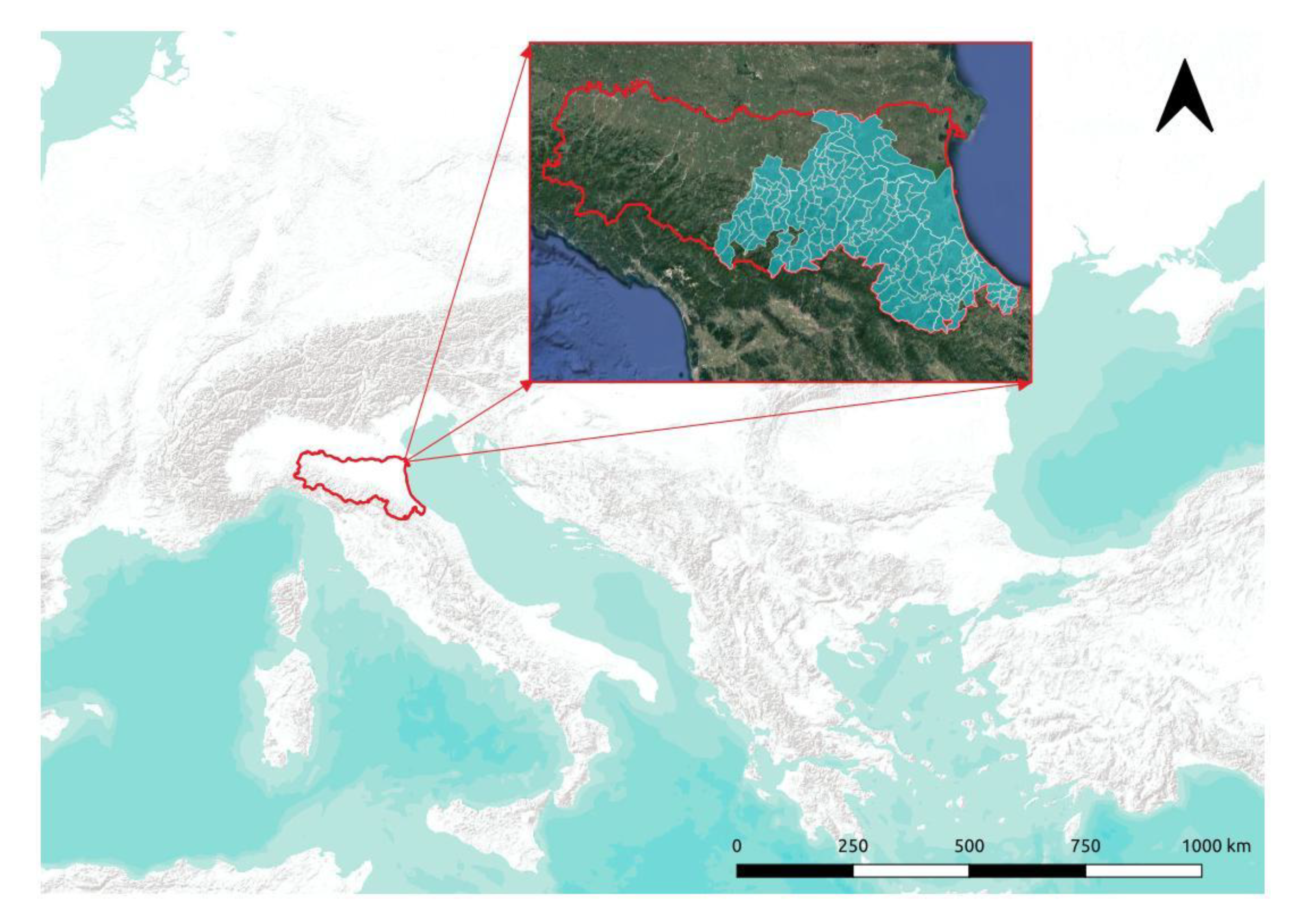
2.1. Case Study Area

The Emilia-Romagna region has a population of about 4.5 million inhabitants and a territorial extension of 22,500 km². The quality data of the DWSSs used for the work presented here concern the regular monitoring carried out by the Hera group, whose basic activity in the water sector concerns management of the Integrated Water Service for many municipalities of the Emilia-Romagna region [24]. The territorial operational districts, the provinces of which the districts are part, the number of municipalities, and some characteristics of the DWSSs managed by Hera S.p.A., whose quality data were used in this study, are indicated in the following table (

Table 1. Territorial operational districts and some characteristics of the DWSSs.

Territorial Operational District	Municipality Managed	Sources of Water	Network Length (km)
Metropolitan city of Bologna	42	groundwater and surface water	9238
District of the Province of Ferrara	11	groundwater and surface water	2514
District of the Province of Forlì-Cesena	30	surface water, groundwater, and springs (smaller share)	4039
District of the Province of Modena	26	groundwater and surface water (smaller share)	4617
District of the Province of Rimini	24	groundwater, followed by surface water and springs (smaller share)	3006
District of the Province of Ravenna	8	surface water	3802
District of the Province of Imola-Faenza	23	surface water	3500

) [25]:

Overall, the quality monitoring data relating to the networks of 164 municipalities were analyzed.

Figure 1 shows the Emilia-Romagna region and all the municipalities of the seven territorial operational districts analyzed.

2.2. Data

Monitoring data were collected from 2013 to 2020 according to Italian and European standards. The regulatory framework consists of:

• Legislative Decree 2 February 2001, no. 31 “Implementation of directive 98/83/EC involving the quality of water for human consumption”;
• Legislative Decree 2 February 2002, no. 27 “Modifications and additions to Legislative Decree 2 February 2001, involving the implementation of directive 98/83/CE on the quality of water for human consumption”;
• Legislative Decree 3 April 2006, no. 152 “Norms on environmental matters”.

The results of 18 physical and chemical parameters were considered and the samples collected from various points of DWSSs from sources to the distribution system, and in drinking-water treatment plants (means of the measurements) [26]. Analyses were carried out according to the actual standardized ISO and EN methods. All the monitoring parameters and standard values are described in

Table 2. Parameters and standard values.

Parameter	Unit	Health-Based Guideline Value WHO	Italian Standard Value
Bicarbonate alkalinity	mg/L	-	-
Total alkalinity	mg/L	-	-
Ammonia	mg/L	-	0.50
Arsenic	µg/L	10	10
Calcium	mg/L	-	-
Free residual chlorine	mg/L	0.2 *	0.2
Chloride	mg/L	-	250
pH	-	-	>6.5–<9.5
Conductivity at 20 °C	μ S/cm a 20 °C	-	2500
Water hardness	°F	-	15–50 **
Fluoride	mg/L	1.5	1.5
Magnesium	mg/L	-	-
Manganese	mg/L	-	50
Nitrate (NO3)	mg/L	50	50
Potassium	mg/L	-	-
Dry residue at 180 °C	mg/L	-	1500 *
Sodium	mg/L	-	200
Sulfate	mg/L	-	250

* Minimum recommended value; ** suggested value range.

.

Among these parameters, for each operational district, a preliminary selection of the variables carrying the most useful information was carried out. The criterion used for the selection of the parameters was based on the relative deviation standard (RDS) together with the evaluation and disposal of variables showing weak correlation with the others.

2.3. Methods

Among multivariate statistical techniques, PCA is probably one of the most popular and used in many different fields. PCA was first introduced by Pearson [27] and its present formalization was developed by Hotelling [28]. PCA allows for the analysis of large datasets that represent observations of several variables that are generally interrelated [29]. Goals of PCA are to extract the most important information from the dataset, reduce dimensionally the dataset, and simplify it, thereby minimizing information loss, allowing for analysis of the structure of observations and variables. This reduction is achieved by transforming original variables to a new set of variables, the so-called principal components, PCs, which are uncorrelated and ordered so that the first few retain most of the variation present in all of the original variables [30]. Computation of the principal components reduces to the solution of an eigenvalue–eigenvector problem for a positive-semidefinite symmetric matrix [29]. PCA can be considered as a rotation of the axes of the original variable coordinate system to new orthogonal axes, called principal axes, such that the new axes coincide with directions of maximum variation of the original observations. PCA can be performed using a method based on the variance–covariance matrix or the correlation matrix. A correlation PCA occurs when variables are measured with different units and a standardization of each variable to the unit norm is carried out.

Considering a data matrix X, PCA provides an approximation of X in terms of the product of two matrices T and P’. These matrices, T and P’, capture the essential data patterns of X. Plotting the columns of T gives a picture of the dominant “object patterns” of X and, analogously, plotting the rows of P’ shows the complementary “variable patterns” [31]:

$$X=T_1{P_1}^{\prime }+T_2{P_2}^{\prime }+\dots T_A{P_A}^{\prime }+E$$

(1)

The columns in T, ta, are the score vectors and the rows in P’, pa, are defined as loading vectors. E is defined as the residual matrix.

For the study described in this paper, the data were normalized to the z score before applying PCA, while the scree plot was used to select the number of PCs [32]. The scree plot shows the number of eigenvalues ordered from largest to smallest, and the number of components defined as the number that appears prior to the elbow of the curve.

Regarding CA, k-means clustering algorithm was used. This algorithm allows for partitioning the data into a certain number of clusters such that a clustering criterion is optimized. The objective of k-means clustering is to minimize the squared error function [33].

To measure the datasets adequacy, the Kaiser–Meyer–Olkin (KMO) test was carried out [34]. A KMO value of 0.5 is considered the smallest value acceptable for PCA.

PCA and CA were performed using the Octave 5.2.0 software, while the KMO test was performed by Python 3.7.9.

3. Results and Discussion

The PCA multivariate method and the k-means clustering were applied to the dataset of each district of the study case. This section describes the results obtained.

For each district, the correlation matrix, the table of eigenvalues of each principal component, the scree plot of PCs, and the georeferenced map of the district with clusters highlighted are included as Supplementary Materials (Annex I–VII).

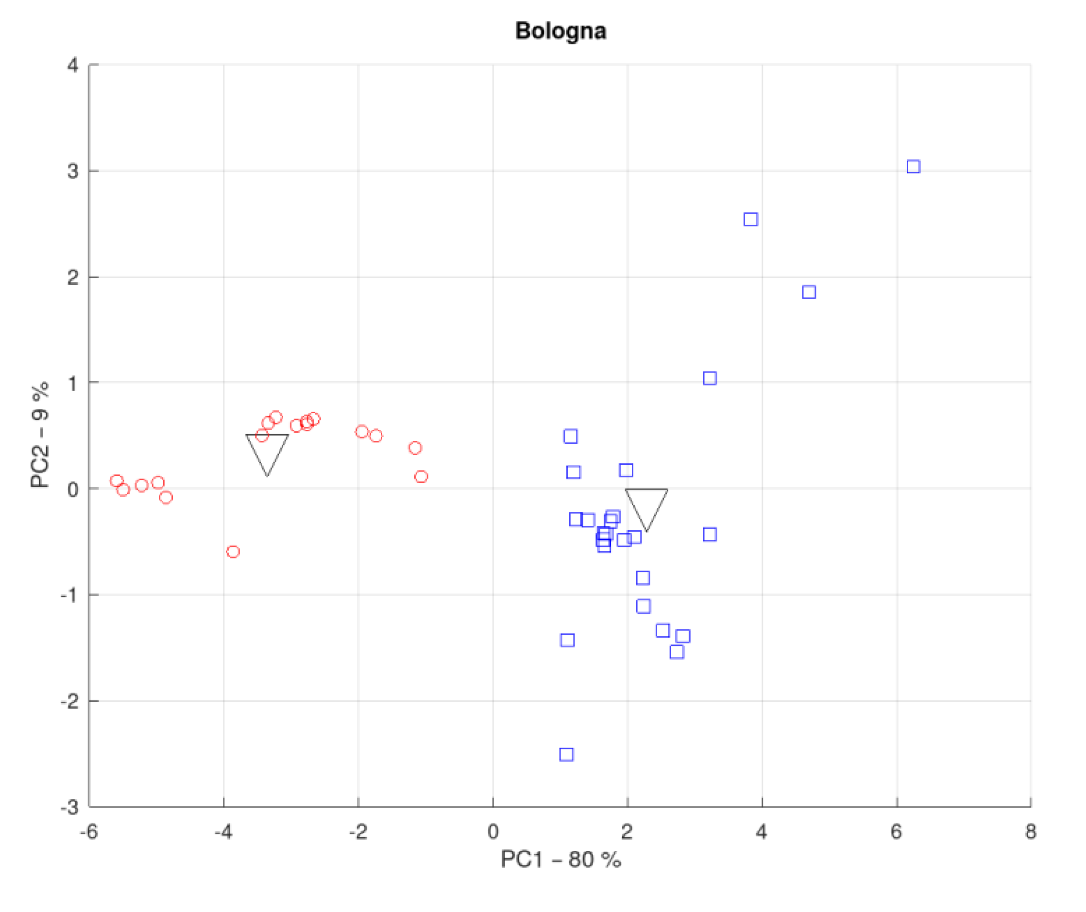
3.1. District of the Metropolitan City of Bologna

As previously mentioned, for this study there were 42 reference municipalities in the area of the metropolitan city of Bologna.

Considering the dataset of this district, 12 parameters were considered: bicarbonate alkalinity, total alkalinity, calcium, chloride, pH, conductivity at 20 °C, water hardness, magnesium, nitrate (NO₃), potassium, dry residue at 180 °C, and sulfate.

A value of 0.69 was obtained by performing the KMO test.

Regarding PCA analysis, two PCs were identified, which explained about 89% of the total variability. The first component PC1 is associated with calcium, chloride, pH, conductivity, water hardness, magnesium, and dry residue. PC2 is mainly composed of bicarbonate alkalinity, total alkalinity, nitrate, and potassium.

Concerning the clustering, two clusters were identified based on PCA scores. The first cluster includes 17 municipalities while the second comprises 25 municipalities. The difference between the clusters is related to the supply systems; the municipalities of the first cluster are served by the same DWSS with supply from surface water, groundwater, and springs, while the municipality of the second cluster are almost all served by the same DWWS as the first cluster, but also by other supply systems (springs, groundwater, and surface water from a lake).

Figure 2 shows the 2D-Score plot considering PC1 vs. PC2 with the two clusters highlighted.

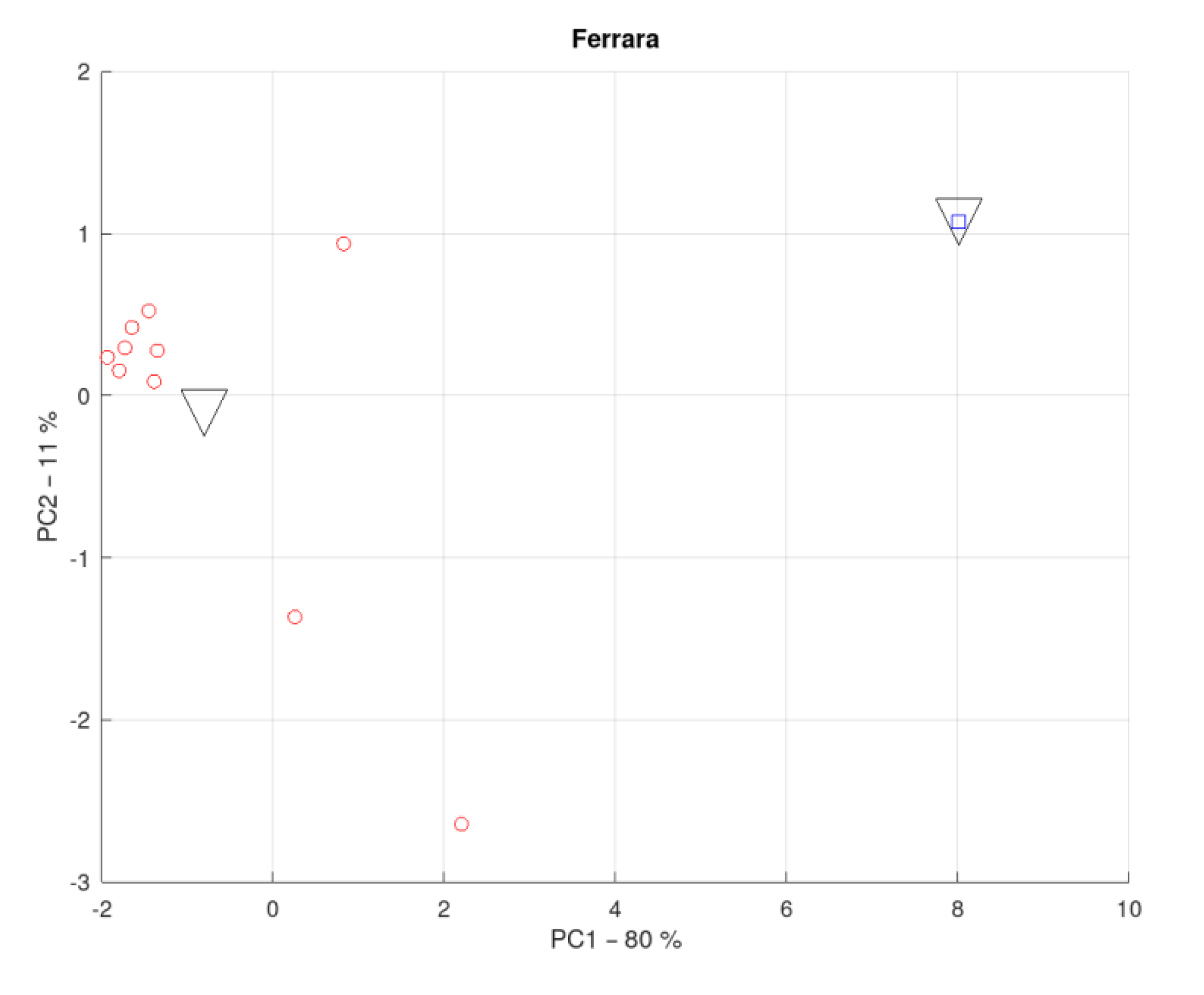
3.2. District of the Province of Ferrara

Regarding the eleven municipalities of this district managed by Hera group, 11 parameters were considered: bicarbonate alkalinity, total alkalinity, calcium, pH, conductivity at 20 °C, water hardness, magnesium, nitrate (NO₃), potassium, dry residue at 180 °C, and sulfate. A value of 0.61 was obtained by performing the KMO test.

For this district, two PCs were identified which explained 91% of the total variability. PC1 explained 80% of the total variability and is mainly associated with bicarbonate alkalinity, total alkalinity, calcium, conductivity, water hardness, magnesium, potassium, dry residue, and sulfate. PC2 (11%) is associated with pH and nitrate.

Regarding the clustering analysis, two clusters were identified; the first groups almost all the municipalities while the second cluster consists of only one municipality (Figure 3).

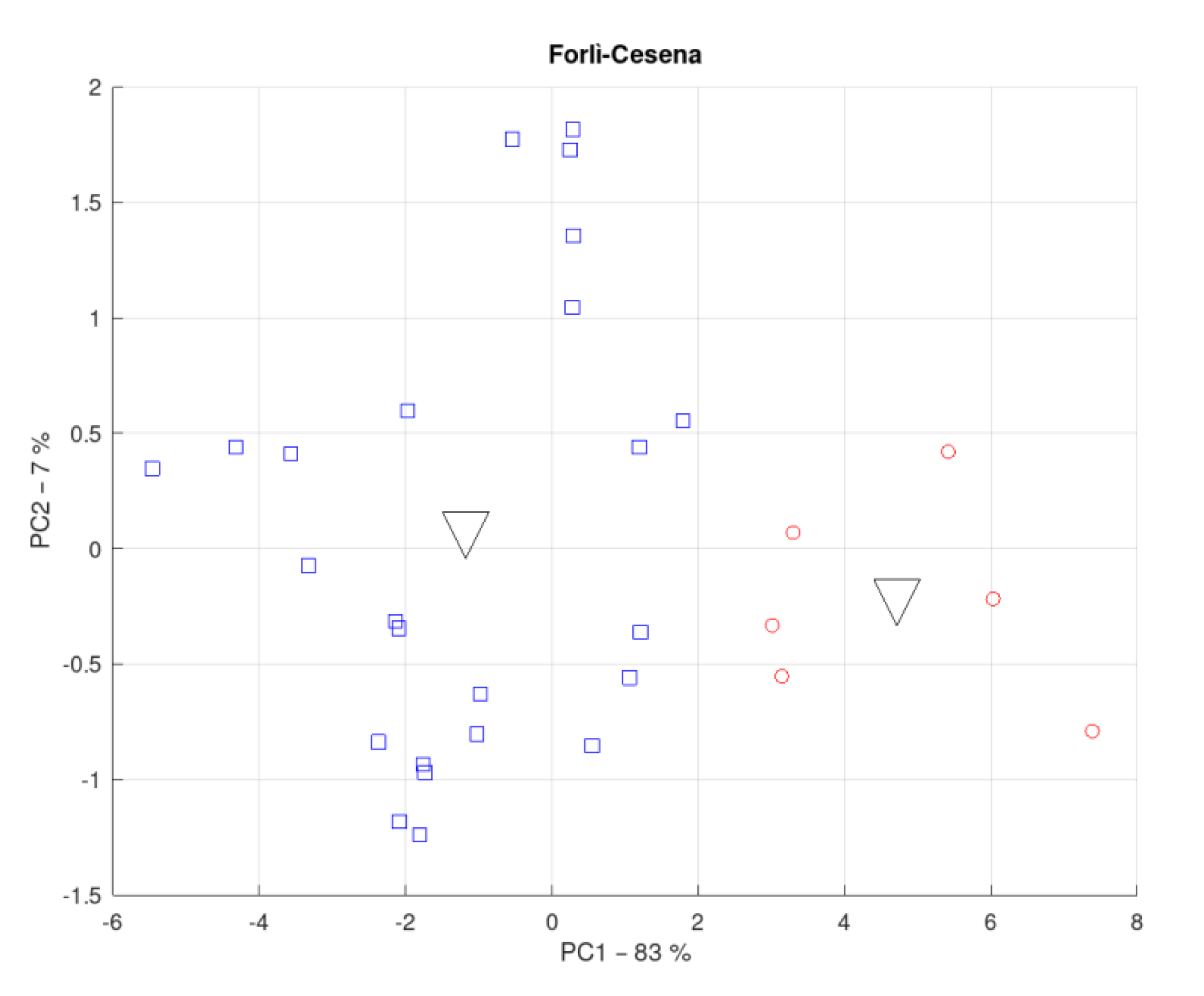
3.3. District of Forlì-Cesena

Regarding the thirty municipalities of the district of Forlì-Cesena, 11 parameters were considered. For this district, the KMO test value is 0.62 and the parameters used were bicarbonate alkalinity, total alkalinity, calcium, pH, conductivity at 20 °C, water hardness, fluoride, magnesium, potassium, dry residue at 180 °C, and sulfate.

With the 90% of the total variability explained, for this district two PCs were identified. PC1 (about 83% of total variability) is composed of bicarbonate alkalinity, total alkalinity, calcium, conductivity, water hardness, magnesium, potassium, dry residue, and sulfate, while PC2 (about 7%) is associated with pH and fluoride.

Regarding the clustering, two clusters were identified; the first cluster groups six municipalities while the second consists of 24. For the largest cluster, most of the water availability (about 63%) derives from the same water source, Lake Ridracoli. For the remaining part, the water supply is also provided by municipal and intermunicipal DWSSs. Regarding the first cluster, the water supply is mainly provided by municipal and intermunicipal DWSSs. These considerations justify the difference between the two clusters and the results obtained.

Figure 4 shows the 2D-Score plot considering PC1 vs. PC2; the same figure also shows the clusters.

3.4. District of the Province of Modena

Regarding this district, 11 parameters were considered.

The result of the KMO test obtained is not very suitable as it is just above the acceptability limit and equal to 0.51, although the variance explained is about 91%. Therefore, the result obtained for the multivariate analysis, in terms of clusters and grouping by similar features, resulted in compatibility with DWWSs schemes and the origin of water sources.

Parameters considered are bicarbonate alkalinity, total alkalinity, calcium, pH, conductivity, magnesium, nitrate, potassium, dry residue, sodium, and sulfate. PC1 (about 77%) is composed of calcium, pH, conductivity, magnesium, nitrate, potassium, and dry residue, while PC2 explained about 15% of the total variability and is associated with bicarbonate alkalinity, total alkalinity, sodium, and sulfate.

Regarding the clustering, three clusters were identified; the first cluster groups nine municipalities while the second consists of 12 municipalities, and the last cluster is composed of five municipalities. For the first and second cluster, all municipalities are served by the same two DWSSs; similarly, in the case of the third cluster, almost all the municipalities are served by the same DWSS. It is worth noting that two municipalities of the first cluster are also interconnected with DWSSs of the third cluster.

The 2D-Score plot considering PC1 vs. PC2 with highlighted clusters is shown in Figure 5.

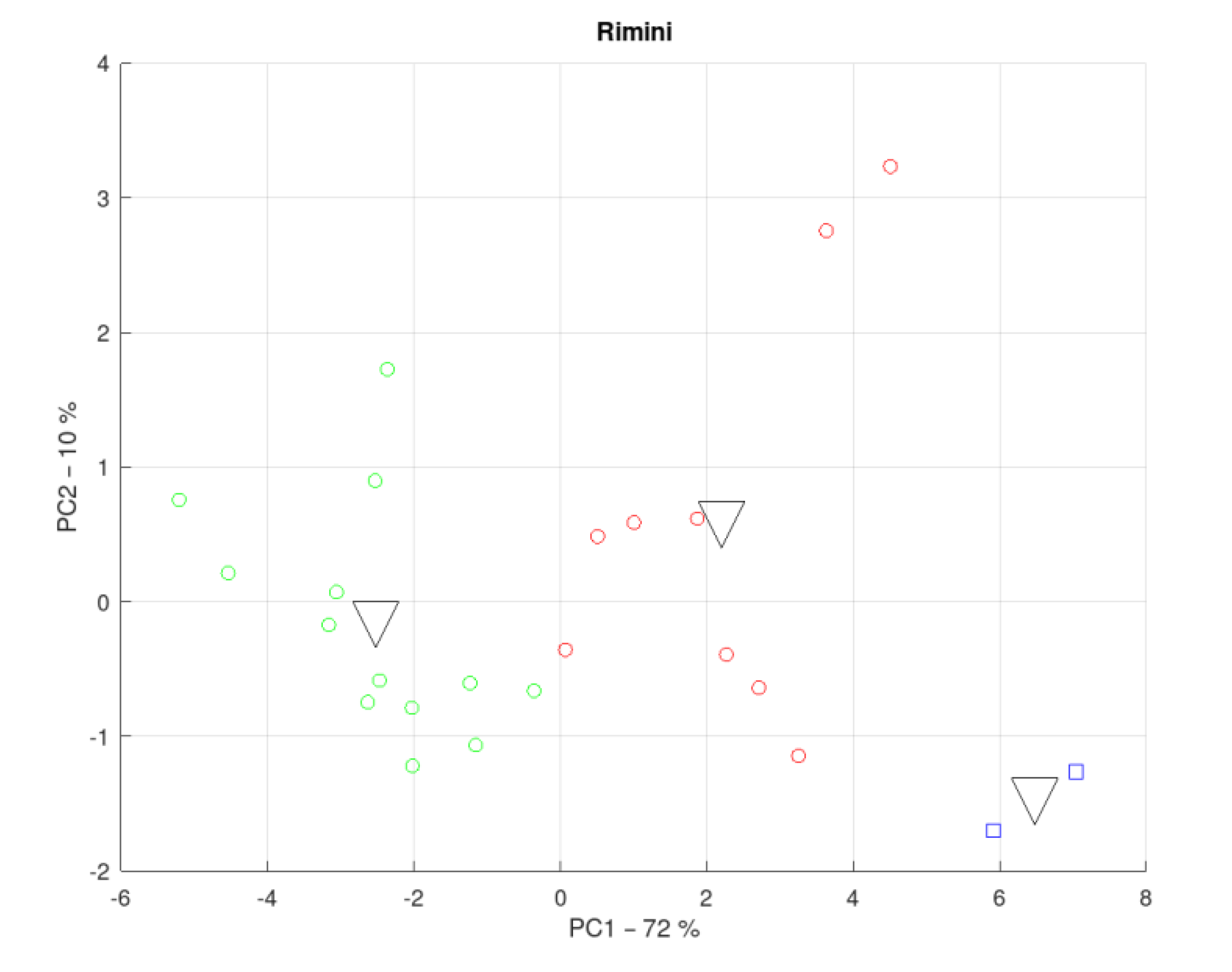
3.5. District of the Province of Rimini

Regarding this district, 15 parameters were considered. The result of the KMO test is 0.6.

Parameters considered are bicarbonate alkalinity, total alkalinity, calcium, free residual chlorine, chloride, pH, conductivity, water hardness, fluoride, magnesium, potassium, dry residue, sodium, and sulfate. PC1 explained about 72% of the total variability and it is associated with conductivity, water hardness, magnesium, potassium, dry residue, sodium, and sulfate; PC2 explained about 10% of the total variability and it is composed of bicarbonate alkalinity, total alkalinity, calcium, free residual chlorine, chloride, pH, fluoride, and nitrate.

Three clusters were identified; the first cluster groups nine municipalities, the second consists of two municipalities, and the last cluster groups 13 municipalities. In general, the entire area is served by two large DWSSs with supply from two lakes (one of which is used only in summer). In addition to these supplies, the water supply for the various municipalities is also integrated with wells. The differences between the three clusters are due to the different wells that provide water resources to the municipalities of each cluster.

Figure 6 shows the 2D-Score plot considering PC1 vs. PC2 and clusters.

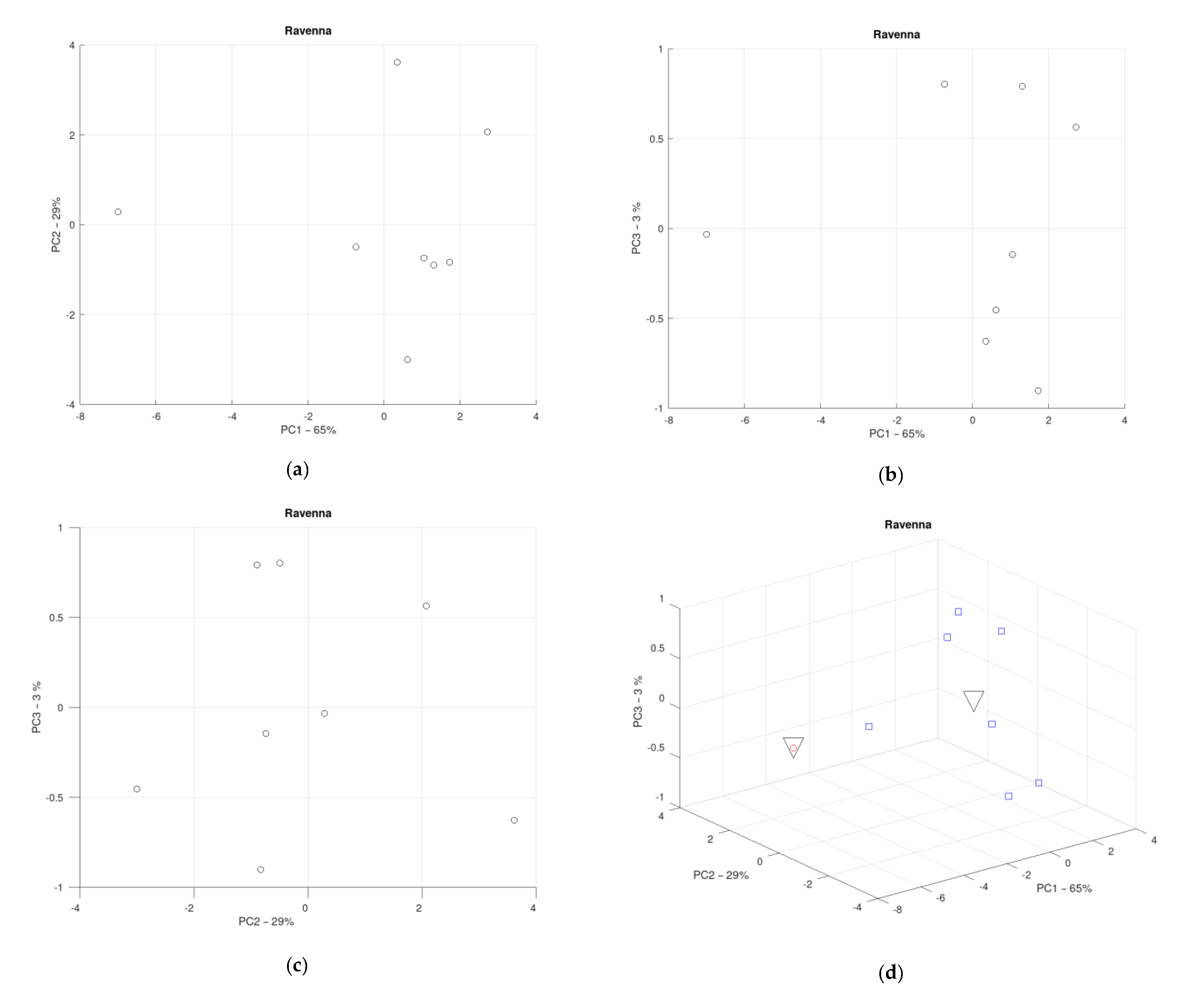
3.6. District of the Province of Ravenna

For this area, 14 parameters were considered: bicarbonate alkalinity, total alkalinity, calcium, chloride, pH, conductivity, water hardness, magnesium, manganese, nitrate, potassium, dry residue, sodium, and sulfate.

The KMO test value is 0.62 while regarding PCA analysis, three PCs were identified, which explain about 97% of the total variability. PC1 is associated with conductivity, water hardness, magnesium, potassium, dry residue and sulfate, while PC2 is composed by bicarbonate alkalinity, total alkalinity, calcium, manganese, and nitrate. Finally, PC3 is associated with chloride, pH, and sodium.

Regarding the clustering, two clusters were identified; in the largest cluster, the six municipalities are mainly served by the same DWSS while the two municipalities of the other cluster differ. In addition to being served by the same DWSS, it is served by about 60% through another water supply scheme.

The 2D-Score plot considering PC1 vs. PC2, PC1 vs. PC3, and PC2 vs. PC3, and the 3D-score plot of the three principal components and clusters are shown in Figure 7.

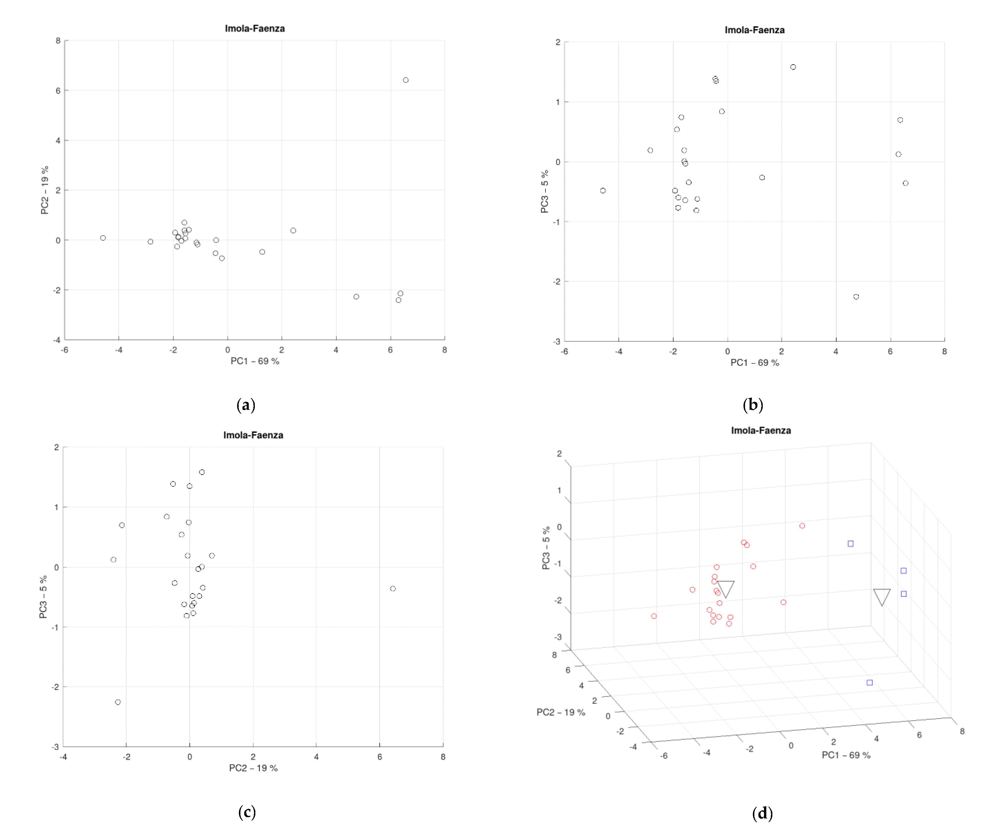
3.7. District of Imola-Faenza

Regarding this district, PCA was carried out considering a total of 14 parameters: bicarbonate alkalinity, total alkalinity, calcium, chloride, pH, conductivity, water hardness, fluoride, magnesium, nitrate, potassium, dry residue, sodium, and sulfate. For this district, as for that of Modena, the KMO test value of 0.56 is not suitable, although, also in this case, the total explained variability is equal to 94%.

Using PCA, the 14 parameters were reduced to three PCs. PC1 is mainly associated with bicarbonate alkalinity, total alkalinity, calcium, conductivity, water hardness, magnesium, and dry residue. PC2 is associated with chloride, fluoride, potassium, and sulfate while PC3 is related to pH and nitrate.

Using the k-means clustering method, two clusters were identified of which the first cluster groups 19 municipalities while the second consists of only four municipalities.

Regarding this cluster, it is worth highlight that three municipalities of the first cluster use waters from the same drinking water treatment plant and one also uses water resources from the DWSS of the largest municipality, the city of Imola. Within the second cluster, the values obtained for one municipality also differ more in relation to the use of water from wells located in the same municipality territory.

Figure 8 shows the 2D-Score plot considering PC1 vs. PC2, PC1 vs. PC3, and PC2 vs. PC3, and the 3D-score plot of the three principal components and clusters.

It is worth noting that overall, for all of the districts, the discarded parameters were ammonium, arsenic, free residual chlorine, and manganese, followed for almost all the districts by fluoride, chloride, and sodium.

Regarding PCA results, for most districts two PCs were identified, except for two districts in which three PCs were identified. PCs explained high percentages of total variability, between 82% and 97%.

The cluster analysis allowed for grouping the municipalities according to similar features in accordance with DWSSs and source origins of the water in an area where the water supply schemes are complex and interconnected.

The districts of Rimini and Ravenna show similar results in terms of discarded and most influential parameters; in particular, conductivity, water hardness, magnesium, potassium, dry residue, and sulfate results are the most influential parameters for these districts. Similar consideration concerns the districts of Bologna, Ferrara, and Forlì-Cesena. These results are related to the origin of water resources and to the interconnected schemes.

4. Conclusions

In this study, the water quality of several DWSSs that provide water for 164 municipalities was analyzed using multivariate methods. In particular, PCA and CA were used to carry out a comprehensive evaluation of the water quality monitoring data, to extract the parameters that most affect water quality and its variation, and to identify clusters in relation to similar characteristics. In this paper, the analysis was performed considering seven districts characterized by complex and interconnected DWSSs. In general, considering all the districts, albeit with the necessary differences, the parameters that most influence the variation in the water resource quality are mainly conductivity, water hardness, magnesium, and dry residue, followed by bicarbonate alkalinity, total alkalinity, calcium, and sulfate.

It is worth highlighting that similar results in terms of the most influential parameters are found for the districts of Bologna, Ferrara, and Forlì-Cesena, which are justified by the interconnection of the DWSSs and the similar types of water sources. Similar results and considerations occur for the districts of Rimini and Ravenna.

Considering each district, the dimensionality of the dataset was reduced to two or three PCs, and the use of CA also allowed for the identification of various clusters. These groups are confirmed and justified in relation to the DWSSs that serve the municipalities, and to the origin of the water supply sources.

The study presented here and the results described aimed at illustrating the usefulness of the PCA method for analyzing and better interpreting complex datasets by reducing their dimensionality and obtaining information on the parameters that have the greatest influence on the variation of water quality. In the same way, the use of CA can be useful to create maps and to group monitoring sites, water supply schemes, water supply sources, and, as in the case of this study, cluster municipalities served by the same DWSSs with similar characteristics. The use and the combination of these methods can be a useful tool for managers and companies to better interpret monitoring data, for the management and monitoring activities, and can lead to improved knowledge concerning the DWSSs, especially where there are complex interconnected schemes and, in case of inadequate knowledge, of the entire water system infrastructure. Finally, considering the growing use of SCADA systems and the transition of DWSSs to cyber–physical systems, the interest of multivariate statistical methods also concerns the prospect of being able to use this approach for the analysis and interpretation of the large amount of data made available by this new type of smart technology system.

References

1. Maiolo, M.; Pantusa, D. Sustainable Water Management Index, SWaM_Index. Cogent Eng. 2019, 6, 1603817. [Google Scholar] [CrossRef]
2. Zhuang, B.; Lansey, K.; Kang, D. Resilience/Availability Analysis of Municipal Water Distribution System Incorporating Adaptive Pump Operation. J. Hydraul. Eng. 2013, 139, 527–537. [Google Scholar] [CrossRef]
3. Herrera, M.; Abraham, E.; Stoianov, I. A Graph-Theoretic Framework for Assessing the Resilience of Sectorised Water Distribution Networks. Water Resour. Manag. 2016, 30, 1685–1699. [Google Scholar] [CrossRef] [Green Version]
4. Diao, K.; Sweetapple, C.; Farmani, R.; Fu, G.; Ward, S.; Butler, D. Global resilience analysis of water distribution systems. Water Res. 2016, 106, 383–393. [Google Scholar] [CrossRef] [Green Version]
5. Maiolo, M.; Mendicino, G.; Pantusa, D.; Senatore, A. Optimization of Drinking Water Distribution Systems in Relation to the Effects of Climate Change. Water 2017, 9, 803. [Google Scholar] [CrossRef]
6. Monsefa, H.; Naghashzadegana, M.; Jamalia, A.; Farmani, R. Comparison of evolutionary multi objective optimization algorithms in optimum design of water distribution network. Ain Shams Eng. J. 2019, 10, 103–111. [Google Scholar] [CrossRef]
7. Sophocleous, S.; Savi, D.; Kapelan, Z. Leak Localization in a Real Water Distribution Network Based on Search-Space Reduction. J. Water Resour. Plan. Manag. 2019, 145, 04019024. [Google Scholar] [CrossRef]
8. Singh, K.P.; Malik, A.; Sinha, S. Water quality assessment and apportionment of pollution sources of Gomti river (India) using multivariate statistical techniques—A case study. Anal. Chim. Acta 2005, 538, 355–374. [Google Scholar] [CrossRef]
9. Gvozdić, V.; Brana, J.; Malatesti, N.; Roland, D. Principal component analysis of surface water quality data of the River Drava in eastern Croatia (24 year survey). J. Hydroinform. 2012, 14, 1051–1060. [Google Scholar] [CrossRef] [Green Version]
10. Garcia, C.A.B.; Garcia, H.L.; Mendonça, M.C.S.; Ferreira da Silva, A.; do Patrocínio Hora Alves, J.; Lopes da Costa, S.S.; Araújo, G.O.; Santos Silva, I. Assessment of water quality using principal component analysis: A case study of the açude da Macela, Sergipe, Brazil. Water Resour. 2017, 3, 690–700. [Google Scholar]
11. Mohanty, C.R.; Nayak, S.K. Assessment of seasonal variations in water quality of Brahmani river using PCA. Adv. Environ. Res. 2017, 6, 53–65. [Google Scholar] [CrossRef]
12. Yang, W.; Zhao, Y.; Wang, D.; Wu, H.; Lin, A.; He, L. Using Principal Components Analysis and IDW Interpolation to Determine Spatial and Temporal Changes of Surface Water Quality of Xin’anjiang River in Huangshan, China. Int. J. Environ. Res. Public Health 2020, 17, 2942. [Google Scholar] [CrossRef]
13. Ioele, G.; De Luca, M.; Grande, F.; Durante, G.; Trozzo, R.; Crupi, C.; Ragno, G. Assessment of Surface Water Quality Using Multivariate Analysis: Case Study of the Crati River, Italy. Water 2020, 12, 2214. [Google Scholar] [CrossRef]
14. Mahapatra, S.S.; Sahu, M.; Patel, R.K.; Panda, B.N. Prediction of Water Quality Using Principal Component Analysis. Water Qual. Expo. Health 2012, 4, 93–104. [Google Scholar] [CrossRef]
15. Zhao, Y.; Xia, X.; Yang, Z.; Wang, F. Assessment of water quality in Baiyangdian Lake using multivariate statistical techniques. Procedia Environ. Sci. 2012, 13, 1213–1226. [Google Scholar] [CrossRef] [Green Version]
16. Usman, U.N.; Toriman, M.E.; Juahir, H.; Abdullahi, M.G.; Rabiu, A.A.; Isiyaka, H. Assessment of Groundwater Quality Using Multivariate Statistical Techniques in Terengganu. Sci. Technol. 2014, 4, 42–49. [Google Scholar] [CrossRef]
17. Marghade, D.; Malpe, D.B.; Rao, N.S. Identification of controlling processes of groundwater quality in a developing urban area using principal component analysis. Environ. Earth Sci. 2015, 74, 5919–5933. [Google Scholar] [CrossRef]
18. McLeod, L.; Bharadwaj, L.; Epp, T.; Waldner, C.L. Use of Principal Components Analysis and Kriging to Predict Groundwater-Sourced Rural Drinking Water Quality in Saskatchewan. Int. J. Environ. Res. Public Health 2017, 14, 1065. [Google Scholar] [CrossRef] [Green Version]
19. Chai, Y.; Xiao, C.; Li, M.; Liang, X. Hydrogeochemical Characteristics and Groundwater Quality Evaluation Based on Multivariate Statistical Analysis. Water 2020, 12, 2792. [Google Scholar] [CrossRef]
20. Praus, P. Urban water quality evaluation using multivariate analysis. Acta Montan. Slovaca 2007, 12, 150–158. [Google Scholar]
21. Radzka, E.; Jankowska, J.; Rymuza, K. Principal Component Analysis and Cluster Analysis in Multivariate Assessment of Water Quality. J. Ecol. Eng. 2017, 18, 92–96. [Google Scholar] [CrossRef] [Green Version]
22. Bancessi, A.; Catarino, L.; Silva, M.J.; Ferreira, A.; Duarte, E.; Nazareth, T. Quality Assessment of Three Types of Drinking Water Sources in Guinea-Bissau. Int. J. Environ. Res. Public Health 2020, 17, 7254. [Google Scholar] [CrossRef] [PubMed]
23. Tiouiouine, A.; Yameogo, S.; Valles, V.; Barbiero, L.; Dassonville, F.; Moulin, M.; Bouramtane, T.; Bahaj, T.; Morarech, M.; Kacimi, I. Dimension Reduction and Analysis of a 10-Year Physicochemical and Biological Water Database Applied to Water Resources Intended for Human Consumption in the Provence-Alpes-Côte d’Azur Region, France. Water 2020, 12, 525. [Google Scholar] [CrossRef] [Green Version]
24. Hera Group. Available online: https://eng.gruppohera.it (accessed on 16 November 2020).
25. Atersir. Agenzia Territoriale dell’Emilia-Romagna per i Servizi Idrici e Rifiuti (Territorial Agency of Emilia-Romagna for Water and Waste Services). Available online: https://www.atesir.it/argomento/servizio-idrico (accessed on 14 January 2021).
26. Hera Group. Water Quality Reports and Archive. Available online: https://www.gruppohera.it/gruppo/attivita_servizi/business_acqua/qualità/qualita_acqua_hera_qualita_media_comuni/ (accessed on 12 January 2021).
27. Pearson, K. On lines and planes of closest fit to systems of points in space. Philos. Mag. 1901, 6, 559–572. [Google Scholar] [CrossRef] [Green Version]
28. Hotelling, H. Analysis of a complex of statistical variables into principal components. J. Educ. Psychol. 1033, 25, 417–441. [Google Scholar]
29. Abdi, H.; Williams, L.J. Principal Component Analysis. In Wiley Interdisciplinary Reviews: Computational Statistics; Wiley: Hoboken, NJ, USA, 2010; p. 2. [Google Scholar] [CrossRef]
30. Jolliffe, I.T. Princypal Component Analysis, 2nd ed.; Springer: New York, NY, USA, 2002; ISBN 0-387-95442-2. [Google Scholar]
31. Wold, S. Principal Component Analysis. In Chemometrics and Intelligent Laboratory Systems; Elsevier Science Publishers: Amsterdam, The Netherlands, 1987; Volume 2, pp. 37–52, Printed in The Netherlands. [Google Scholar]
32. Cattel, R.D. The scree test for the number of factors. Multivar. Behav. Res. 1966, 1, 245–276. [Google Scholar] [CrossRef] [PubMed]
33. Likas, A.; Vlassis, N.; Verbeek, J. The global k-means clustering algorithm. Pattern Recognit. 2003, 36, 451–461. [Google Scholar] [CrossRef] [Green Version]
34. Kaiser, H.F. A second generation little jiffy. Psychometrika 1970, 35, 401–415. [Google Scholar] [CrossRef]
Figure 1. Case study area: the Emilia-Romagna region and all the municipalities of the seven districts analyzed.
Water 13 01766 g001
Figure 2. District of the metropolitan city of Bologna 2D-Score plot showing PC1 vs. PC2 with clusters highlighted: first cluster in red and the second cluster in blue.
Water 13 01766 g002
Figure 3. District of Ferrara 2D-Score plot showing PC1 vs. PC2 with clusters highlighted: first cluster in red and the second cluster in blue.
Water 13 01766 g003
Figure 4. District of Forlì-Cesena 2D-Score plot showing PC1 vs. PC2 with clusters highlighted: first cluster in red and the second cluster in blue.
Water 13 01766 g004
Figure 5. District of Modena 2D-Score plot showing PC1 vs. PC2 with clusters highlighted: first cluster in red and second cluster in blue.
Water 13 01766 g005
Figure 6. District of Rimini 2D-Score plot showing PC1 vs. PC2 and clusters: first cluster in red, second cluster in blue, and third cluster in green.
Water 13 01766 g006
Figure 7. District of Ravenna 2D-Score plot showing PC1 vs. PC2 (a), PC1 vs. PC3 (b), PC2 vs. PC3 (c), and the 3D-score plot of the three principal components and clusters: first cluster in red, second cluster in blue, and the third cluster in green (d).
Water 13 01766 g007
Figure 8. District of Imola-Faenza 2D-Score plot showing PC1 vs. PC2 (a), PC1 vs. PC3 (b), PC2 vs. PC3 (c), and 3D-score plot of the three principal components and clusters: first cluster in red and the second cluster in blue (d).
Water 13 01766 g008