Imaging the Structure and the Saltwater Intrusion Extent of the Luy River Coastal Aquifer (Binh Thuan, Vietnam) Using Electrical Resistivity Tomography

Abstract

With the growing population and the adverse effects of climate change, the pressure on coastal aquifers is increasing, leading to a larger risk of saltwater intrusion (SI). SI is often complex and difficult to characterize from well data only. In this context, electrical resistivity tomography (ERT) can provide high-resolution qualitative information on the lateral and vertical distribution of salinity. However, the quantitative interpretation of ERT remains difficult because of the uncertainty of petrophysical relationships, the limitations of inversion, and the heterogeneity of aquifers. In this contribution, we propose a methodology for the semiquantitative interpretation of ERT when colocated well data are not available. We first use existing wells to identify freshwater zones and characterize the resistivity response of clayey deposits. Then, we approximate the formation factor from water samples collected in the vicinity of ERT data to derive a resistivity threshold to interpret the saline boundary. We applied the methodology in the shallow aquifers of the Luy River in the Binh Thuan province, Vietnam, where water resources are under pressure due to agricultural, aquacultural, and industrial production. Twenty-one ERT profiles were collected and revealed a much larger intrusion zone, compared to the previous study. Saltwater is present in lowland areas of the left bank over almost the whole thickness of the aquifer, while the right bank is constituted of sand dunes that are filled with freshwater. At a larger distance from the sea, a complex distribution between fresh and saltwater is observed. Our methodology could be applied to other heterogeneous aquifers in the absence of a dense monitoring network.

1. Introduction

Saltwater intrusion (SI) occurs along shores and results from the interaction between seawater and coastal aquifers through different processes, such as tidal mixing, water density effects, surface–groundwater interaction, and variable recharge patterns [1]. The complex combination of potential natural and anthropogenic impacts has placed coastal aquifers under intense pressure by salinity contamination. On one hand, the natural state of the system is often influenced by anthropogenic activities, such as groundwater extraction or irrigation [2,3]. In many cases, several processes take place, and it might be very difficult to discriminate the dominant processes [4].

On the other hand, geological conditions, such as the presence of confining layers combined with paleohydrological conditions, can also yield complex saltwater distributions related to ancient seawater trapped in sediments [5]. In addition, geological heterogeneity also is identified as one of the most important factors affecting the spatiotemporal dynamics of saltwater in coastal aquifers [1,6]. It not only affects the evolution of SI through creating preferential flow paths but also makes the conceptualization of SI more difficult by preventing the generalization of the processes. One additional challenge for the management of water resources is to collect data at a relevant scale. Often, monitoring well networks at a regional or catchment scale is not sufficient to obtain a comprehensive view of SI, and the relatively large distance between boreholes makes it difficult to characterize the underlying spatially dependent processes.

Indeed, in geologically heterogeneous systems, data collected in wells might not be sufficient to reveal the complexity of SI, both vertically and laterally. Geophysical techniques offer a cost-effective alternative, by providing indirect information on the aquifer properties at a high spatial resolution [7]. Geophysical data can be used as a characterization tool but can also be more systematically integrated into the development of groundwater conceptual models and the calibration of numerical models [6]. Electrical and electromagnetic methods are particularly well suited for investigating SI because of their sensitivity to the bulk electrical conductivity of the ground, which is directly related to the salinity of pore water [8]. If airborne methods are becoming more popular to control large areas [9,10], they generally require an investment of local authorities to cover the large mobilization costs [11]. In addition, the airborne methods might not provide the high-resolution necessary to capture shallow processes and are more challenging to apply in a time-lapse manner for monitoring purposes.

An efficient alternative is to use electrical resistivity tomography (ERT) [12]. Numerous applications have demonstrated the ability of ERT to characterize the salinity in coastal aquifers at various spatial and temporal scales [9,13,14,15,16].

Nevertheless, the qualitative interpretation of ERT data requires the integration of direct observation for validation, especially in heterogeneous systems. The presence of conductive clay sediments can not only hide the presence of saltwater but can also span the same range of magnitude as brackish water, making the unequivocal identification of salinity more difficult [14,17,18]. Quantitative interpretation is even more challenging. In a recent contribution, González-Quiros and Compte [6] studied the ability to delineate salinity boundaries from inverted ERT data. They identified three main sources of errors limiting the direct interpretation of ERT. First, the choice of the petrophysical relationship is essential to link the bulk electrical resistivity with the salinity [19]. The petrophysical relationship depends on many parameters such as the porosity, the cementation factor (often grouped in the formation factor), and the clay content, which also influences surface conductivity processes [20]. Despite recent efforts [19], there is no unified petrophysical model that could be broadly applied without a necessary calibration step. This makes it virtually impossible to quantify the salinity in absence of colocated data, i.e., ERT data collected at the location of existing boreholes and wells to validate petrophysical relationships. Second, the difficulty is further enhanced by the regularization used for the ERT inversion, often leading to over smoothing [6] and the loss of resolution of surface ERT at depth [14,15,21], which affects the petrophysical relationship [22,23]. It often leads to discrepancies when comparing inverted results with borehole data [14,24,25]. The salinity is often overestimated in the low-salinity zone and underestimated in the high-salinity zone [6]. This effect can be reduced but not eliminated by integrating cross-borehole [25] or surface-to-hole measurements [14] or by choosing more appropriate regularization [21]. Third, the heterogeneity of the deposits affects the ability to derive accurate salinity estimation. As noted earlier, petrophysical relationships are affected by the clay content, so that there is not a unique relationship between salinity and resistivity in heterogeneous settings, introducing some errors if this is not accounted for during interpretation [6]. However, accounting for this effect would require knowing the geological model in advance, which is impossible at the local scale and prone to uncertainty at a larger scale [19]. This is not only important for salinity estimation, but heterogeneity also controls the evolution of SI through its effect on hydraulic properties [26,27].

The above-described elements illustrate the difficulty to quantitatively interpret ERT results in terms of salinity. An ideal study would integrate colocated data and laboratory analysis to derive the petrophysical relationship, analyze the effect of spatially varying resolution, and improve the inversion through incorporating prior information. In addition, a geological model should be known to account for the heterogeneity. These elements are rarely available in real-world field studies. There is, therefore, a strong need for simple methodologies allowing a robust interpretation of ERT data. As an alternative, we propose a two-step procedure for the qualitative characterization of salinity for aquifers characterized by a high degree of heterogeneity in the presence of scarce colocated data or in their absence. First, we identify freshwater zones from available water samples in the aquifer to assess the resistivity response of clay lenses. Second, we use water samples collected in the vicinity (but not colocated) of ERT profiles to approximate petrophysical relationships and define a conservative, semiquantitative limit for the saline boundary.

We apply this methodology to derive the saline boundary in the coastal aquifer of the Luy River in the Binh Thuan province (Vietnam). This aquifer is characterized by a large heterogeneity, with the presence of numerous clay layers and lenses. Although shallow and dug wells are available, agricultural constraints make it difficult to collect colocated data. This region is thus particularly challenging for the interpretation of ERT data; however, our approach can be broadly used in other study areas with high heterogeneity and limited colocated measurements.

The paper is organized as follows. First, we present the geology and hydrogeology of the study site. Then, the details of the methodology, including the ERT data analysis, inversion, and depth of investigation estimation, are displayed. Finally, the results of our two-step procedure are presented to assess the saline boundary and interpret the observed salinity distribution.

2. Geology and Hydrogeology of the Study Site

Binh Thuan is one of the most arid provinces in Vietnam [28,29] with an average monthly precipitation under 50 mm and a monthly evaporation of 140 mm [30] in the dry season from November to April of the following year [28]. Therefore, this province is subject to cyclic droughts putting the water resources under pressure. A further factor making Binh Thuan vulnerable to SI is characterized by its long coastline of 192 km and seven river systems flowing into the sea through estuaries affected by the tides with a magnitude in the range from 0.8 to 2 m [16,31,32]. The Luy River catchment is also particularly impacted by this phenomenon [26], as saline water was observed up to 10–15 km inland [33].

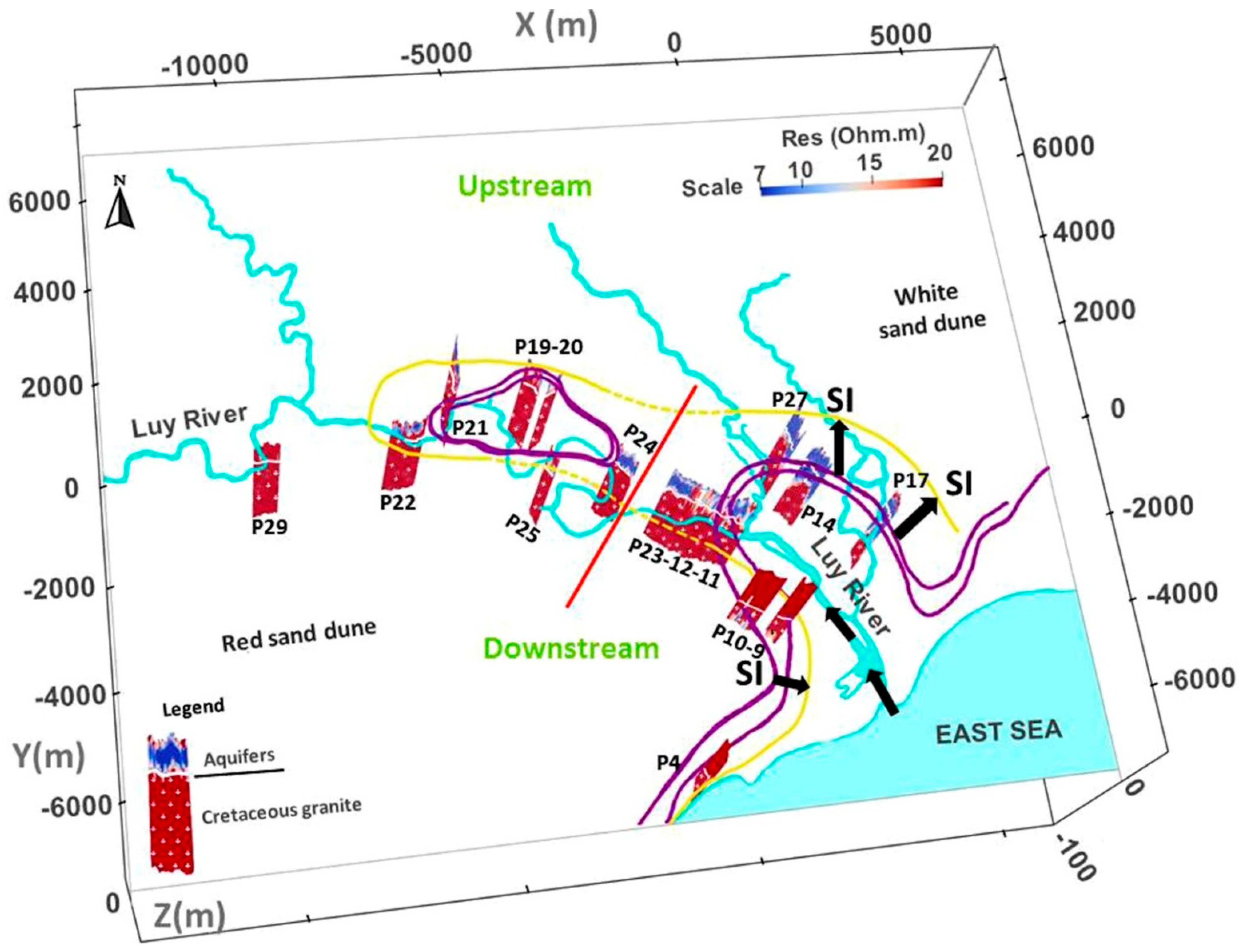
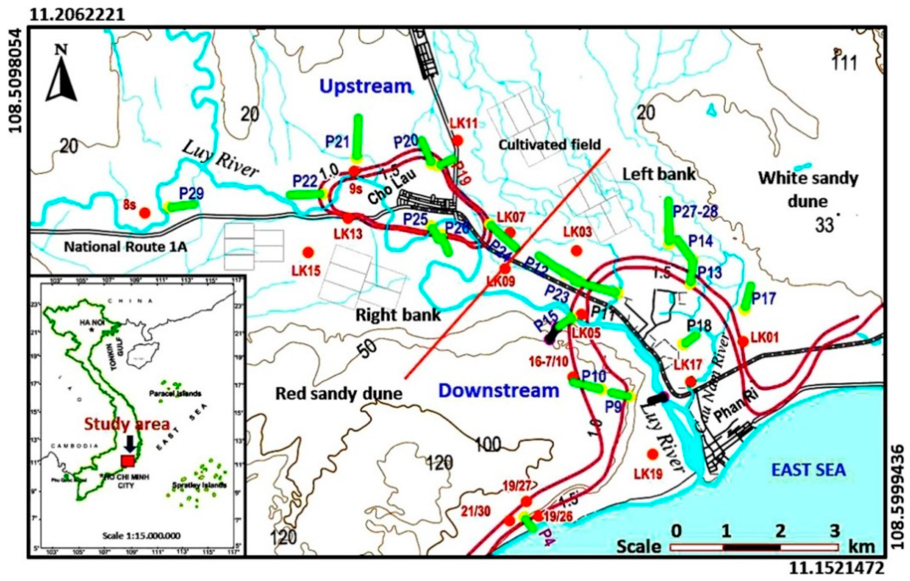
Understanding the dynamics of salt- and freshwater is thus essential but challenging for the management of the coastal aquifer [8]. Previous investigations mapped the transition of saline and freshwater into two different areas based on shallow boreholes in the downstream part of the Luy River. Two disconnected zones along the river were detected (Figure 1) so that the river was identified as the main source for SI [34]. However, a recent study estimated that seawater could penetrate about 7 km inland from the sea during the highest tide [35]. This could not explain the presence of saltwater as far as 15 km from the sea and the occurrence of several saline zones apparently disconnected from each other. The distribution of salinity is, therefore, more complex than expected.

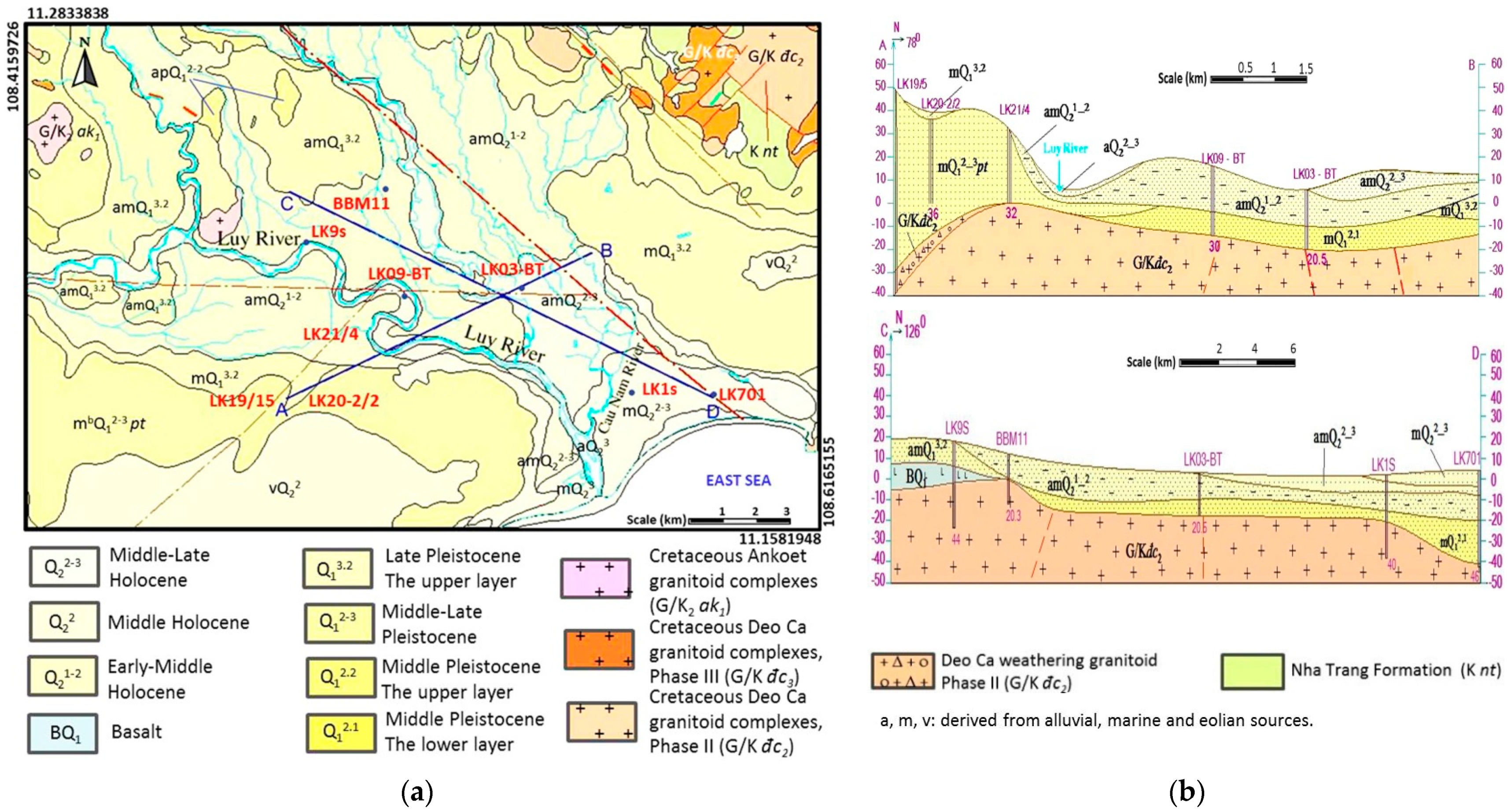
The alluvial plain of the downstream part of the Luy River is a part of the Binh Thuan coastal zone characterized by a U-shaped cross section and relatively homogeneous topography inclining gently toward the sea [31,36]. The study area has been governed by a part of the Mesozoic continental active margin commonly called Da Lat Zone [36]. This is proven by geological evidence consisting of the calc-alkaline magmatic arcs developed during the late Jurassic–late Cretaceous, such as the Deo Ca complexes of I-type granitoids [36,37,38], the Ankoet complex sourced from a mixture of I and S-type granitoid [39], and the Nha Trang extrusive formation (K nt) [36,37,38,40] (Figure 2a). In the Mesozoic and Cenozoic, the study site was affected by two perpendicular normal fault systems of NW-SE and NE-SW strikes [16] and subparallel fault (Figure 2a). The NW-SE faults were considered to be active in the late Mesozoic and reactivated in the Cenozoic, creating the Holocene and Pleistocene coastal sediment plains and the Neogene–Quaternary sediment basins which partly or totally overlay the older geological formations. The NE-SW faults are related to Neogene–Quaternary basaltic eruptions that created the shorelines in the same direction as the fault strike [37].

Sandy dunes are widely distributed on the right bank of the Luy river and along the rest of the Binh Thuan coastal zone. They were formed by complex geodynamic systems changing over time and depended on tide regime and sediment supplies. Generally, coastal sand dunes and bars are part of the Phan Thiet formation (m^bQ₁²⁻³ pt) (Figure 2a) from the Pleistocene period originating from marine and marine-eolian depositional sources and the weathering alteration of older bedrocks [38,41]. The sediment sequences are characterized by ridges of sand composed mostly of quartz but bearing some heavy minerals such as ilmenite, zircon, anatase, rutile, pyroxene, and monazite [36].

On the left bank, the flat plains have a low topographical elevation, including tributaries of the Luy River [34,41]. The sediments originating from complex alluvial-marsh-marine depositional cycles during the Holocene and Pleistocene are narrowly distributed and adjacent to the white sandy dunes and low hills [42] (Figure 1 and Figure 2). The sediment sequence is characteristic of this depositional system with gritty sandy layers intercalated with sand-rich clay or thin clay lenses that can locally acts as impermeable and confining layers (Figure 2b). The mineralogical composition is made mainly of quartz, feldspar, mica, and small rocky fragments from the bedrocks, such as granite, basalt, rhyolite, and dacite. These Holocene and Pleistocene sediment sequences also correspond to the unconsolidated aquifers constituting the main groundwater resource in the area. The Holocene aquifers (Q₂¹⁻², Q₂², and Q₂²⁻³, Figure 2b) have a thickness varying from 2 m to 20 m on the left bank and increasing towards the sea [16,27,35]. However, they are considered to be totally or partly absent on the right bank because of strong erosion and uplift processes [16,34,42,43]. Inversely, the Pleistocene aquifers (Q₁², Q₁²⁻³, and Q₁^3.2, Figure 2b) have a low thickness on the left bank, while they are relatively thick within the sand dunes on the right bank. The recharge of the unconsolidated Holocene aquifer depends directly on the resources of surface and rainwater. The storage capacity is limited and often insufficient for irrigation [16,34,42]. From previous studies, the Holocene aquifer is expected to be mostly salinized by saltwater intrusion in the estuarial part and coastal low land. The soil layers have also been degraded and salinized by agricultural activity [16,32,42]. In contrast, the abundant storage capacity and productivity of the Pleistocene aquifer is proven by the pumping test [30,32,34,42] and is considered to play an important role in irrigation and industrial production activities. Depending on the presence or absence of clay layers and lenses, the Holocene and Pleistocene aquifers can be separated by a confining layer or lying on each other, in which case they cannot really be discriminated (see borehole description in Section 5). Because of the tectonic activities, the bedrock formations are locally fractured and can contain local aquifers; however, their capacity is limited.

3. Methodology

3.1. Data Acquisition

Based on the existing saline boundary (Figure 1) identified through water samples collected from shallow wells at a depth ranging from 3 m to 8 m [34], 21 ERT profiles were collected using an ABEM^® Terrameter LS. A multiple-gradient array [44] with a separation factor s = 8 and an electrode spacing parameter a = 1, 2, 3, 4, 5, 6 was used for all profiles. This multiple-gradient configuration was chosen to accommodate the high contact resistance observed in most profiles due to dry soil conditions while maintaining a good signal-to-noise ratio and a good compromise between vertical and lateral resolution [45]. The electrodes were buried and sprayed with saltwater to decrease the contact resistance. The maximum injected current was limited to 200 mA to accommodate the high contact resistance observed in most profiles due to these dry soil conditions.

Each profile was originally composed of 64 electrodes but was extended afterward using the roll-along principle when possible [46]. An electrode spacing of 5 m was used to image the whole thickness of the unconsolidated aquifers with sufficient resolution (see Section 3.4 and Section 5.3).

3.2. Data Quality

The recorded raw data were first analyzed for their error level. Data quality was assessed using the contact resistance of the electrodes and the repeatability error. The latter was obtained by repeating the same measurement sequence and observing the coefficient of variation (expressed in %). All points with a coefficient of variation higher than 1% were removed from the datasets prior to inversion. This threshold was chosen based on the overall quality of the data.

The data quality was also assessed using reciprocal error [7,47,48]. Due to field conditions, we focused on gathering one profile per day, and collecting reciprocal for long profiles was too time demanding. Therefore, we have reciprocal for 8 out of the 21 profiles. The reciprocal error is defined as

e_N/R = R_N − R_R

(1)

where R_N and R_R are the normal and reciprocal resistance values, respectively. Slater et al. [47] proposed an error model where this error increases linearly with the mean R of normal and reciprocal resistances:

e_N/R = a + bR

(2)

where a represents the minimum absolute error, and b defines the relative increase of the error with the resistance. These parameters are determined by the envelope in an error versus resistance plot that contains all the points after the removal of outliers.

Globally, the reciprocal error confirms high data quality. Except for a few outliers, most data points have a relative reciprocal error $\frac{e}{R}$ lower than 5%, with the vast majority even showing an error below 1% (Figure 3a).

Following the methodology of Slater et al. [47], we investigated if a relationship exists between the error and the mean resistance (Figure 3b). For most of the profiles, no increase of the reciprocal error with the resistance is observed. Globally, the reciprocal error ranges between 0 and 0.001 Ohm, with similar values observed for the whole range of measured resistance. Fitting the envelope error model of Slater et al. [47] therefore results in a very low relative error (<1%) and an absolute error in the order of magnitude of 0.001 Ohm. A constant error model would actually be suited in this case.

3.3. Inversion

To recover the electrical resistivity distribution $\mathit{m}$ from the collected resistance data $\mathit{d}$, an inverse problem must be solved. In ERT, $\mathit{m}$ and $\mathit{d}$ typically cover several orders of magnitude and are often expressed in a log scale ensuring the positivity of the recovered resistivity. From a distribution of electrical resistivity, the corresponding dataset can be computed by solving the nonlinear forward problem noted:

$$\mathit{d}=f\left(\mathit{m}\right)$$

(3)

where f is the forward model operator.

The inverse problem is solved using a regularization approach, during which we minimize an objective function of the form:

$$\psi \left(\mathit{m}\right)=\psi \left(\mathit{d}\right)+\lambda \psi \left(\mathit{m}\right)$$

(4)

where the first term on the right-hand side of the equation expresses the data misfit, the second term represents the model functional with some assumed characteristic of the model, and λ, the regularization parameter, balances these two terms. The second term stabilizes the inversion process, in the sense that the sought model must verify some a priori properties [49].

This objective function can also be expressed as

$$\psi \left(\mathit{m}\right)={\Vert W_d\left(\mathit{d}-f\left(\mathit{m}\right)\right)\Vert }_p+\lambda {\Vert W_m\mathit{m}\Vert }_{\mathit{p}}$$

(5)

where $W_d$ defines the data weighting matrix accounting for varying data quality; $W_m$ represents the model constraint matrix, often chosen as the roughness matrix, although other options exist [21]; and the suffix $p$ refers to the $L_p$ norm.

We use the software Res2Dinv [50] to retrieve the resistivity distribution of the subsurface explaining the collected data. The L1-norm is used on both the data to reduce the potential effect of outliers and on the model to favor sharp resistivity contrasts. The solution of the inverse problem is obtained by minimizing this objective function using an iterative Gauss–Newton scheme, starting with an initial model ${\mathit{m}}_{\mathbf{0}}$ taken as the average apparent resistivity in the data set [50].

The topography is included in the finite-element mesh to avoid any undesirable effect of the surface on the recovered resistivity distribution. The topographical profile was extracted from the digital elevation model from the USGS (United States Geological Survey) and corrected with GPS data and field observations.

We considered that the inversion process converged once the data misfit reached a value below 3%, which was the case for all profiles. This is coherent with the error estimated from reciprocal measurements.

3.4. Depth of Investigation Index

ERT data collected from the subsurface are more sensitive to shallow layers than to deeper layers. The decrease of sensitivity and resolution with depth is well documented [51] and must be accounted for to avoid the overinterpretation of resistivity structures. This is even more crucial in saline grounds, as electrical flow lines tend to concentrate in high conductivity zones, which can significantly reduce the depth of investigation [8].

We follow the methodology of Oldenburg and Li [52] to calculate the depth of investigation index (DOI). The DOI is computed based on a dataset inverted with two different reference values (${\rho }_{ref1}$ and ${\rho }_{ref2}$) yielding two different inversion models (${\rho }_1$ and ${\rho }_2$) (Equation (6)). This is done by adding a reference model in the objective function (Equation (5)). ${\rho }_{ref1}$ and ${\rho }_{ref2}$ are generally chosen equal to 0.1 and 10 times the mean measured apparent resistivity in the data set.

$$\mathrm{DOI}=\left|\frac{{\log }_{10}{\rho }_1-{\log }_{10}{\rho }_2}{{\log }_{10}{\rho }_{ref1}-{\log }_{10}{\rho }_{ref2}}\right|$$

(6)

A low value of the DOI approaching zero indicates that the discrepancy of the inverted electrical resistivity between the two inversions is insignificant [52]. This is observed in well-resolved zones where the model is well constrained by the data. The inverted model is then considered to be reliable. Conversely, high values of the DOI approaching unity indicate that the inverted model is not well controlled by the data but rather by the regularization procedure (regularization and reference model). Those zones should be interpreted with caution. The DOI can be used to derive the maximum depth limit for which resistivity values are driven by the data rather than through the constraint of the reference model [52].

A threshold value is often used to delimit the reliable part of the profile. DOI values between 0.1 and 0.2 are often considered [52,53,54], but this threshold is rather subjective. More advanced methodologies have been proposed to objectify the choice of the threshold [55]. In this paper, we follow the proposal of Caterina et al. [51] to use the gradient in the DOI to define the threshold: when the DOI increases sharply with depth, it indicates that the role of the reference model becomes predominant in the inversion [51].

4. Petrophysics and Salinity Threshold

In porous sediments, the bulk electrical resistivity mostly depends on the resistivity of the pore fluid, the degree of saturation, and the presence of clay. The petrophysical relationship is classically expressed using Archie’s law [56,57]:

$$\frac{1}{{\rho }_b}={\sigma }_b=\frac{{\sigma }_f}{F}$$

(7)

where ${\rho }_b$ is the bulk electrical resistivity; ${\sigma }_b$ and ${\sigma }_f$ represent the bulk and fluid electrical conductivity, respectively; and $F$ refers to the formation factor, depending mostly on the porosity $\varphi$ and two empirical parameters: $m$, the cementation exponent, varying between 1 and 4, and $a$, an empirical constant close to 1:

$$F=\frac{a}{{\varphi }^m}$$

(8)

If clayey sediments are present, surface conduction related to the electrical double layer takes place and an additional term, the surface conductivity ${\sigma }_s$, which depends on the surface mobility of the ions in the electrical double layer and the excess surface charges taking part in surface conduction per pore volume unit, is needed in the petrophysical relationship [10]:

$${\sigma }_b=\frac{{\sigma }_f}{F}+{\sigma }_s$$

(9)

In the study area, the Holocene and Pleistocene aquifers are composed of a mixture of clayey and sandy sediments and are affected by the presence of saltwater. Both clay and salinity reduce the bulk electrical resistivity, and unequivocally interpreting low resistivity values as saltwater intrusions might be misleading.

Nevertheless, it should be noted that according to Equation (9), the effect of clay dominates the response when the fluid conductivity is low, i.e., in freshwater conditions. At high salinity, clay sediments only relatively contribute to the conductivity response, so that the lowest resistivity values can generally be linked to the presence of saltwater. Therefore, we use the following considerations in the interpretation of the resistivity profiles.

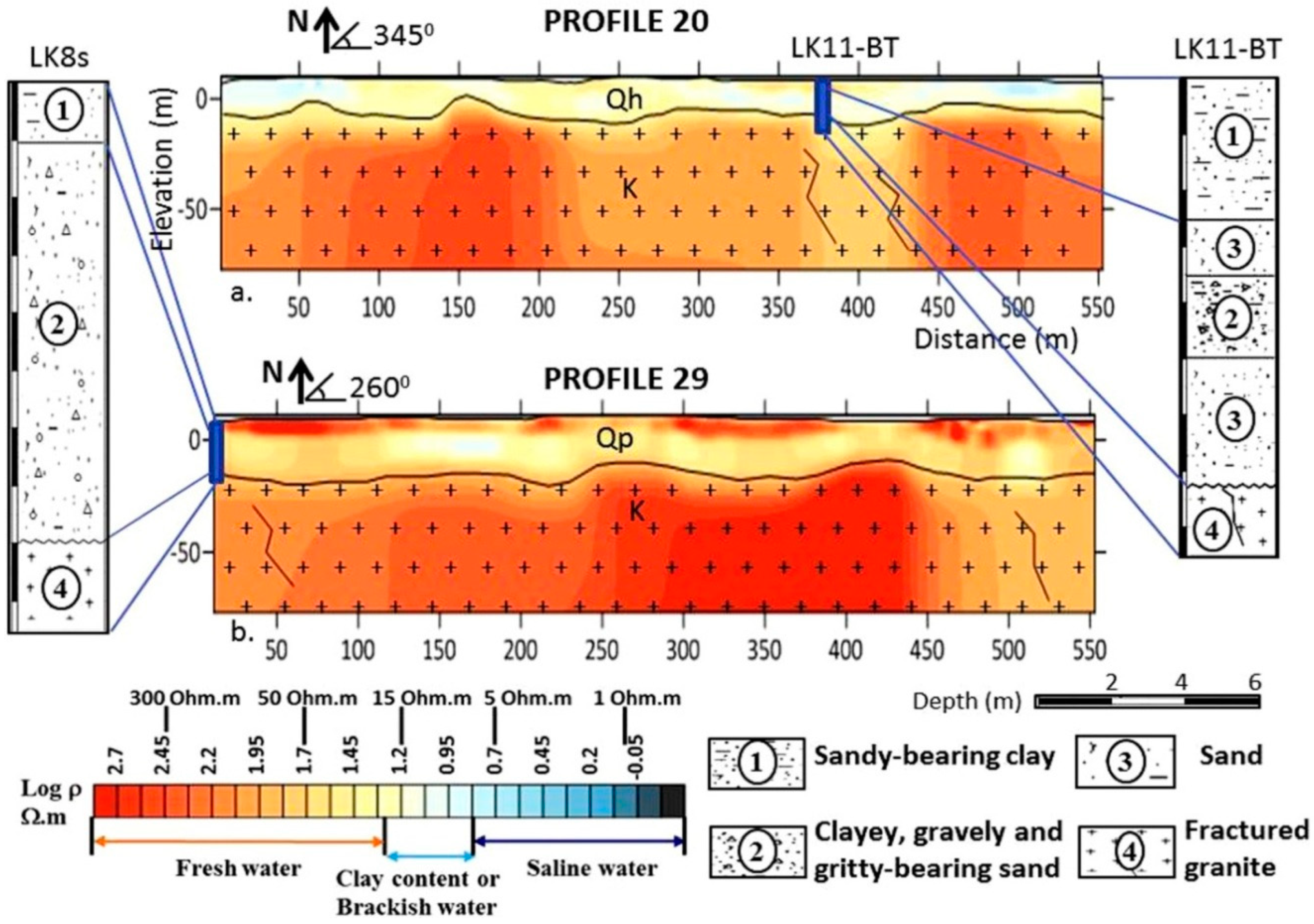
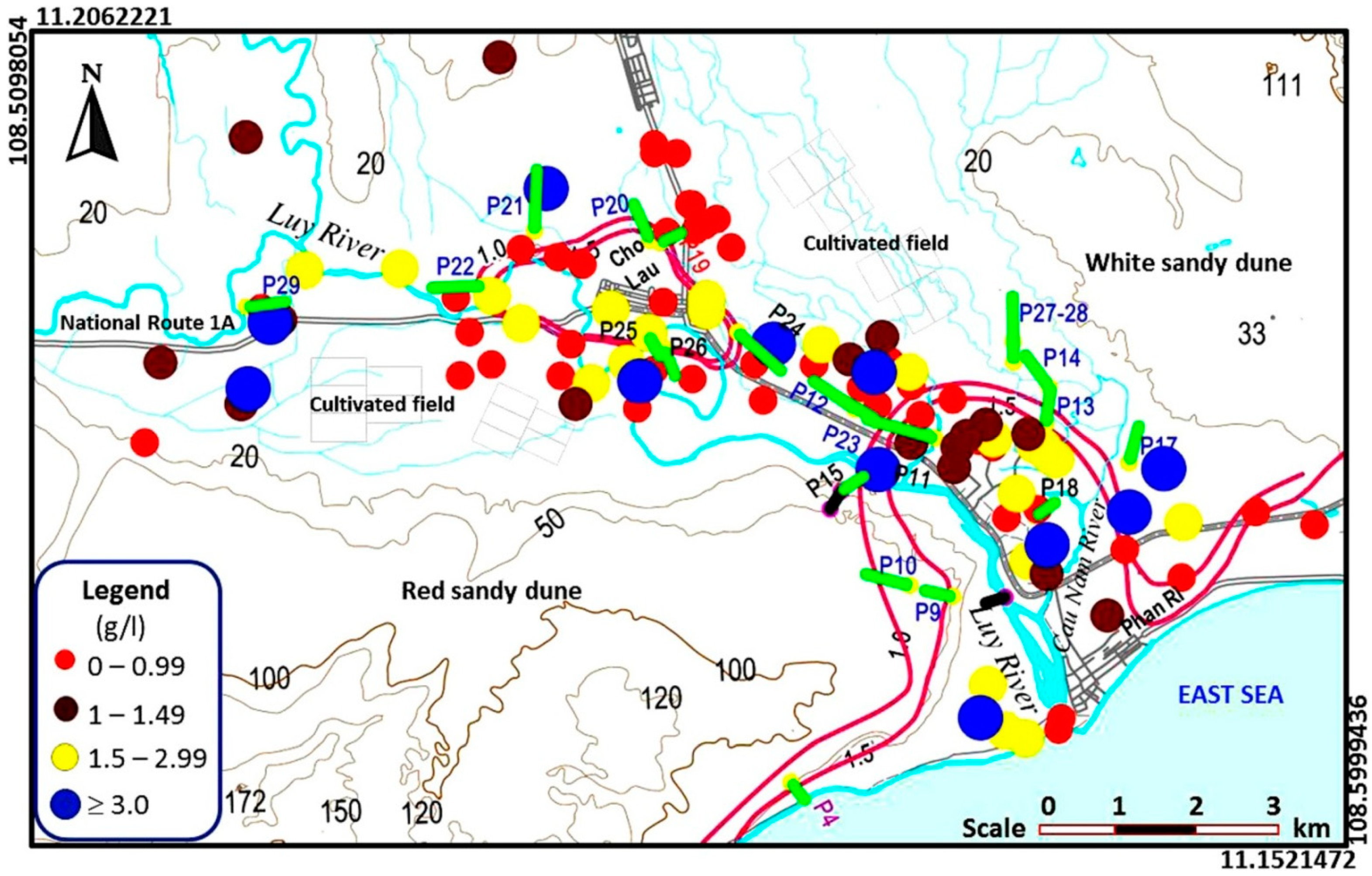
• Several profiles—for instance, 20 and 29 (Figure 4)—were collected in both freshwater conditions and clay-rich sediments as deduced from nearby water samples (Figure 5) and lithological descriptions of contiguous boreholes (e.g., Figure 4). On those profiles, the lowest inverted resistivity is in the range from 10 Ohm.m to 15 Ohm.m (Figure 4), which will be considered as the threshold for clayey sediments in freshwater conditions. Resistivity lower than the threshold will be considered as indicating the presence of salt or brackish water (Figure 5).
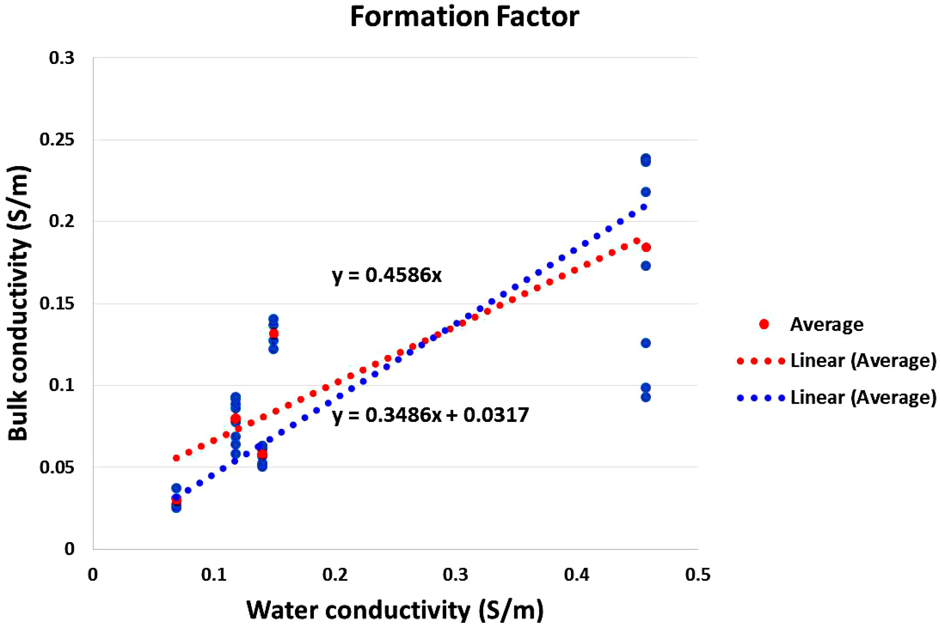
• The formation factor can be estimated using either colocated or laboratory measurements from Equation (7). Given the heterogeneity of the aquifer, the latter options would require collecting many samples and carrying out extensive laboratory experiments and bear the risk of the scale representability [14]. As an alternative, we identify the wells for which water samples were collected in close vicinity (but not colocated) of the ERT profiles, assuming that the observed salinity remains representative of the area. The well location was perpendicularly projected on the profile, and the bulk inverted resistivity at the corresponding depth was extracted. To account for the uncertainty of the projection, we extended the analysis to the neighborhood of the projected location in a range corresponding to the distance of the borehole to the profile.
• A fractional correction was also used for the temperature compensation, assuming that the increase of electrical conductivity is 0.02 °C⁻¹, in order to compare the conductivity at the reference temperature of 25 °C [58,59,60]. The temperature of the groundwater at the time of the survey was 30 °C.
• A linear regression (Figure 6) shows that an average formation factor from 2.2 (Equation (7)) to 2.8 (Equation (9)) explains the observed trend, consistent with values typically observed in sandy sediments.

Based on those considerations, it is now possible to estimate a resistivity threshold for the saline boundary. Based on the fluid electrical conductivity measured on the water samples (Figure 5), we approximate the relationship between fluid electrical conductivity (in S/m) and total dissolved solid content (TDS in mg/L) as linear, with ${\sigma }_f\approx \frac{TDS}{\alpha }$ [61]. The conversion factor $\alpha$ is commonly estimated between 5000 and 6500 [61]. The electrical resistivity of water at total dissolved solids (TDS) of 3 g/L, interpreted as the saltwater transition, would correspond approximately to 1.6 Ohm.m in the former case and 2.2 Ohm.m in the latter. Considering a formation factor between 2.2 and 2.8, the corresponding bulk electrical resistivity should be comprised of between 3.5 Ohm.m and 6 Ohm.m. Note that we used Archie’s law for the conversion, as the estimation of the surface conductivity from a limited number of points is inaccurate and its role for high salinity is limited.

According to these considerations, we can qualitatively interpret a resistivity value below 12 Ohm.m as characteristic of brackish (more than 1.5 g/L) to saline water. Similarly, resistivity values over 15 to 20 Ohm.m are indicative of freshwater (see color scale of Figure 4). To account for possible error in the estimation of the conversion factor and in the formation factor, we set our limit for the saline boundary (3 g/L) at a conservative limit of 7 Ohm.m.

Note that the actual threshold does not significantly affect the interpretation. The uncertainty related to our petrophysical analysis (in the range of 2 Ohm.m) is low compared to the uncertainty resulting from the inversion. Inverted resistivity values commonly overestimate the actual resistivity in saline conditions [6,18] but might enlarge the footprint of the low resistivity zone because of smoothing occurring during the regularized inversion process. Using conservative thresholds with a grey zone corresponding to resistivity in the range of 7 to 20 Ohm.m allows us to define saline and freshwater zones in a robust way.

In the next section, we use a unique color scale to display all the ERT results across the study area (Figure 4). According to the above considerations and related uncertainty, we chose a conservative threshold resistivity value of 7 Ohm.m to characterize the saltwater transition, with saline water occurring in blue areas with a resistivity lower than 7 Ohm.m. Freshwater is present in light yellow-brown areas with a resistivity higher than approximately 20 Ohm.m. Brackish water is found in the medium color areas ranging between bright yellow and bright light blue. Note that this range of value can also be characteristic of the presence of clayey sediments in fresh conditions and is thus the most difficult to interpret.

5. Results and Discussion

Considering the different topographical and sedimentary features, we divide our study site into two regions, namely the upstream and downstream parts. The limit between the two zones is chosen at a distance from the sea of about 7.5 to 8 km (Figure 1). This distance corresponds to the upstream saltwater intrusion limit in the river estuary during high tide [35]. The vertical axis on the figure always refers to the elevation expressed in m above sea level. Note that according to our thresholds, the term saline water will be used for resistivity below 7 Ohm.m. Brackish and freshwater correspond to higher resistivity values. Except if specified otherwise, these terms do not correspond to the salinity measured in water samples; they are simply used to ease the interpretation.

5.1. Upstream Zone

The upstream part is composed of eight profiles placed on cultivated fields with an alternation of dragon fruit and rice plantations (Figure 1), lying on the complex mixture of alluvial-marsh-marine alluvial deposits from the Holocene.

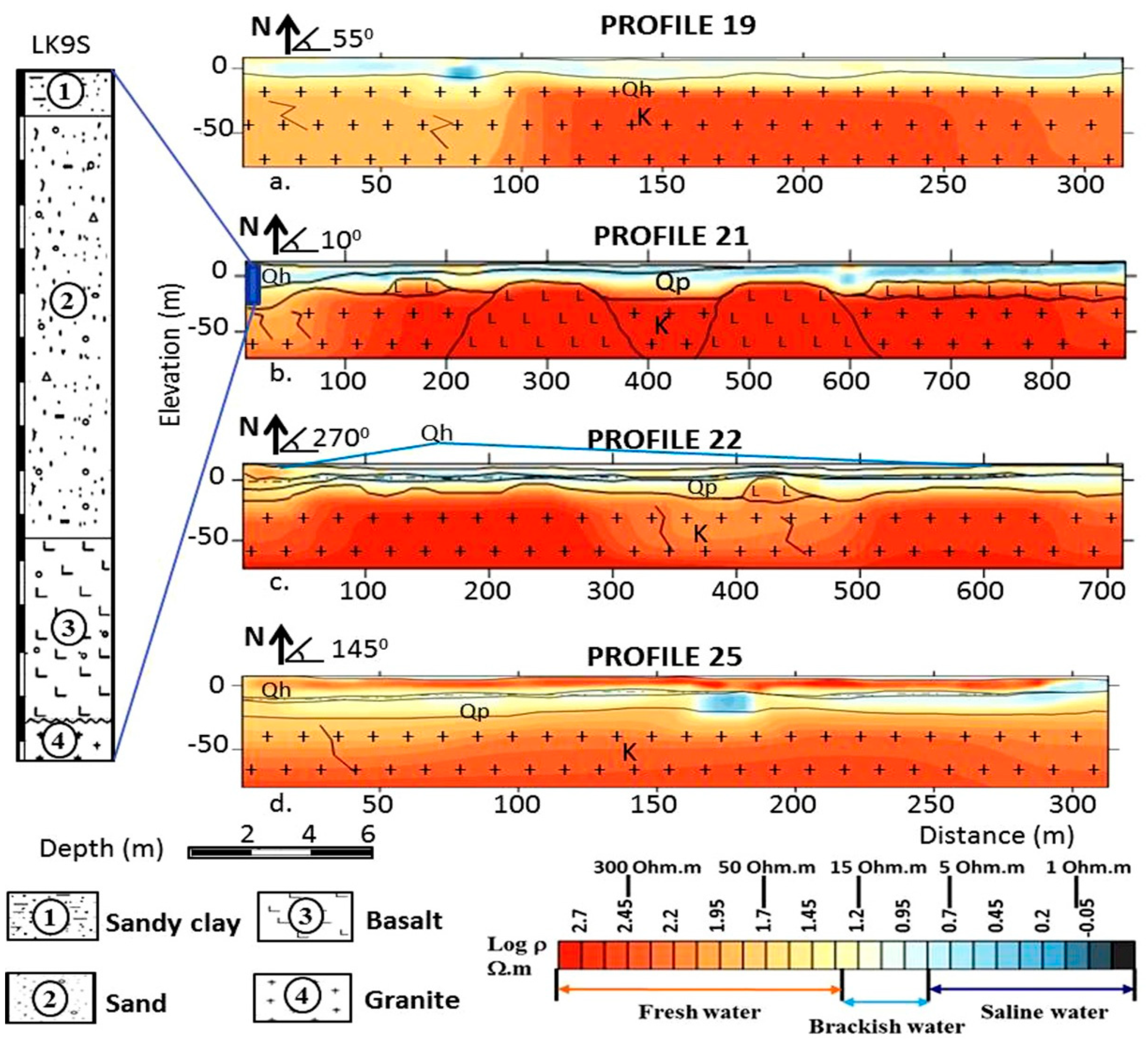
Figure 7 shows the inverted results of four profiles in the upstream part. The distribution of saltwater ($\rho$ < 7 Ohm.m) is discontinuous and seems to be limited to localized areas, as can be seen in profiles 19 and 22. The variation of resistivity values ranging from 1 Ohm.m to 7 Ohm.m at shallow depths indicates that saline water dominates the major part of profile 21. Brackish to fresher water lenses are commonly observed near the surface, characterized by higher resistive features above 10 Ohm.m. In this area, saline and brackish water seem to occupy mostly areas with low elevation along the Luy River. In the areas with slightly higher elevation, the lateral variation of resistivity features ranges from 10 Ohm.m to 20 Ohm.m, likely indicating that freshwater is dominantly present as observed in profile 20 (Figure 4), where clay lenses are probably responsible for the intermediate resistivity values. Profile 25 is adjacent to the river with the end of the profile corresponding to the river bank. Here, the intermediate range of resistivity might not only relate to clayey deposits but also point towards brackish water resulting from the direct interaction between the river and the aquifer. However, according to recent investigations, the part of the river directly affected by seawater intrusions during high tides would be limited to the downstream part [28]. This observation would rule out recent infiltration from the river to explain a higher salinity. Nevertheless, shallow water samples have revealed strong salinity variations at a small scale as well as the presence of saltwater in the vicinity of profiles 21 and 25 and further upstream (Figure 5). This is in accordance with our ERT profiles that indicate the presence of saline-water lenses within an almost fresh aquifer.

A reasonable assumption for this distribution could be the remnants of a past transgressive systems tract (TST) having taken place during the Pleistocene and Holocene [42,62,63]. Although these saline-water lenses would be expected to freshen with time through natural recharge, those processes could be slowed down in clay-rich layers in limited recharge conditions as observed in this arid region. The role of heterogeneity could explain the apparently discontinuous distribution of saline water in the aquifer of the upstream part. However, this should be confirmed by further investigations.

The sharp vertical variation of resistivity at depth indicates the transition to the underlying rock basement. This transition occurs at different elevations varying significantly from −10 to −30 m. As will be demonstrated in Section 5.3, this part of the profile is still located in the resolved part of the tomogram. Inhomogeneous structures are observed in the granite bedrock with resistivity values reaching from 500 Ohm.m to 1000 Ohm.m (Figure 7c,d). The transition between the unconsolidated layer and the bedrock is smooth, but this could be an effect of inversion, even if a blocky model constraint (L1-norm) was used to generate sharp contrasts during inversion. This could also correspond to a weathered zone in the upper part of the fresh bedrock. By comparison with the limited boreholes reaching the bedrock in the area, it was estimated that the depth of the bedrock was best corresponding with the 35-Ohm.m resistivity isoline.

As can be seen, the bedrock limit is not horizontal and displays lateral variations in the bulk resistivity. By combining it with borehole logs in the area [34], several specific features in the inversion results located in the basement are considered to correspond to small blocks of younger basement related to past magmatic activity (Figure 7b,c) [36,39]. We hypothesize that basaltic fluids erupted and penetrated through the older granitic bedrock that could be deformed and cracked. These assumptions are coherent with the presence of basaltic fragments observed in the nearby borehole LK15-BT and a basaltic bedrock layer overlying the granite in borehole LK9S (Figure 1 and Figure 7), located at approximately 2 km and 700 m of the profiles, respectively. Lower resistivity values ranging from 30 Ohm.m to 100 Ohm.m in the bedrock might be related to the increase of secondary porosity through fractures and the presence of secondary clay minerals originating from the weathering of the granite bedrock. Both features were also observed in boreholes.

5.2. Downstream Zone

In the downstream part, the flat plains at low elevations on the left bank of the Luy River are inclined toward the sea, with a slope ranging from 0 to 5° [31,43]. Seawater can intrude along the river in high tide conditions which can directly impact the aquifers. Nine ERT profiles were collected on the left bank, with five of them being in the direct vicinity (<700 m) of the Luy River or its tributaries. 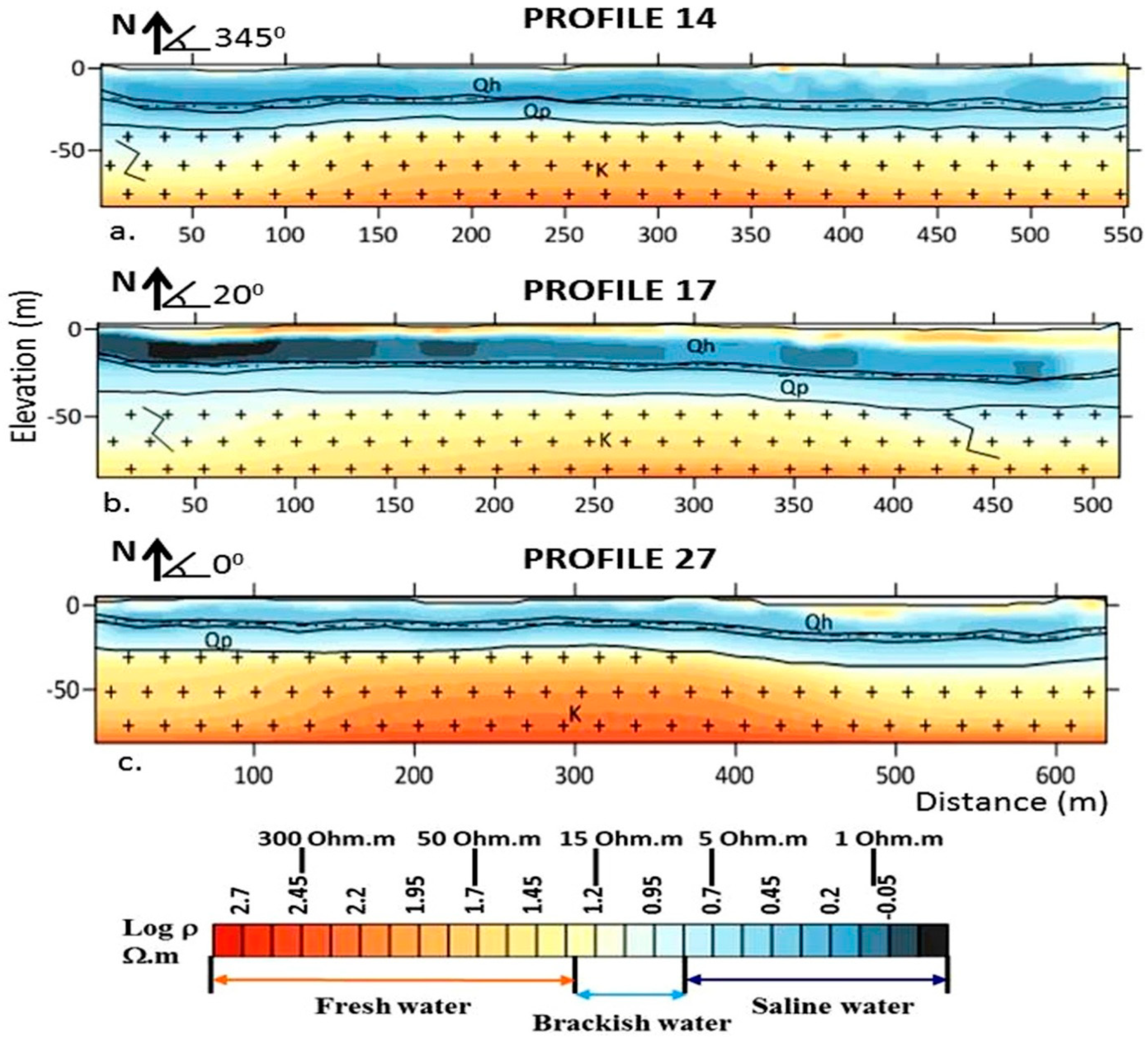Figure 8 shows extremely low resistivity in all profiles, fluctuating between 0.5 and 5 Ohm.m, which points towards the presence of high salinity values. Higher resistivity values varying from 7 Ohm.m to 35 Ohm.m are locally found near the surface. Saline water thus mostly occupies both the Holocene and Pleistocene unconsolidated aquifers. Freshwater is only present in lenses (Profile 27) or a thin layer (Profile 17) near the surface and is probably directly controlled by the infiltration of rainwater. In comparison with Figure 1, where the previously estimated saltwater boundary is depicted, the extent of saltwater migration into the aquifers seems to expand to the northeast and the north on the left bank of the river. Moreover, extremely high salinity is locally observed and indicated by a bulk resistivity lower than 1 Ohm.m in profile 17 (Figure 8b), which is close to a tributary of the Luy River (Cau Nam River, Figure 1). According to the petrophysical relationship, such a low value indicates a salinity close to that of seawater.

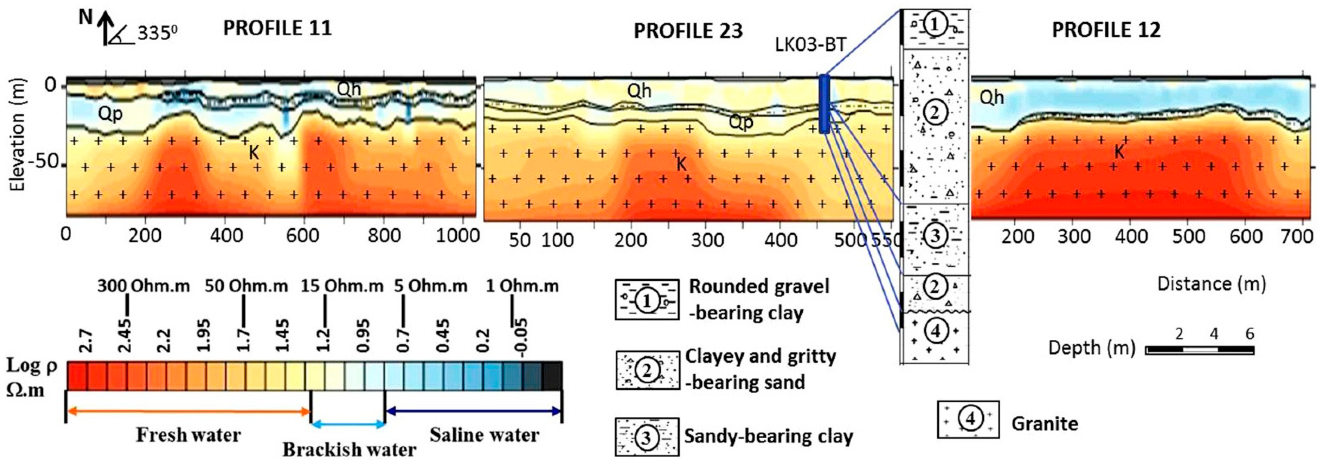
Closer to the Luy River, the succession of three profiles (namely 11, 23, and 12; Figure 9) also shows a complex distribution of salinity similar to that observed in the upstream part. Profiles 11 and 12 bear saline to brackish water with resistivity ranging from 1 Ohm.m to 10 Ohm.m. In contrast, profile 23 seems to have brackish to fresh water conditions as demonstrated by higher resistivity values fluctuating between 10 Ohm.m to 30 Ohm.m. This further illustrates that the fresh–saline conditions can vary rapidly within the aquifer. The salinity measured in shallow boreholes also visibly depicts this complexity in the fresh and saline water distribution (Figure 5).

As for the upstream zone, the transition to the underlying granite basement is well imaged by an increase in resistivity at an elevation of around −20 to −30 m. Lateral variations of electrical resistivity illustrate the heterogeneous structures of this granite bedrock, which is likely related to fractures and alterations. In Figure 8c, the resistivity in the basement reaches 500 Ohm.m, possibly indicating unaltered granite [64,65,66]. Inversely, quite low resistivity ranging between 10 Ohm.m and 30 Ohm.m is observed in the upper part of the bedrock. We assume that the electrical resistivity decrease of the bedrock indicates the presence of secondary clay formed during weathering processes. The unexpected low resistivity locally observed in the bedrock could point towards the presence of saline water that would have infiltrated from the unconsolidated aquifers through the hydraulically conductive fractures of the basement due to the density effect. However, these hypotheses could only be confirmed with direct observations.

On the right bank of the river, the sandy dunes correspond to a high elevation zone (50 m to 170 m above sea level, Figure 5). In the upper part of these deposits, high electrical resistivity values up to 5000 Ohm.m are imaged (Figure 10), indicating unsaturated conditions. At a larger depth, lower resistivity features ranging between 50 Ohm.m to 350 Ohm.m show that the remnants of the Holocene aquifer and the upper part of the Pleistocene aquifer are filled with freshwater. Deeper, the underlying Pleistocene aquifer contains cleaner and finer sands, probably in a more compacted state [67]. It is characterized by a sharp variation in resistivity ranging from 280 Ohm.m to 800 Ohm.m (Figure 10a). At an elevation of around −10 m, the electrical resistivity decreases significantly to a minimum value of 10 Ohm.m (Figure 10a,c). This elevation corresponds to the depth of the bedrock. We hypothesize that the top of the basement is either composed of clay-rich minerals in a strongly weathered condition or filled with saline water. However, the resolution in this zone is not sufficient, as the bedrock is located deeper below the surface compared to other investigated zones (see Section 5.3).

The dune area constitutes an important freshwater lens larger than 50-m thick, as observed in profiles 4, 9, and 10 (Figure 10). As it constitutes a preferential recharge zone, a freshwater lens has developed in the dunes and creates a natural hydraulic gradient towards the river and the sea. This possibly explains why less occurrence of saline water is observed on the right bank. It also seems to prevent the direct intrusion of saltwater from the sea, as illustrated in profile 4. The boundary of the saline–fresh interface is thus close to the sea on the right bank.

5.3. Depth of Investigation

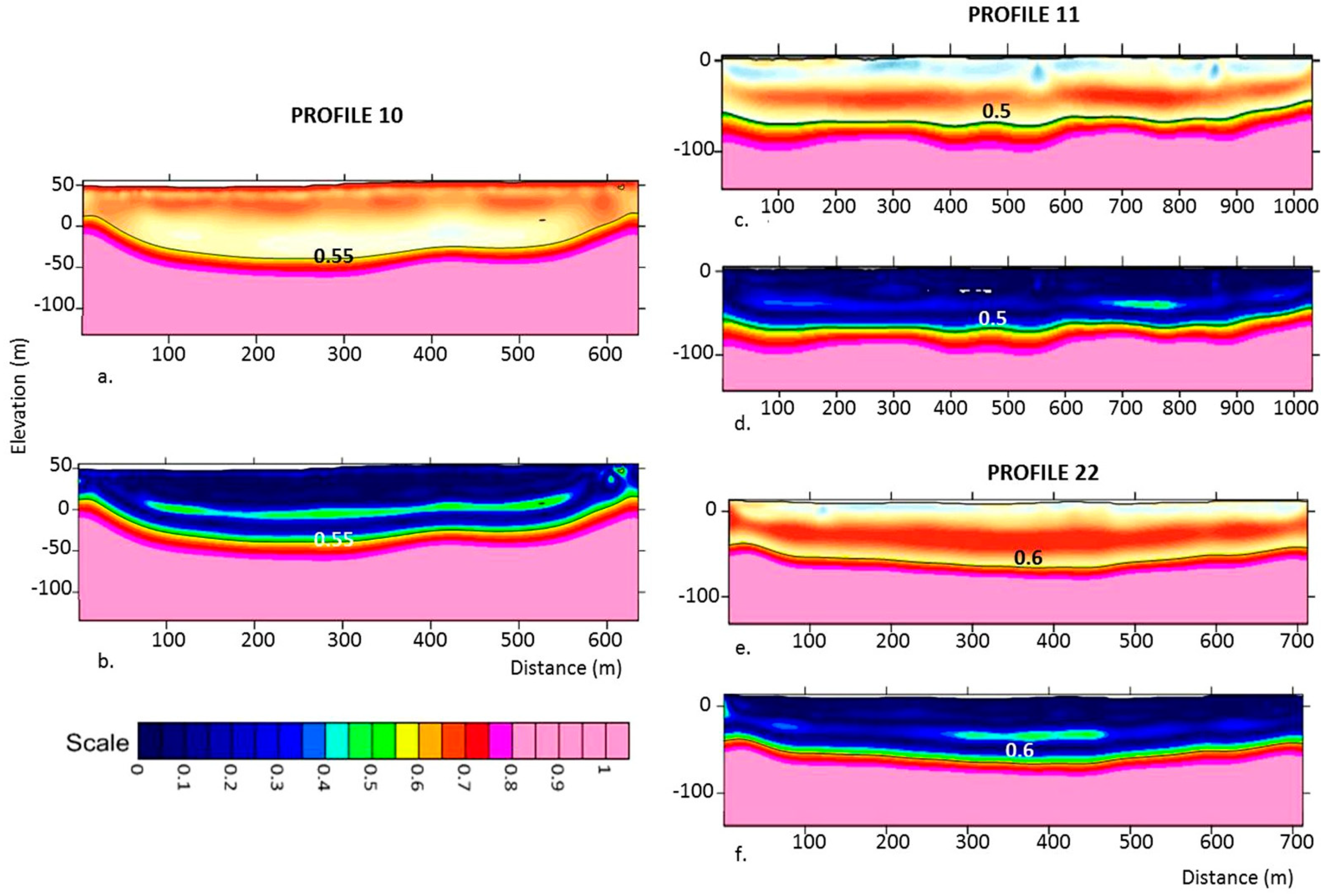
Figure 11 shows the DOI for one representative profile in each of the identified zones, as other profiles within the same zone show similar patterns. The DOI maps show the expected patterns, with the DOI approaching zero close to the surface down to about 35 to 50 m below the surface. At this depth, a zone with intermediate DOI values (0.2 to 0.4) visibly indicates that the two inversion models have slight discrepancies. For profiles in the upstream zone and on the left bank of the downstream zone (profiles 11 and 22), these zones correspond to the more resistive conditions of the bedrock. Typically, higher resistivity values are less well resolved, as current lines flow preferentially in conductive media. Therefore, the bedrock is well constrained as a resistive body, but its actual resistivity is uncertain. This is confirmed by the fact that the DOI increases sharply only at a larger depth between 75 and 85 m, which we consider as our threshold for determining the maximum depth of investigation. The same is observed in the right bank (profile 10), but the higher DOI values correspond to the depth of the transition to the bedrock. Below this limit, the results are not well constrained by the data. Therefore, both the unconsolidated aquifer and the upper part of the bedrock are located in well-resolved areas and can be interpreted, except on the right bank where the bedrock depth corresponds to a higher DOI, indicating that interpretation of the bedrock should be made with caution, although the decrease in resistivity itself seems consistent in all representative profiles.

5.4. Advantages and Limitations of the Methodology

In this paper, we have tackled the challenging task of interpreting ERT data in terms of salinity with sparse colocated data. As with any attempts to quantitatively interpret ERT results, our methodology suffers from limitations that are discussed below.

As can be seen from Figure 5, the estimation of the formation factor is limited by the amount of available data. Because of the absence of colocated data, we had to consider the uncertainty related to the distance between the ERT and wells, so that only five wells were considered sufficiently close, and a large spread of values is observed. Some points also deviate from the trend, likely indicating that a single petrophysical relationship might not be sufficient to characterize the study area, as expected from the heterogeneity of the sediments. On the one hand, it is clear that the methodology could benefit from a more robust estimation of the formation factor. On the other hand, the few available points are not only enough to validate the expected trend but also derive a formation factor coherent with values found in the literature.

It is well known that the bulk resistivity values obtained after inversion can deviate strongly from the real bulk resistivity values. If advanced methodologies incorporating prior information can help to reduce the discrepancy, these often require additional data. It is clear that low resistivity values are likely overestimated, high resistivity values are underestimated, and the transition zone might be an effect of smoothing rather than the truth. This can obviously alter the interpretation of ERT images.

Nevertheless, our methodology allows addressing both limitations. Using a conservative limit for the saline and fresh boundaries, we limit ourselves to a semiquantitative interpretation (saline, brackish, fresh), but we avoid introducing errors in the interpretation. Indeed, the choice of the thresholds was conservative to avoid the influence of errors made in the petrophysical relationship and left a “grey zone” between saline and fresh classes, accounting for the likely presence of clay lenses in the study area, which is difficult to discriminate from brackish water. The interpretation in terms of boundaries is still relevant, as the difference between 5 and 10 g/L makes little difference for farmers: in any case, the water is above the useful limit. It also allows integrating geophysical data in conceptual hydrogeological models or even more broadly in the calibration of numerical models.

In addition, the systematic use of the DOI map allows limiting the interpretation to reliable zones within the inverted images. In our case, it allows results down to a depth reaching 80 m to be interpreted, which is sufficient for the characterization of unconsolidated sediments.

The complete ERT inversion models produce a quite clear overview of the link between the bulk resistivity values and both the stratigraphic units, especially of the bedrock, and the salinity.

6. The New Fresh–Saline Groundwater Map

The ERT results are used to update the previous saline boundary map from NAWAPI [34]. In Figure 12, we summarized every ERT profile as a two-layer log displaying the average resistivity value of the aquifer and the bedrock as well as the depth of the bedrock. The blue scale indicates the salinity in the unconsolidated sediments, while the red corresponds to freshwater conditions. The boundary (yellow solid line) corresponds to our interpretation based on ERT, corresponding to an estimated TDS value of 3 g/L in the unconsolidated aquifers. Dotted segments indicate a lack of data to conclude with certainty. Local variations within the zones (presence of salt/fresh water lenses) are possible as described in Section 5. Note that the original map used a threshold of 1.5 g/L; the extension of 3 g/L based on shallow water samples would have been even more restricted.

Generally, the boundary of saline water expands toward the north and northeast up to at least 1.5 km compared to the initially mapped saltwater extension. This observation is mostly based on the profiles collected on the downstream part of the left bank of the river. The extension could even be larger as neither water samples nor ERT profiles were collected further in the north. On the right bank, our ERT profiles show that the dune area and its freshwater lens constitute a protection against SI, as the hydraulic head is larger and groundwater flow is directed towards the river and the sea. Therefore, the zone of saltwater intrusion is narrower in the southeast than previously estimated. If this zone could be seen as a freshwater reserve, SI could eventually occur if this lens was uncontrollably exploited.

The discrepancy with the previous map is probably related to the fact that ERT investigates the whole aquifer thickness, while the old map was based on shallow boreholes. Our ERT investigations show that a freshwater lens can exist on top of the saline water. This observation is also corroborated by the experience of farmers who exploit shallow wells and by our latest investigation during the period from 2020 to the first half of 2021, during which an increase in salinity was observed in the dry season because of overexploitation. An alternative solution would be to accumulate freshwater during the rainy season for consumption in the dry season.

In the upstream zone and part of the downstream zone, the distribution of saline water is extremely heterogeneous and complex as shown by both the high variability of salinity from water samples and ERT profiles at short distances. The presence of SI cannot be explained only by interaction with the river, as previously thought, but might also result from the interplay between past transgressions with connate saltwater filling the sediment pores. The presence of clay layers and lenses acting as flow barriers and trapping connate water, complicated recharge patterns influenced by the presence of clay near the surface, and agricultural practices including water extraction and irrigation could prevent freshening processes. This is further confirmed by the presence of saline water towards the western part of the river catchment (Figure 7), but no ERT profiles were collected in that zone.

The origin of saltwater is thus probably a complex combination of different processes. Recent intrusions related to the flow regime of the Luy River likely play a notable role in the downstream part, including along tributaries, where high tides in areas with low elevations can result in direct infiltration from the river into the aquifer. The uncontrolled exploitation of the aquifer for irrigation and industrial production can further accelerate the migration of saline water.

However, ERT data shed new light on the distribution of saltwater in the area. The presence of freshwater lenses of a limited extent on top of the more saline and deeper aquifer could indicate that the development of a freshwater aquifer, as expected from natural recharge, is slow and likely perturbed by human activities, namely water extraction and irrigation practices, aquaculture, and salt production leading to a depletion of these limited freshwater resources. Moreover, the complex distribution of saltwater, including in the upstream part of the catchment, far from the sea and the river, seems to indicate the presence of connate saltwater buried in the sediments that has not been freshened yet. These hypotheses cannot be resolved from ERT data only but require additional analysis, such as hydrochemistry and flow and transport modeling [68].

Moreover, saltwater intrusions could also reach deeper zones of the bedrock under the sea level. If the presence of saltwater in the basement in the downstream part of the river on both banks, including under the sand dunes, was confirmed, this would likely indicate that the origin of almost all the saltwater is related to past transgressions. Indeed, if freshening processes are expected, for example, under the dune areas, these can be impeded by low hydraulic conductivity zones slowing down groundwater flows, as could occur in fresh bedrock, weathered zones containing a significant content of secondary clay, or in clay sedimentary deposits. But this should be confirmed by direct borehole information, as the resolution of ERT at this depth is not sufficient to make an unequivocal conclusion.

7. Conclusions

In this paper, we developed a new methodology to interpret ERT data in terms of salinity in a heterogeneous aquifer in the absence of colocated data. We defined a conservative threshold of resistivity to interpret semiquantitatively saline and fresh boundaries.

We applied the methodology to the Luy River water catchment, Binh Thuan province, Vietnam. The estuaries of the rivers in Binh Thuan are assumed to be the key driver for saltwater intrusion along the coastal areas during high tides [28]. However, our investigation revealed that the zone affected by SI is much larger than previously expected from shallow water samples. In particular, the bottom part of the unconsolidated aquifer systematically bears saltwater on the left bank of the downstream part of the Luy River system. The high elevation dune complex constitutes a freshwater reserve that partly protects the right bank of the river from SI. ERT also reveals a complex distribution of SI in the upstream part of the river, falsifying the hypothesis that the river is the only driver for SI in the area. Other processes, including paleohydrological conditions, geological heterogeneity, and agricultural practices, likely play a preponderant role. We plan to build on this preliminary study to develop a numerical model of the aquifer, test the different hypotheses, and propose a sustainable management of the water resources.

As demonstrated in our study, ERT is a suitable tool to collect semiquantitative data on saline water intrusion, even in the absence of extensive colocated data for validation. It is cost effective and easy to apply both in rural and semiurban areas and should be generalized for the characterization of seawater intrusion in complex environments.