Article

Assessment of the Climatic Variability of the Kunhar River Basin, Pakistan

1
School of Water Conservancy Science and Engineering, Zhengzhou University, Zhengzhou 450001, China
2
Department of Technology, The University of Lahore, Lahore 54000, Pakistan
3
School of Civil, Mining, and Environment, University of Wollongong, Northfields Ave, Wollongong, NSW 2522, Australia
*
Author to whom correspondence should be addressed.
Water 2021, 13(13), 1740; https://doi.org/10.3390/w13131740
Submission received: 21 April 2021 / Revised: 14 June 2021 / Accepted: 16 June 2021 / Published: 23 June 2021
(This article belongs to the Section Hydrology)

Abstract

:
Pakistan is water stressed, and its water resources are vulnerable due to uncertain climatic changes. Uncertainties are inherent when it comes to the modeling of water resources. The predicted flow variation in the Kunhar River Basin was modeled using the statistically decreased high-resolution general circulation model (GCM) as an input for the Hydrologiska Byråns Vattenbalansavdelning (HBV) model to assess the hydrological response of the Kunhar River Basin under prevailing climate changes. The model’s best performance during the calibration and validation stages was obtained with a regular 0.87 and 0.79 Nash–Sutcliffe efficiency in the basin, respectively. Under the high-end emission scenario, a 122% increase was expected in evapotranspiration in the rising season of months during the winter period 2059–2079, and such developments were attributed to an immense increase in liquid precipitation and temperature. The model’s output reflects a potential for basin stream flow in terms of increasing liquid precipitation up to 182% at the beginning of the monsoon season in the period 2059–2079 in the scenario of high-end emissions. Moreover, the study produced possible uncertainties in high-elevation zones, where the modeling of a catchment can lead to typical snow ablation and accumulation in future projections. This study revealed that the precipitation rate will increase annually, resulting in an increase in the summer stream flow over the basin, though snow is hardly expected to accumulate in the basin’s future climate.

1. Introduction

Hydrological systems are considered to be excessively critical with respect to their direct effect on economic and environmental development. The hydrological cycle of a basin is greatly influenced by the basin’s physical features, climate, and human activity. Many researchers have found that temperature, precipitation, humidity, and wind trends are changing in climatic variables, particularly in precipitation and temperature [1,2]. In recent years, Taylor RG et al. (2013), Green TR et al. (2011), Goderniaux P et al. (2009), and Eckhardt et al. (2003) have initiated the use of general circulation models (GCMs) to investigate the consequences of future climate change on global water resources [3,4,5,6]. The spatial resolution (200–500 km) for models limits their application to being considered appropriate for the basic level; as such, an excellent spatial resolution is needed for small basins [7]. Researchers have developed complex, quantitative, and computationally efficient techniques for routing basin scales and GCM resolution. With a high resolution of 5–50 km, the regional climate model (RCM) uses the GCM’s efficiency while providing high-resolution quality and extensive data on the basin level. Quantitative equations for studying the basin scale and GCM (precipitation and temperature) were developed with statistical downscaling (SD) methods [8]. Statistical downscaling methods thus ensure that successful strategies/approaches are adopted by scientists. Ankur Srivastava et al. used the variable infiltration capacity (VIC-3L) semidistributive model to estimate evapotranspiration (ET) on a grid scale with satisfactory results over a tropical river basin in eastern India [9]. The author has, also on this river, successfully quantified its main hydrological components using the VIC-3L semidispersion model and the identification of unit hydrograph and component flows from the rainfall, evapotranspiration, and streamflow (IHACRES) conceptual model [10]. Another conceptual model, the satellite-based hydrological model (SHM), has been evaluated with positive results, but the scope has not been expanded as the product has not yet been developed outside India [11]. The HBV model is used in order to predict expected river water flows in these kinds of large and small basins [12,13].
In recent years, as a result of the general circulation models (GCMs), increasingly detailed, quantitative, and integrated prototypes have been incorporated with hydrological models to investigate future predictions of climate change in river systems in different regions of the globe [14,15,16]. These may not be appropriate at the watershed scale in specific smaller watersheds, which demand a fairly fine image quality [17,18]. Rainfall–runoff methodologies and mathematical modeling been established to link the precision of the GCM and the river scale. A wide-quality digital regional climate model (RCM) with a complicated downscale of approximately 5–50 km was used with the outcomes of a GCM to give details and high-quality river system outcomes [19,20]. Furthermore, statistical downscaling (SD) methods, e.g., climate prediction, correlation, and transcription of climatic conditions, produce empirical and statistical connections (e.g., temperatures and precipitation) between the GCM scale and the watershed-level parameters. In particular, in comparison to dynamic downscaling, SD techniques, which are computer based, are significantly faster, offering approaches that can be easily embraced by the broader scientific community [21].
Pakistan is one of the countries under the most stress due to reductions in its water resources from just 5000 cubic meters per capita in 1952 to 1100 cubic meters per capita in 2014 [22]. A United Nations study revealed that countries with fewer water sources, such as 1000 cubic meters per capita annually, are classified as having scarce water [23]. Thus, under rapidly changing climate conditions, an exact estimate of future water resources would greatly help in terms of operating, planning, and managing hydrological installations in Pakistan [24,25,26]. Various research, such as that of Akhtar et al. (2008), Bocchiola et al. (2011), and Ahmad et al. (2012), has evaluated the adverse effects of weather changes on Pakistan’s water resources [8,11,27]. Most of these studies were accomplished with hydrological modeling throughout the Upper Indus Basin, which used the snowmelt runoff (SRM), the SWAT, and the water and energy budget-based distributed hydrological model with improved snow physics (WEB-DHM-S) prototypes. Thus far, no studies have been conducted in the Kunhar River Basin with the HBV model. This basin is one of the major influences of the Jhelum River and is completely within Pakistan. The genetic impacts of climate change on water resource systems can be explored because the water that melts from the glacier significantly affects the flow of water in the Kunhar River Basin [28,29]. Precipitation rises whenever snow melts and then accumulates if melting ends [30].
In addition, in-depth studies on hydrology and the need to improve water resource management require a full awareness of the advantages and disadvantages of the GCMs that are popularly studied across different regions. Lumped conceptual models were thoroughly compared in order to determine the best performing model for reproducing different components of the hydrograph, including low and high flows in data-poor catchments [10,31]. In general, GCMs can be used as inputs in hydrological studies because of their uniform datasets, and these products can be used immediately in flow simulations. This is the great advantage of reanalysis datasets when comparing them to satellite precipitation products, which lack accompanying temperature data and heterogeneous timescales. To the best of our knowledge, the applicability of GCM data for hydrometeorological studies has not yet been adequately investigated outside of China, including in Southeast Asia [32]. The huge, rugged areas of hydrometeorology in Pakistan usually depend upon the geography; alpine terrain generally has significant amounts of solid and liquid rainfall, which can also be accumulated as reservoirs. This can serve as an incredible resource for climate crisis detection and climate impact assessment [33,34]. The complexity and mutual interdependence of environmental activities at high altitudes in nature produce massive issues in the investigation of the impact of the atmosphere [35]. Rapid river discharge forecasts through different climate change scenarios can provide significant guidance for monitoring national energy systems by providing timely alerts of extremely high or low discharge volumes, which would allow hydroelectric power to be adjusted by electrical power systems [36]. This paper predicts these initiatives because it provides appropriate statistics for developing effective strategies for Indigenous experts, which would ultimately contribute to water protection and sustainable development in the basin [37,38,39,40].
The study of projections of river modeling quickly gained attention in the context of climate change and environmental change [41], as have their combined impacts on water supplies and society. It is therefore important to consider the dynamics of the hydrological system in the Kunhar River watershed to predict the future stream flow. After recognizing the roles of the watershed’s various components (e.g., land use, soil, geology, snow, glaciers, and climate) in discharge, the relationships were identified. Consequently, annual freezing rainfall management and stream flow prediction in Pakistan’s snowy areas are of crucial significance, as water resource management is one of the major issues of the Kunhar River system. According to these conditions, the prediction of streamflow in the Kunhar River while considering climate is an important topic for discussion because it could help in terms of utilizing and managing water resources in the region [2]. The aims of this study were (1) to apply the HBV model in the Kunhar River while considering snow conditions and climatic concerns and (2) to determine the probability of fluctuation in river streams with the GCM. The core objective of this study is to predict the climatic behavior of the Kunhar River Basin for the period of 2017 to 2079.

2. Data and Methods

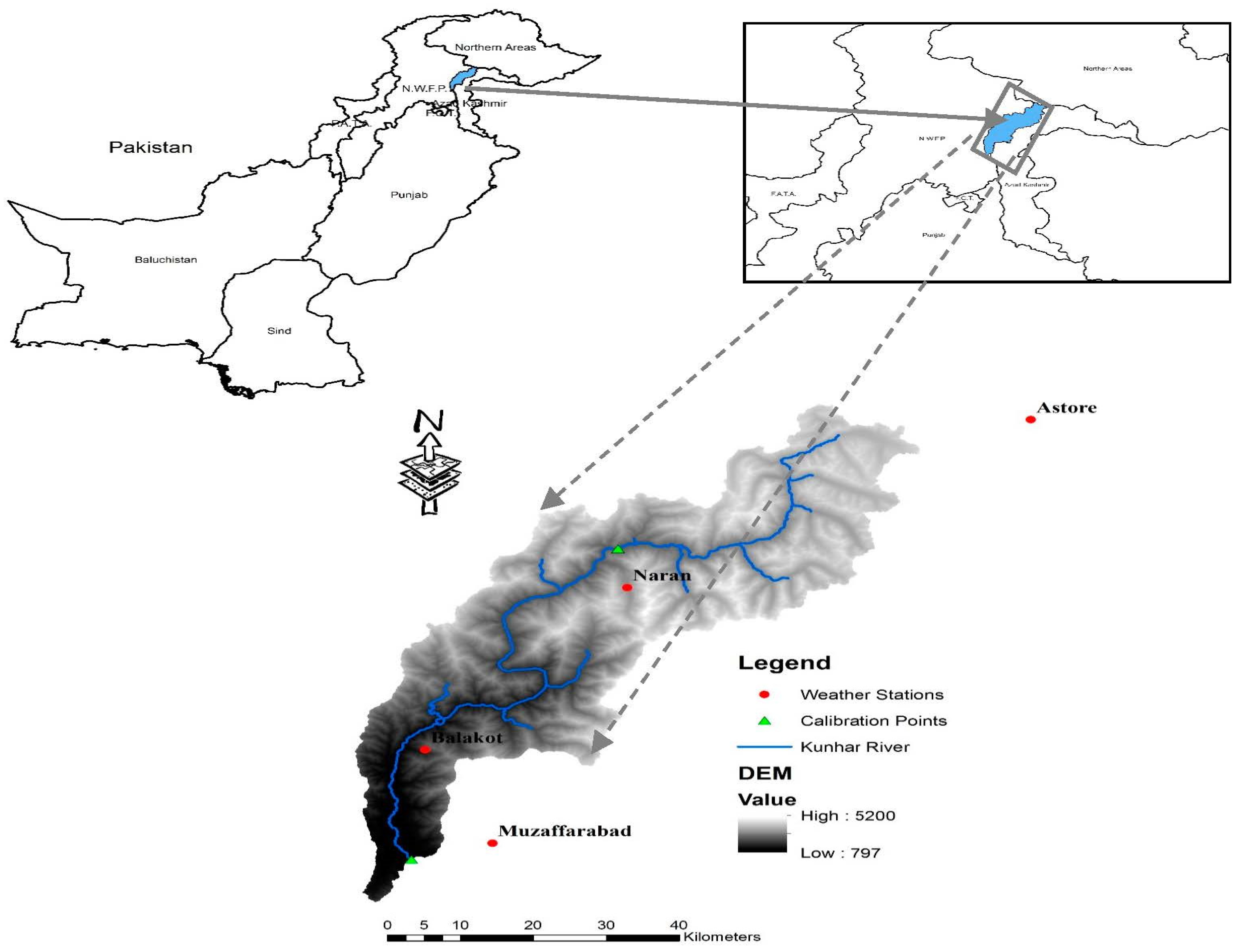
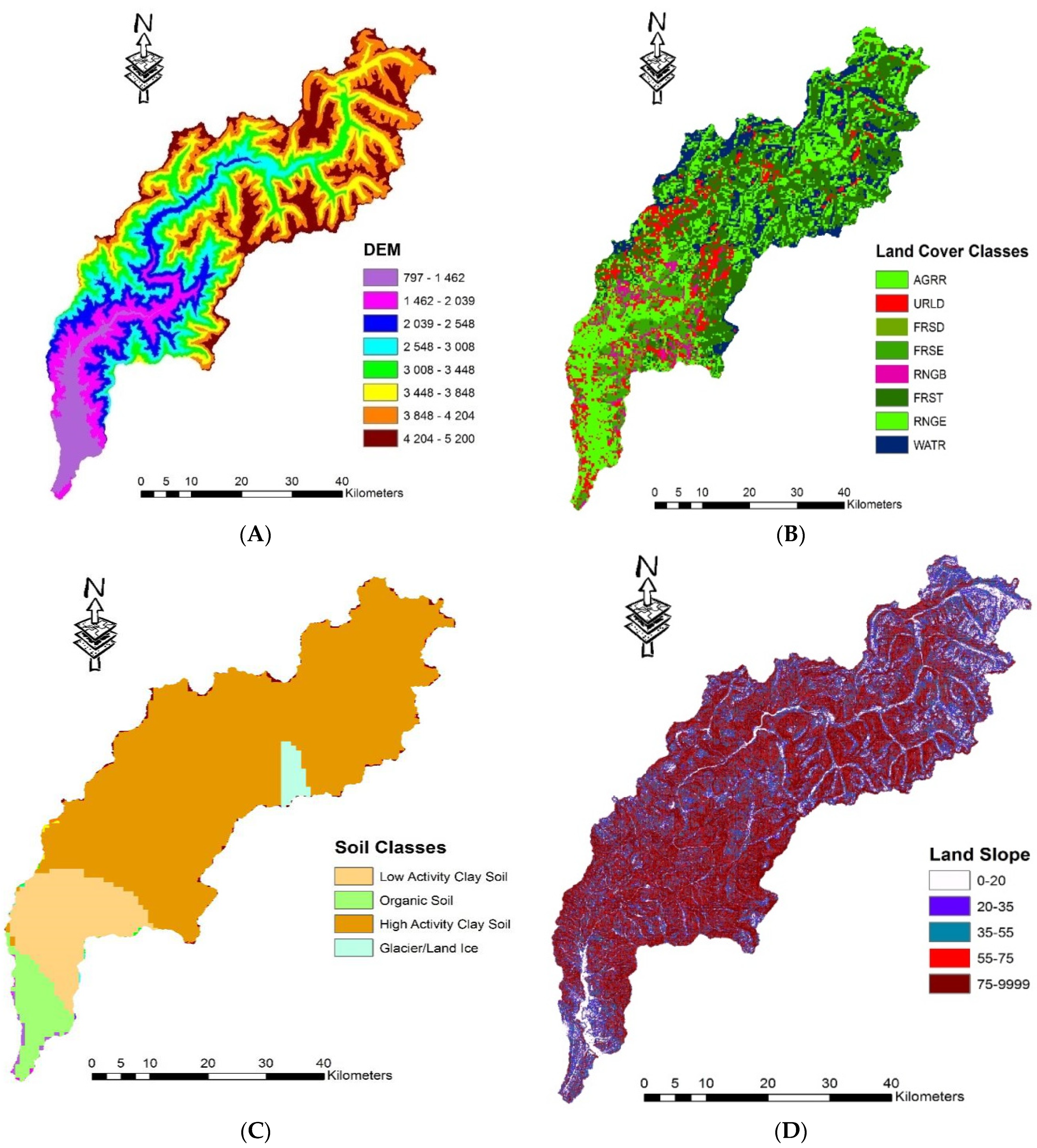
2.1. Study Area Description and Data Sources

2.1.1. Kunhar River Basin

The Kunhar River watershed is located in the northern part of Pakistan with the coordinates 34.2°–35.1° N, 73.3°–74.1° E (Figure 1). The Kunhar River flows through the southern plateau of the Greater Himalayas. It comes directly from the Kaghan Valley and through Lulusar Lake. It passes through Bata Kundi, Jalkhand, Kaghan, Naran, Balakot, Kawai, and Gari Habibullah, and it meets the Jhelum River at Rara [42]. As far as the water of Kunhar is concerned, it is rich in algal flora and thus harbors a great diversity of aquatic life. The drainage area possessed by the Kunhar River is 2535 km2, and the elevation ranges from 600 to 5000 m. The Kunhar is regarded as one of the transboundary area’s most significant tributaries [43]. Figure 2 demonstrates the more important topography, such as the contour lines, gradient, delineated sub-basins, and aspects obtained with DEM. This figure shows that the sloping intensity of the Kunhar River ranges from 0″ to 76″ km. The plateau along the Kunhar River is moderately sloped. It is crucial, however, to note that the majority of the basin is moderately sloped (>8° and 29°) [44]. The large variety of vegetation includes subtropical grassland forests, temperate grassland forests, agricultural land, high mountain glaciers, and snow [45,46]. This challenging topography was categorized into seven key classifications to investigate the Kunhar River Basin’s surfaces. Most of the area of the watershed is occupied by snow, agriculture, and forests. This knowledge was obtained from land coverage data from the Kunhar River Basin with a 1-km resolution.

2.1.2. Data

For the current study, climate model statistics (highest temperature, lowest temperature, and rainfall) were also acquired [47]. The SDSM (statistical downscaling model), a system composed of various systematic explanatory variables and meteorological data, was used with the worldwide weather patterns from HadCM3 to find the decline in precipitation and temperature over the period of 2011–2099 [48,49].
While observing the historical data from three climate stations (average precipitation and temperature), this study gathered data from the Pakistan Meteorological Department (PMD) along with data from the Water and Power Development Authority (WAPDA) for two hydrometric stations between 2000 and 2016. Table 1 summarizes the necessary and appropriate geographic descriptions of the hydrometeorological stations. To ensure data quality, this study identified outlying values (+/−2 standard deviations). In addition, the data were checked to determine whether or not it was possible to proceed over time and space. The Kunhar station was feasible in terms of both time and space. To forecast the same flow in the basin at 0.5°, BCC-CSM2-MR, CAMS-CSM1-0, MPI-ESMI-2-HR, and HadGEM2AO were used with reliable spatial and time resolutions.

2.2. Methods

HBV Model and Input Data

The current edition of the HBV model for this study was obtained from the University of Zurich. The HBV model adopted in this study can be used on a monthly or nearly daily basis [50]. The simulations performed are of good temporal quality on the daily scale. Input parameters, such as precipitation and temperature, were required to drive the model to obtain climatological values, such as potential evapotranspiration rates and monthly temperatures (Figure 3). The feedback of the precipitation, either in the form of frozen snow or liquid rain, depends on the temperature during every rising season [51]. With this taken into consideration, every precipitation type was subsequently treated with the soil moisture when appropriate and efficient precipitation occurred, and the resulting value was used as the external leakage for calculation [52]. The remaining portion of the liquid precipitation was instrumental in adding to the soil water reservoir, which could have quantitatively evaporated [53]. Below the surface, samples of substances in the water were found (Table 1). At the channel of the Kunhar River Basin, the core output of the HBV model was water flux and had three sections: interflow, external flow, and baseflow [54]. After incorporating the appropriate hydrometeorological data, the HBV model was developed on a daily time scale (Figure 2).
Intensive geospatial input data were required in order to extract the watershed HBV model. Topography, land use, soil, weather, and hydrological data were collected from different sources/agencies (Table 2) and used in this model. Digital elevation models (DEMs), land-use/land-related maps, soil maps, environmental conditions, and hydrological details were the main inputs for the HBV model. A 30 × 30 m DEM (digital elevation model) from the USGS (National Elevation Dataset) dataset [55,56] is shown in Figure 3A; it was used to derive the drainage network of the watershed, sub-basins, and elevation maps for categorization. Land-use data at a spatial resolution of 300 m were obtained from the European Space Agency (ESA) database (Figure 3B). The land-use data consisted of eight major groups: urban areas (11.26%), grasslands (18.3%), irrigated croplands (13.08%), evergreen forests (6.47%), water bodies (14.39%), rangelands (3.95%), deciduous forests (0.49%), and mixed forests (32.06%). These land-use groups were used to define the land-use classes for the HBV model (Table 3). The land-use data from the ESA were sufficiently detailed to assign the appropriate land-use types in the HBV model. The global IPCC (The Intergovernmental Panel on Climate Change) land soil classes (5 km resolution) from the UN Food and Agriculture Organization (FAO) were extracted to create a land soil file with four soil classes (Figure 3C) for HBV modeling in the Kunhar River. The land map’s physical features included the water efficiency, texture, saturated permeability, mass density, organic carbon, and soil albedo. Long-term climate records from four climate stations (Balakot, Muzaffarabad, Astore, and Naran) during the time frame from 2000 to 2016, which included daily precipitation, daily maximum and minimum temperatures, and daily solar radiation with relative humidity, were obtained from the Meteorological Department (PMD). Since 1961, the WAPDA (Power and Development Authority) has monitored the normal streamflows in the watershed. The regular streamflow records (2000–2016) for the two stream-gauging stations, Naran and Balakot, were obtained to be used during the calibration and validation of the model and to further model the watershed’s hydrology.

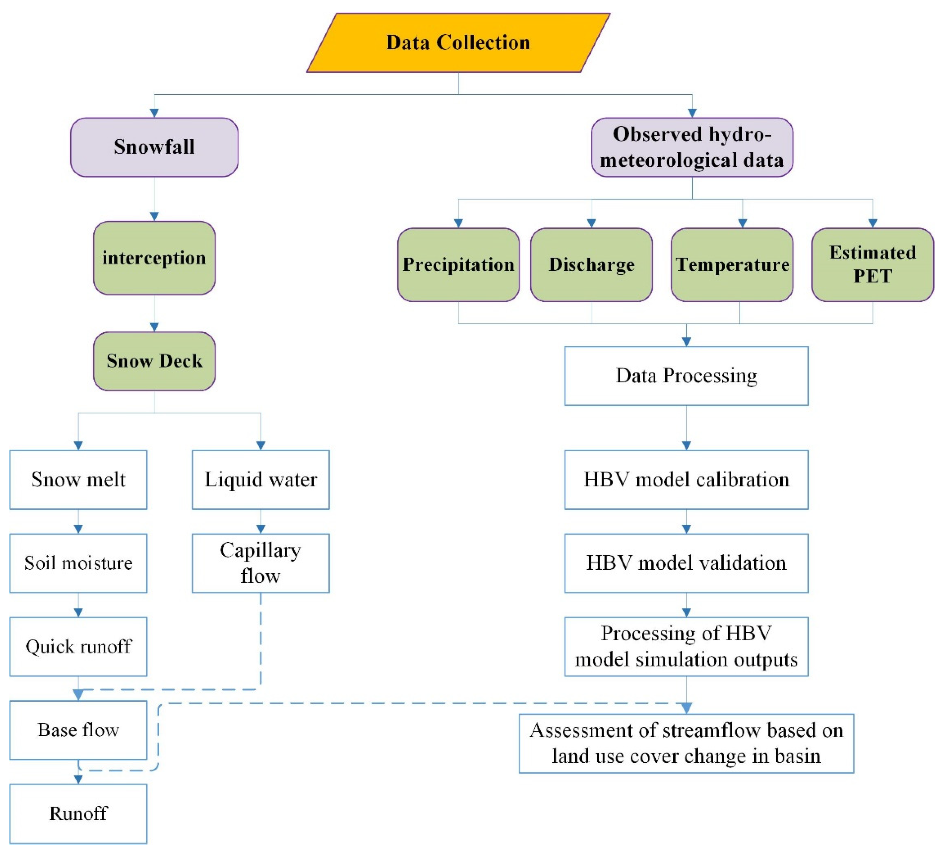
2.3. Hydrological Modeling Method

The HBV model incorporates a routine to calculate daily evapotranspiration (PETm) from monthly values. As inputs, the routine needs the long-term monthly mean potential evapotranspiration (PETm) obtained from the Thorn Thwaite method, which estimates evapotranspiration. Although this method for computing potential and actual evapotranspiration is highly accepted and widely used, it is unfeasible to perform these calculations with large data sets, such as long-term monthly temperature average (Tm) and daily mean air temperature (Td). The daily evapotranspiration was calculated by transforming (adjusting) the PETm through the difference between the Td and Tm and a coefficient C. Bergström mentioned that the adjusted potential evapotranspiration is limited to positive values and is not allowed exceeding twice the monthly average [57].
                  P E T = ( 1 + C   ·   ( T d T m ) )   ·   P E T m

2.3.1. Snowmelt and Snow Accumulation Module

The snowmelt and snow cover were supposed to be dependent upon temperature in this method. The threshold temperature (TT) was perceived as a critical design parameter for the melting and accumulation of snow at the TT. First, the TT was adjusted to −5 degrees (valid hypothesis) and then modified in the range in which the parameter could be changed. Precipitation in the form of snow occurred when a precipitation situation happened under the TT temperature; therefore, rainfall was expected [58]. The precipitation was considered in the water flow whenever the level of the average temperature rose above the TT. However, when the threshold was higher, both snow and rainfall started to contribute to the drain significantly. The snowmelt strength was measured as the amount of water from Equation (2):
S m = D D × ( T 1 T T )
where Sm is the snowmelt rate in mm/day, DD is in mm/°C/day, and T1 is the average daily temperature in °C. As described, the DD shows that the rainwater due to snow increased due to a decrease of 3 °C below the snow limit.

2.3.2. Concept of the Ice Module

A systematic daily analysis technique was used to estimate the melting of the ice, which was ultimately related to the glacier’s water absorption, and the daily ratio of snow to glacier ice was computed. The percentage of melted ice in the basin changed spatially and temporally, meaning that the meltwater outflow processes were continuously changed [59], as shown by Equation (3):
Q g = ( K G m i n + d K G × e   ( A G × S W E ) ) × S
where Q g is the snow runoff, KGmin is the minimum per day, dKG is the runoff coefficient of the glacier, and AG is a 1-mm measurement parameter. SWE is a measure of the snowpack’s water, while S is the snowpack’s water content.

2.3.3. Efficient Subcritical Rainfall

The rainfall and accumulation of snow that fell into the water runoff basin were usually divided into two sections: the original surface infiltration that participated and then the donation of external discharge. Depending on the amount of soil humidity during the rainy seasons, a surface module was computed with the HBV model. The coefficient of water content (FC) is defined as the minimum soil moisture storage in the subsurface region. A lower soil moisture content with liquid or solid precipitation indicated an increased the amount of rainfall in the flow. When the amount of water flow approached the value of the FC, the permeability decreased and the rainfall’s impact on the flow increased [60]. The precipitation was calculated with the absorption of the actual content of the water flow, as shown in Equation (4):
                                                                                    D e f f = ( S M F C ) β   ( M + S m )
where Deff is the effective precipitation in mm, SM is the net soil vapor in mm, FC is the reduction in the amount of groundwater storage in mm, M is the evaluation of daily rainfall in mm, and β is a variable. β indicates the amount of liquid (M + Sm) water that contributes to runoff. In addition, the coefficient of the runoff increases exponentially when the SM exceeds the FC.

2.3.4. Evapotranspiration Module

As an input for measuring the real evapotranspiration, the long-term mean of the monthly evapotranspiration (EPa; m = 1–12) was used. Afterwards, the reformative potential evapotranspiration was determined with respect to the time interval of the specific transmission period by using the observation that the mean daily temperature varied substantially from the actual monthly average temperature, as shown in Equation (5).
E P a = ( 1 + Z ( T T a ) ) × E P a
If EPa is adjusted as the potential evapotranspiration in mm, then T is the daily temperature standard in °C, Ta is the monthly mean in degrees, and Z is a variable. If EPa is adjusted, the soil vapor and real outcomes of the evapotranspiration are linked through the PWP (Equation (6)), which shows a relationship between water and the actual evapotranspiration.
E a c t + E P a   ( S M P W P )             If   S M   is   less   than   P W P
E a c t = E P a               If   S M   is   equal   to   P W P
Here, Eact is the maximum evapotranspiration in mm. Equation (5) clearly shows that once the moisture of the soil is equal to the PWP, the Eact actually changes at a rate opposite to that of the EPa. The PWP describes the evapotranspiration level of a soil vapor, i.e., when the SM is under the PWP, the Eact is beyond the EPa. The amount of evapotranspiration gradually decreases during soil vapor deposition [61], which is a major flaw of the PWP in Equation (6).

2.3.5. Application of Runoff

In this application, the runoff at a watershed outlet is calculated based on water storage. Water storage was used to simulate the flow of water in a near-surface system. The water storage was used to simulate a quick and steady subsurface system from a material point of view. Transport through the basins occurred at a specific constant speed of capillary action of Qperp. Once the permeable measurement in the upper part of the basin was higher than its LT sensitivity (mm], the overspill quickly followed from the upper Q0. The runoff responses of multiple outlets were smoother. The elements of monitoring (K0, K1, K2) responded to centralized storage operations. The original value of K0 was considered to be less than that of K1 to produce quick runoff. The third outlet of (Q2) response was faster than that of the second outlet (Q1), and K2 had a lower value than that of K1, as described in Equation (7):
Q0 = K0 (RuLT) If Ru is greater than LT
Q0 = 0 If Ru equals LT
Q1 = K1 × Ru
Qperc = Kperc × Ru
where Q0 is the near-surface flow in mm/day, Q1 is the interflow in mm/day, Q2 is the baseflow in mm/day, Qperp is the percolation in mm/day, K0 is the field-adjacent influx data factor, K1 is the interflow-reservoir controller for each day, K2 is the per-day baseflow storage coefficient, Kperc is a percolation storage coefficient for each day, Ru is the principal fluid storage, Ru is the secondary storage, Ru is the secondary fluid storage rank in mm, and A is a combination of the primary and secondary sources QA = (Q0 + Ql + Q2), which was achieved for the total simulated runoff QA.
Finally, for a single-input reservoir, the time-dependent model is determined as a watershed where the specific runoff Q(t) is proportional to the water saved S(t). Thus, we can obtain a (t) variable based on the coefficient of maximum storage according to Darcy’s Law (Equation (10)).
Q(t) = K × S (t)
Snow cover and water flow, as well as freezing processes, were simulated in the HBV prerendering. In addition, four-dimensional classification in the South, North, West, and East horizontal aspect categories was also improved in order to offer various effects on the snow and ice streams (Table 4). The flow of ice was transmitted by the regular historical-grade-day rain and snow routines; furthermore, the opposite behavior of the snow was attributed to the reduced surface temperature and the acceleration of the degree-day measurement to remove water [62]. The overall vegetation cover for the three cover areas showed an area of 5682 km2 at an elevation of about 5320 m.a.s.l.; the highest entire area of 424 km2 was at approximately 3600 m.a.s.l., and there was prevalent glaciation over approximately 1700 km2 between 6300 and 5200 m.a.s.l. (Table 4). The genetic algorithm and Powell (GAP) method was applied to the optimal calibrated values of the HBV parameters in forest land, pasture land, and glacier land, as presented in (Table 4).

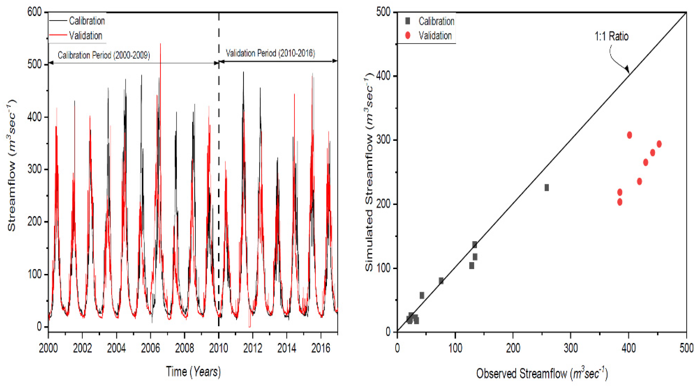
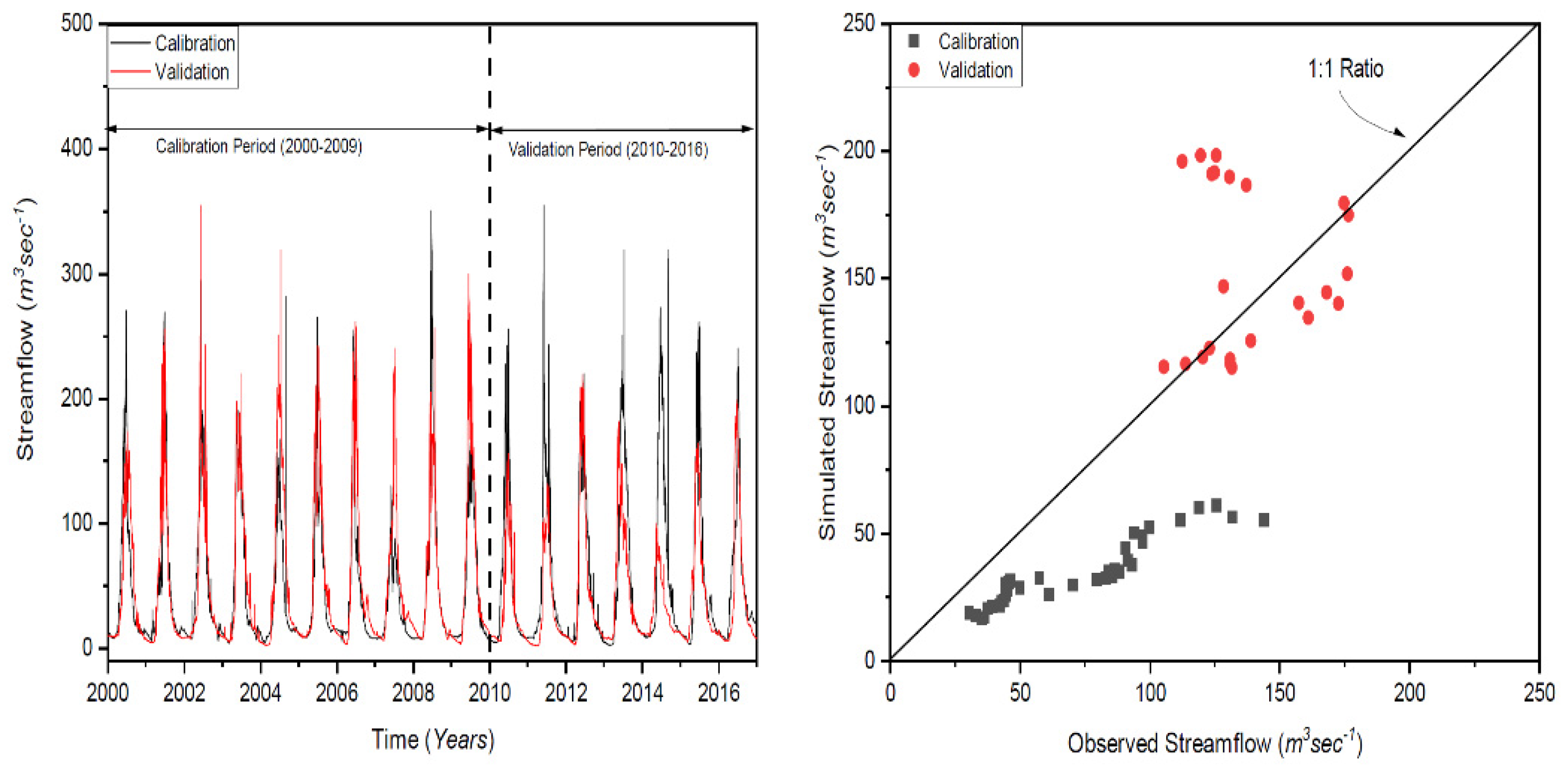
2.4. Calibration and Validation of the HBV Model in the Kunhar River Basin

The genetic algorithm and Powell (GAP) optimization approach was used for model calibration. The GAP is a stochastic design method and works evolutionarily by selecting and recombining high-performing parameter sets with each other. The GAP algorithm consists of two steps [58,59]. First, optimized parameter sets are generated by an evolutionary mechanism of selection and recombination of a set of initial, randomly selected parameter sets (again within user-defined parameter boundaries). During the second step, parameter sets are fine-tuned using Powell’s quadratically convergent method, as described in [60]. The HBV model, as for the calibration method, was used to calibrate the HBV model by the GAP method. With the GAP evolutionary method, the procedure was repeated 100 times to run the model and 1000 times additionally with Powell local optimization [61]. When running the GAP procedure 100 times, 100 different parameter data sets are computed, and then the appropriate set regarding the selected goodness-of-fit criteria is computed. Moreover, the GAP procedure was repeated to run 100 times, but with only 16 parameters (GAP16). In this way, it was tested whether the parameter values were closer to the initial ones rather than by using all 16 parameters (GAP16). A similar fixing of some of the parameters to avoid over-parameterization was done as described in [62]. The model was first calibrated for each of these time periods and then tested using validation periods selected to reflect specific climate conditions (dry, wet, warm, and cold). Each calibration period was validated by three different types of PE input data: precipitation, air temperature, and potential evapotranspiration. The analysis encompassed the entire study period, and the validation periods did not overlap. The procedure is schematically presented in Figure 1. The hydrological model with input data and with known model parameters shown in Table 1 was calculated. The HBV model’s performance with the set of parameters was calibrated (2000–2009) and validated (2010–2016) for Gari-Habibullah and Naran, which accurately represent the Kunhar River Basin’s hydrological characteristics (Table 5). The principal origin of the river that flows into the Kunhar watershed is ice, glacier runoff, and rainfall. For this reason, the criteria of the parameters were selected based on these river flow origins. The HBV model frequently ran throughout the calibration and validation for Gari-Habibullah and Naran and worked consistently well between the calibration and validation stages, with Nash–Sutcliffe (NSE) efficiency values of 0.87 and 0.79 around the basin. The relationship between the simulated and observed river flows in the calibration and validation periods became extremely good, with NSE values of 0.87 and 0.79, respectively (Figure 4 and Figure 5). The model reflected excess discharge in 2006 in Gari-Habibullah and high discharge in 2007 during the calibration process, whereas in 2011 and 2015, the discharge was unpredictable and significantly overstated throughout the validation period.
The year 2013 was reported as one of Pakistan’s warmest times. The highest average temperature in northern Pakistan was 47.5 °C on 19 July 2013. The temperature might have increased stream flows through excessive ice melting and melting of glaciers, but this was not effectively identified by the model due to undervaluation of the river flows in 2013. By comparison, the years 2011 and 2015 were also mentioned in Pakistan’s unpredictable weather history, which is the justification for the accurate assessments; these may be irregularities in the existing meteorological data. Likewise, for the validation period, in Pakistan, 2013 was one of the warmest years, and the temperatures in different regions of the country ranged from 47 to 51 °C. Briefly, the causes behind our overestimations of the projected stream flows may be due to mistakes made with the climate index method in the simulation system, inadequate seasonal rainfall, or extreme precipitation in certain seasons. Similarly, in a past analysis, the seasonal river flows throughout the Kunhar River Basin were uncertain [8]. The hypothesized inadequate seasonal flow in the Kunhar River Basin was focused on environmental impacts relative to several other inadequate catchments in the Upper Indus Basin (UIB), Pakistan, which are dependent on winter rainfall and early spring flow in the Kunhar River Basin. Furthermore, various conditions influence the melting of ice and glaciers, including the landscape, weather, dimensions, elevation, hillsides, and soil types of the region, whether intentionally or unintentionally. After all, the weather scale approach does not accurately describe certain parameters [63]. PBIAS revealed unfavorable results of 0.47 and 14.61, indicating that the calibration and validation cycles were inadequate for the actual model (Table 5). The maximum projected discharge was 582 mm per year for the calibration period (2000–2009) and 592 mm for the measured flow, indicating a clear correlation between the projected and measured flow. For the 2010–2016 validation periods, the average yearly discharge from the simulation and analysis was 488 and 495 mm, respectively. For both the calibration and validation periods, the average error (AE), average absolute error (AAE), and standard error (SE) were minimal (Figure 4 and Figure 5). The relationship between the actual and the measured streamflow was strong, with determination coefficients (R2) of 0.95 and 0.94 simultaneously across the periods of calibration and validation. The model significantly estimated the river discharge on a regular basis in 2004, but underestimated it significantly during the calibration period in 2004 and 2006. During the validation, the same river flow as on the regular basis underestimated the river discharge in 2011 and 2012 and overstated it significantly in 2013. During both calibration and validation, the model underestimated the seasonal streams.
To evaluate the efficiency coefficient, a statistical approach was performed to determine the hydrological system’s predictive control with the Nash–Sutcliffe (NSE) efficiency coefficient [51]. It is defined as
R e f f = 1 Σ ( Q o b s Q s i m ) 2 Σ ( Q o b s Q o b s ) 2
where Qobs is observed, Qsim is simulated, and R e f f is the NSE. A reference value of 1 shows an absolutely ideal match. Calibration and validation, which resulted in NSE values of 0.87 and 0.79 around the basin, were highly effective in the HBV model (Figure 3). After achieving these parameters for the HBV model, the expected river flow changes for the periods of 2017–2037 (near), 2038–2058 (mid), and 2059–2079 (far) were incorporated into the HBV. This was based on four GCMs and four RCP scenarios.

2.5. Comparison in Each Time Scale (Daily/Monthly/Seasonal)

At the daily scale, the statistical results show no significant difference between the GCMs rain data, with CC of 0.39/0.48 and AAE values of 14.3/16.4, respectively (Table 6). A difference is found in that the GCMs’ values underestimated the actual precipitation, with a PBIAS value of −15.24%, while RCPs overestimated the actual precipitation with a PBIAS of 98.4%. Therefore, the AE value of the GCMs is also much higher than that of the RCPs, with values of 7.3 and 5.8 mm/day, respectively.
As predicted, the trend described above is also seen on the monthly scale. The CC values of the RCP data ranged from 0.39 to 0.48, showing a good correlation with the GCMs’ data. Moreover, the AE and AAE values of the GCMs are many times higher than those of the RCPs. The errors at the daily scale were eliminated by the aggregation to the monthly scale, causing the CC to become more balanced; however, this does not explain the big difference observed in the evaluation trends between GCMs. The GCMs’ precipitation data is always overestimated across the basin, and the largest bias statistic indicator values were recognized with this dataset in evaluations by Mou Tan et al. (2017) [64] and Roth Lemann et al. (2016) [65]. Generally, the GCMs’ precipitation data are slightly more accurate and agree relatively better than the RCPs’ data with observations measured on the monthly scale. As shown in Table 6, the analysis results of the seasonal statistical indicators obtained from the RCPs’ data show the largest mean errors, with AE and AAE values that are too large. At the same time, the PBIAS value of the GCMs in the dry season is −39.8%, many times different from the rainy season value of −7.3%. This is related to the very low GCMs’ rainfall that occurs in the dry season; the lower rainfall value in the denominator of Equation (7) will cause the PBIAS value to be higher. Due to underestimating rainfall in the dry season, the rainfall in the GCMs’ data makes the difference between the two seasons much larger than the observed data. The rainfall ratios between the dry and rainy seasons for GCMs were 17% and 93%, respectively.

3. Results

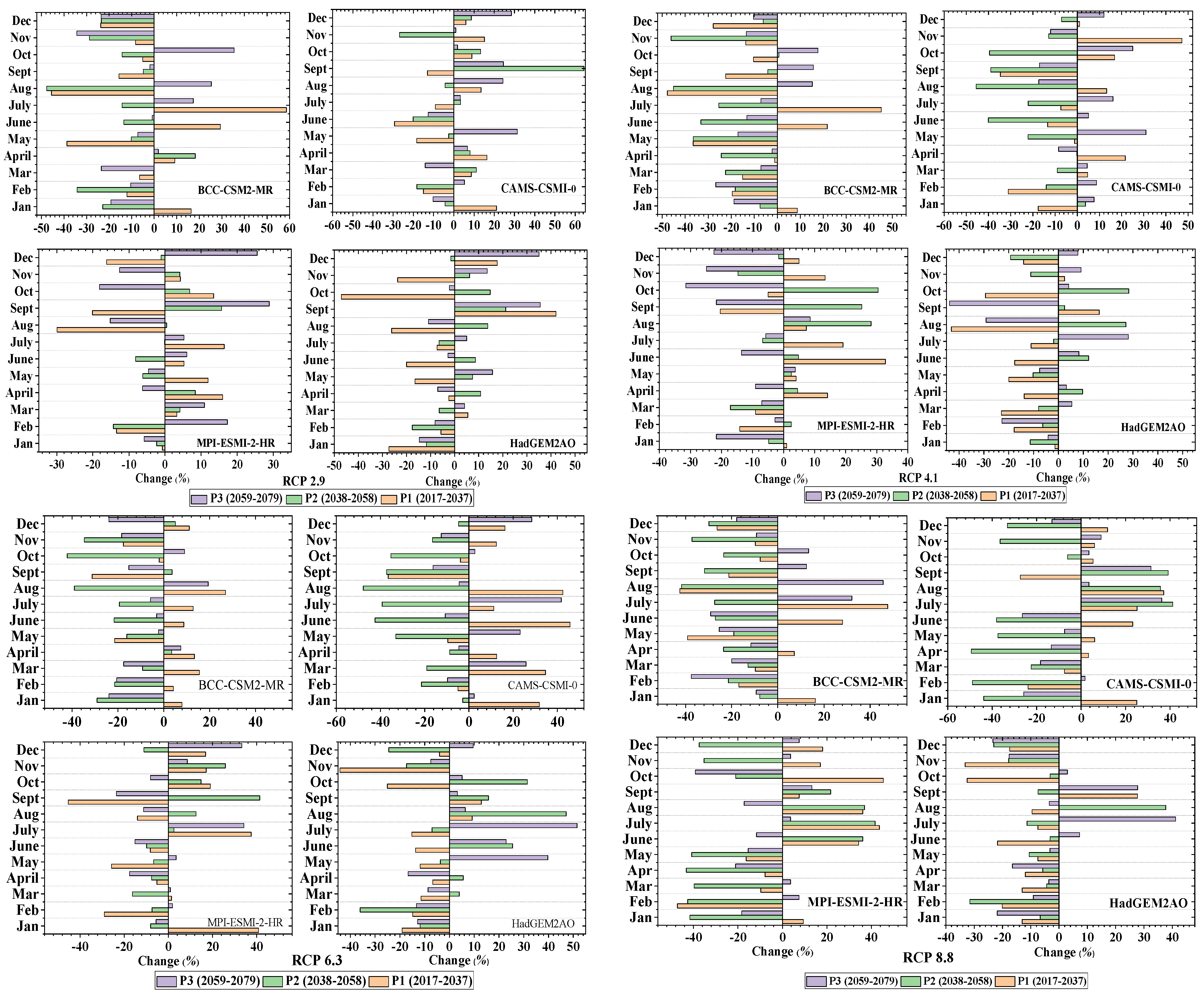
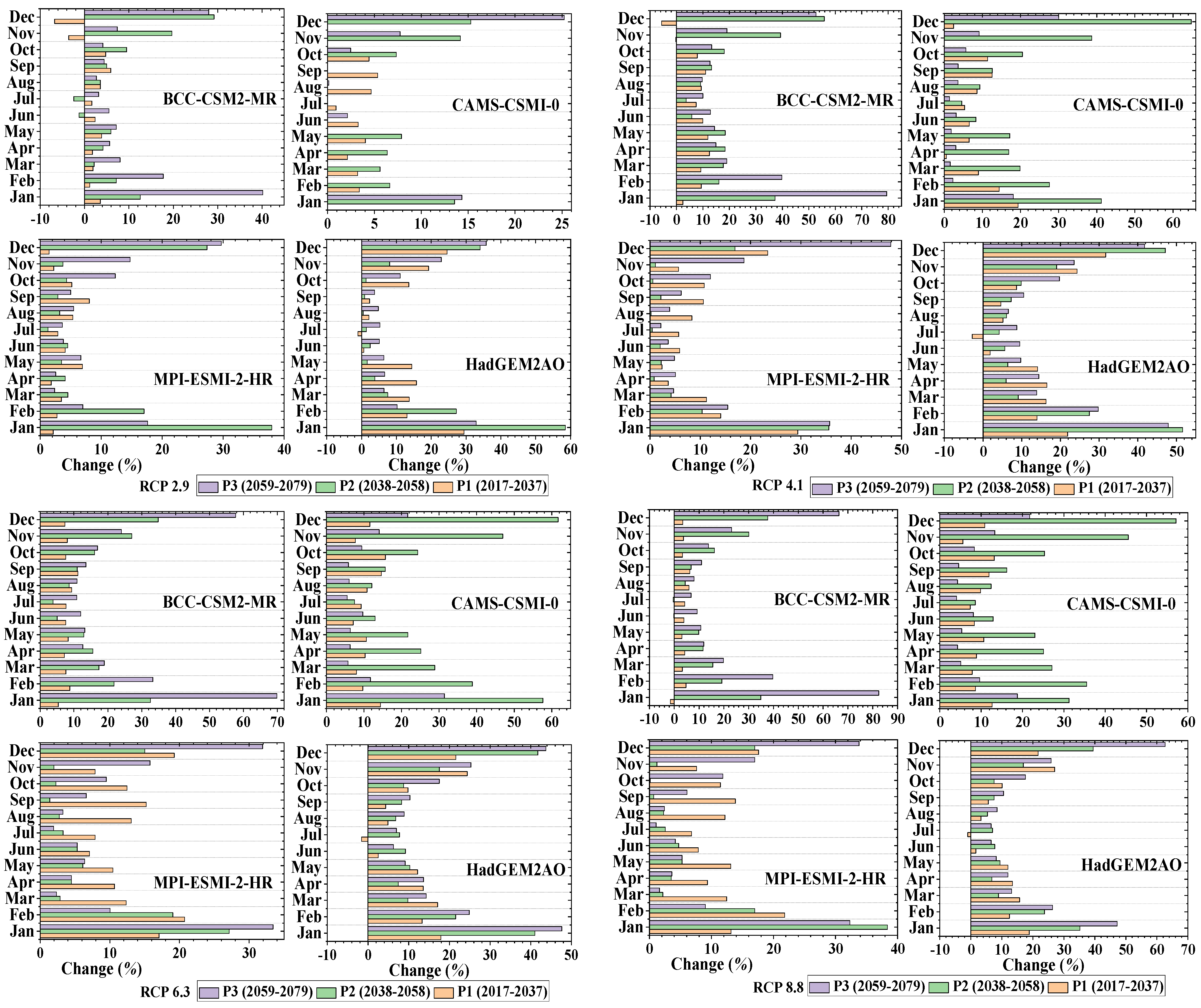
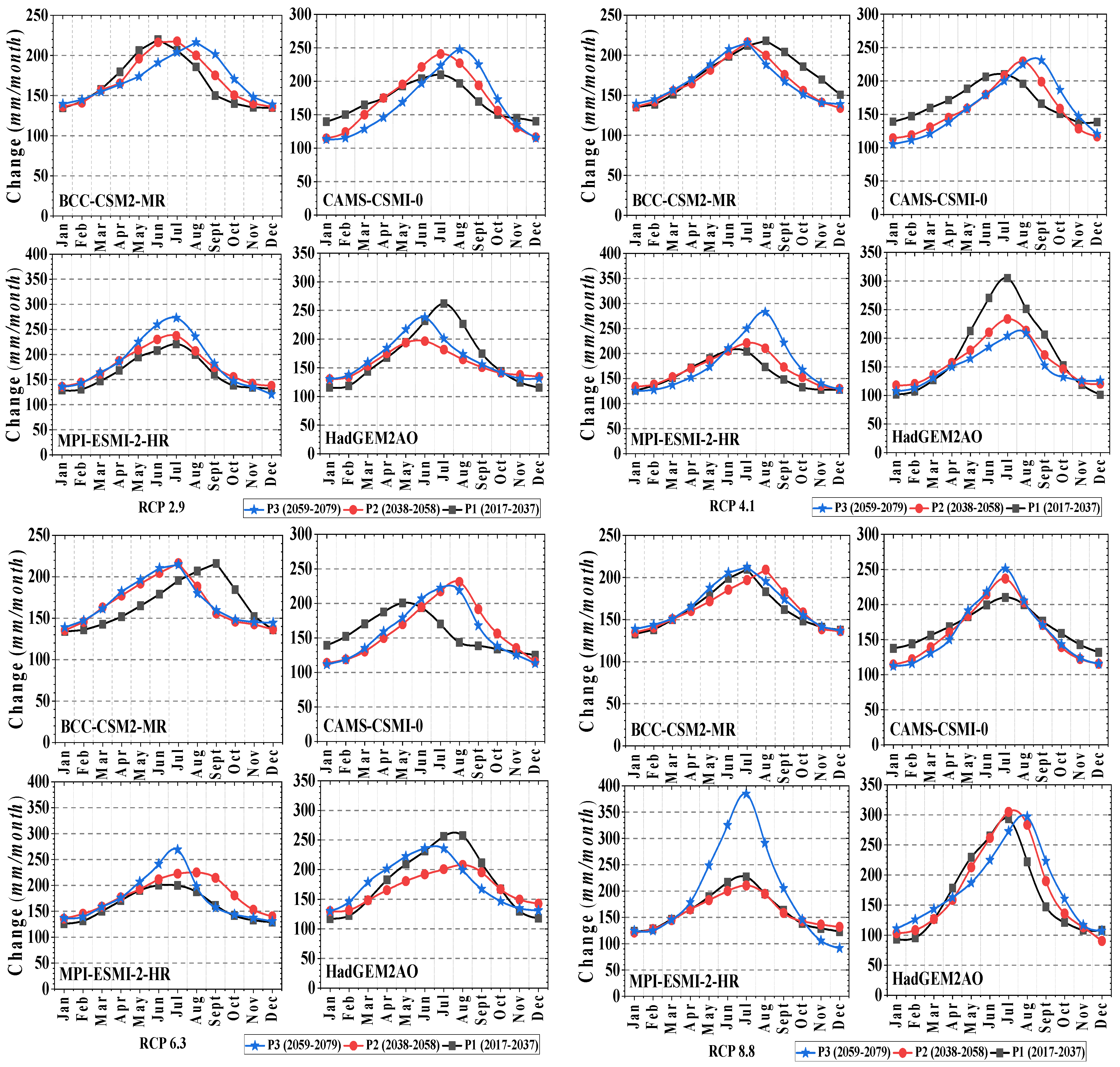
3.1. Projected Changes in Precipitation

Expected increases in the monthly precipitation in GCMs of the near, mid, and far future for the four RCPs were estimated through a model simulation (Figure 6). In the warm weather and in early fall, precipitation significantly increases when using CAMS-CSM1-0, showing an increase of up to 58% for return intervals in a deep-term period and 38% percent for the progressing monsoon months in the mid-future period in the RCP 2.9 emission scenario. In the RCP 4.1 emission scenario, BCC-CSM2-MR has an increase of 60% in early monsoon precipitation in the approximated future, although CAMS-CSM1-0 indicates a reduction of approximately 48% in the autumn period in the long term. HadGEM2AO has a forecast for a 61% rise in the beginning of the monsoon cycle for the near future, while CAMS-CSM1-0 predicts a 47% decrease in the advancing monsoon season duration for the upcoming future timeframe in the RCP 6.3 emission scenario. BCC-CSM2-MR estimates an incredible 139% shift in the start date of the monsoon. For the relatively near-future period, a significant 93% decrease is assumed according to the MPI-ESMI-2-HR project in the RCP 8.8 emission scenario. The general opinion in the identification of relevant plans is that there will be an indicative liquid precipitation increase (from the rainy season) and an increase in the intensity of rainfall (from the cold season) in the future, according to the results from the watershed [66].

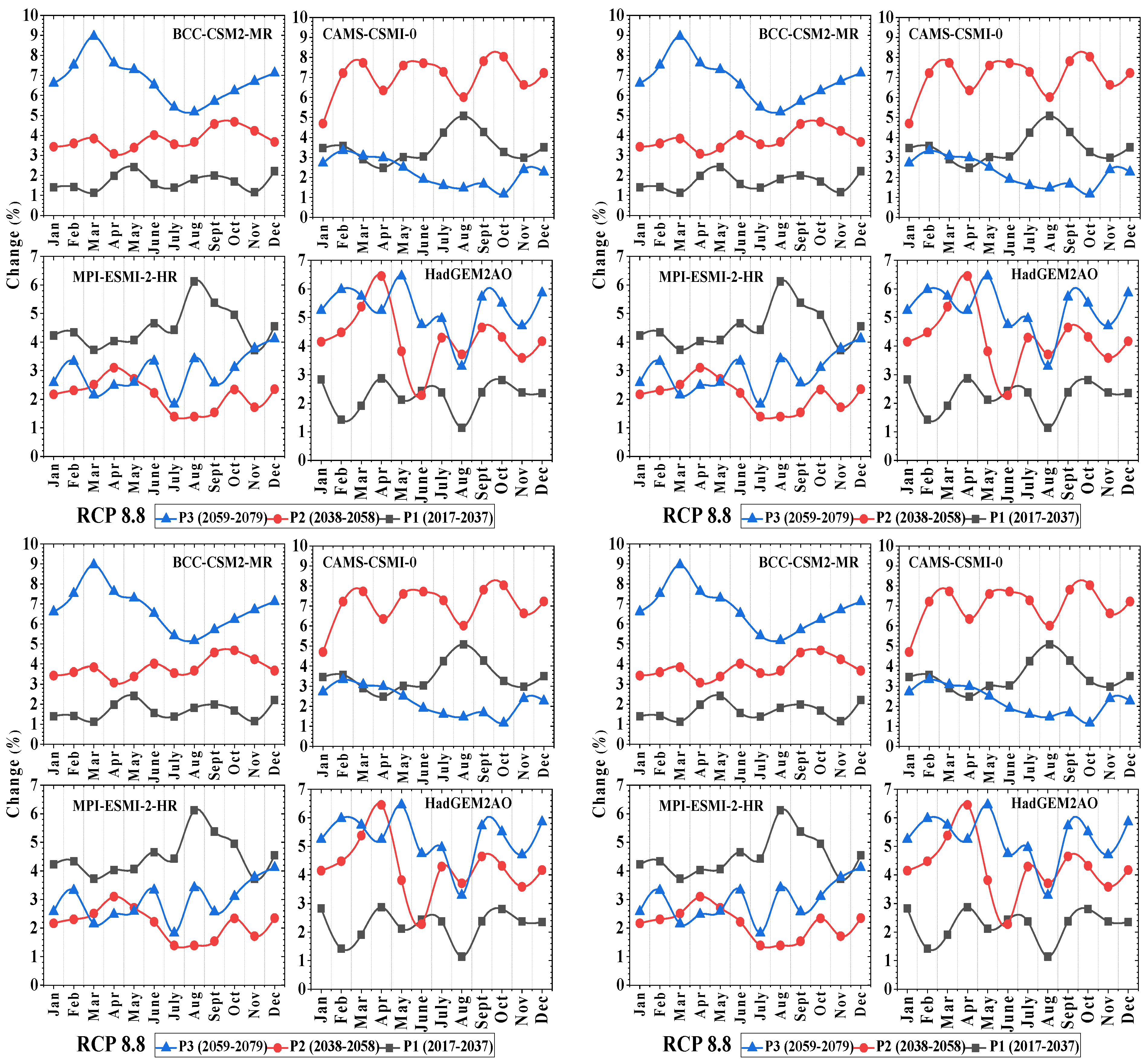
3.2. Projected Changes in Temperature

The predicted periodic temperature changes for four RCPs of the GCMs are shown in Figure 7. The temperatures of the Kunhar River Basin are predicted to rise, on average, until around the end of the decade. According to MPI-ESMI-2-HR, an increase of up to 3.5 °C was recorded in the RCP 2.9 emission scenario during summer-to-winter transition months in the future. According to the MPI-ESMI-2-HR data, a much greater increase of 4.5 °C is expected during the winter-to-summer transition months. In addition, cold-to-warm transition seasons are predicted with MPI-ESMI-2-HR in the RCP 6.3 emission scenario to rise 5.6 °C higher than RCPs 2.9 and 4.1 throughout the winter. Moreover, during the cold-to-warm transition period, an alarming 8.5 °C increase (the maximum increase among all RCPs), as indicated by MPI-ESMI-2-HR, would occur in the future under the RCP 8.8 scenario. All of the simulations of the temperature assume that the period for which the snow stays is likely to reduce the glacial period’s metamorphic phase due to the massive variations in all of the emission scenarios across the watershed. In other words, due to the start of mid-summer that is predicted for the basin, a significant glacial reduction is expected [67].

3.3. Projected Changes in Evapotranspiration

The increases in quarterly evapotranspiration expected were described for four RCPs of the GCMs (Figure 8). For the mid- and long-term winter peaks, the highest enhancement of 46% was reported under the MPI-ESMI-2-HR emission scenario with RCP 2.9. In the highest recorded winter months, a greater increase of up to 64% can be seen for the far-future timeframe, as defined by the MPI-ESMI-2-HR in the RCP 4.1 emission scenario. Furthermore, a significant increase of up to 69% was observed in the coldest months for future periods predicted in the RCP 6.3 emission scenario for MPI-ESMI-2-HR. Furthermore, an impressive 98% change was recorded for the coldest months in the extended period, as shown by MPI-ESMI-2-HR in the RCP 8.8 emission scenario.

3.4. Projected Changes in Stream Flow

The maximum flow variability in the RCP 8.8 emission scenario was calculated (Figure 9). With BCC-CSM2-MR, monsoon flow is expected to rise by up to 42% in the mid future, while for MPI-ESMI-2-HR, it is projected to decrease by up to 19% in the winter months in the long-term RCP 2.9 emission scenario. The monsoon flow in the next few months showed a rise of up to 63%, and in the extreme winter months, it showed an increase of up to 34% in the middle of the next half according to the IPSL-CM5A-LR state in the RCP 4.1 emission scenario. CAMS-CSM1-0 forecasted a rise of up to 76% in progressive rainy season stream flow over several months, while the RCP 6.3 emission scenario projected a decrease of up to 21% in the peak cold months in the long term. In addition, CAMS-CSM1-0 projected an increase of up to 149% during monsoon initiation periods for the far-future period, and with MPI-ESMI-2-HR, the fall flows are expected to drop to 36% in the RCP 8.8 emission scenario. It was observed that all GCM results are compatible in the direction of flow changes in each emission scenario. Simultaneously, a series of small variations were reported for the river streams during the forecast periods. The effects of the water flow measurements indicate a significant increase in hot season water flows and a complete decline in cold season water flows. This could be due to the essential rise in spring temperatures, which contributed to the monsoon months and significant winter evapotranspiration changes in the GCMs. After all, the measurements of the rapidly increasing flows substantially exceed the amounts of decreasing flows in all estimates that were compatible with the results [68].

4. Discussion

In the mountain region of the Kunhar River basin Pakistan, the large amount of precipitation leads to a substantial accumulation of snow during the winter and spring season. The stream flow increases rapidly with the beginning of the snow melting period in March and April. The Kunhar River Basin receives its maximum precipitation in winter and spring, which results in a clear temporal separation in accumulation of the snow and the time of the peak flow. The Kunhar River is characterized by a seasonal cycle of river flow with maximum flow in the summer season. Summer runoff of the upstream catchments of the Southern Asian Rivers is controlled by the melting of snow and glaciers, which, in glacierized catchments, contributes up to 50% of the seasonal flow [69]. The downscaled precipitation and maximum/minimum temperature estimates from the five GCMs were in good agreement with the measurement-based data under the baseline condition. The product of multiple GCMs of the Intersectoral Impact Model Intercomparison Project (ISI-MIP) was used to assess the influences of the climate variation on the hydrological regimes, considered a suitable representative [48,70,71].
The meteorological data from four climate stations and streamflow data from one hydrological station were used in this study. We analyzed the possible consequence of projected climate variation on interseasonal and annual water flow, as well as on snowmelt in the Kunhar River basin. We studied the responses of hydrological processes, such as discharge and extreme and median flows, to climate variation. The temporal impacts of the projected climate change were assessed by coupling a well-calibrated semidistributed hydrological model (HBV) with the results of the five GCMs under two greenhouse gas emission scenarios (RCP 4.1 and RCP 8.8). The effect of topography was corrected by applying the elevation band (temperature lapse rate and precipitation lapse rate) approach in this study, which improved the simulation results. We presented the results of the streamflow calibration and validation for the Kunhar River. Additionally, by using the HBV tool, we studied the sensitivity and prediction uncertainty of the model parameters, which was necessary to evaluate the strength of the calibrated model. The results of the GCMs presented continuous warming over the Kunhar River basin at the annual and seasonal scales in the middle and at the end of this century.
This finding is consistent with the results of previous studies in the South and Central Asian regions, including the Pamir-Alay [72,73], the Tian Shan–Pamir–North Karakoram [74], the Himalayas [75], and the Tibetan Plateau [76]. It is expected that the wet and dry seasons in the basin will become more severe than those in the baseline period. We showed that these phenomena are predicted to be stronger under RCP 8.8 than under RCP 4.1. A possible reason for these alterations is that in the future, more meltwater will be produced in early summer and more snow will be replaced by rain. The typical changes will accelerate the convergence of water flows and raise the flooding frequency and intensity. Folini et al. [77] reported that aerosol emissions in the 20th century might increase, in association with the enormous population and industrialization growth. Similarly, Bollasina et al. [78] confirmed that in Asia, the concentration of atmospheric aerosols has increased steadily.
Xin et al. [79] reported that over China and Central Asia, a rising trend in the concentration of aerosols in the atmosphere could cause a substantial rise in temperature. The mean annual precipitation over the Kunhar River basin is expected to rise in the 2038–2058 future time period under RCP 4.1, as evidenced by the results of two GCMs (CAMS-CSM1-0 and HadGEM2AO), as well as the two GCMs (MPI-ESMI-2-HR and HaDGEM2AO) that indicated a rising trend of precipitation in the second time period (2059–2079) under RCP 8.8. The remaining GCM models that were analyzed in this study showed a decreasing trend of mean annual precipitation in the two future periods under both RCPs. The winter mean precipitation had a lower decreasing trend than that of the summer and fall seasons. The summer mean precipitation exhibited a greater decreasing tendency than the other seasons in the two future periods. Similarly, in the Yellow and Xin River Basins in China [80], in the Middle East [71], and in the westerly dominated region of South Asia, a decreasing trend of summer precipitation was indicated [81]. The increasing or decreasing propensity of winter precipitation varies from model to model. Two GCMs showing a rising trend of winter precipitation and resembling this analysis were reported by Luo et al. [82] for the Heihe River Basin and by Omani et al. [83] for the Pamir-Alay Mountains in Central Asia. However, the patterns of seasonal variations in precipitation for three GCMs presented in the Kunhar River Basin are contrary to those in reported for the Hunza River Basin of the Karakoram Mountains [84] and the Jhelum River Basin of the Himalayan Mountains [74]. Pendergrass et al. [85] reported that the global winter precipitation increased over the second half of the 20th century, and they attributed this to the role of increasing moisture counteracted by weakening circulation. Li et al. [86] pointed out that in Central Asia, at the end of 20th century, there was a persistent decreasing trend of annual precipitation, and Meng et al. [87] confirmed that precipitation might increase in the middle of the 21st century in the south of the Tian Shan Mountains. The multimodel ensemble result projected a decrease in average annual precipitation during the 2038–2058 and 2059–2079 time periods under both RCPs in the Kunhar River basin. The interannual and seasonal scale analyses of the mean precipitation changes presented large uncertainties among the GCMs, as evidenced by both increasing and decreasing tendencies under RCP 4.1 and RCP 8.8 in various future time periods. In the Asian region, these contradictions in our findings may be associated with the rising concentration of anthropogenic absorbing aerosols and the westerlies system [73,74]. The analysis of the simulated Kunhar River flows mostly described an increasing trend of the mean annual streamflow during the 2059–2079 time period under RCP 4.1 and RCP 8.8, as well as a decreasing trend during the 2038–2058 time period under RCP 4.1. Mostly, the increase and a lesser decrease of annual future flow may be attributed to the similar projection of the different GCM models for the total annual precipitation. Similarly, a decreasing/increasing tendency for the different future periods of annual river flow was indicated in an arid alpine catchment in Karakoram [81]. In addition, it is expected that the average monthly peak discharge may shift to earlier in the summer season, from July to June, for the two future time periods under both RCP 4.1 and RCP 8.8 for almost all GCMs, which is mainly due to the slight rise in precipitation in the spring and winter seasons, as well as because of an earlier snowmelt caused by global warming. Similarly, due to earlier snowmelt, Sorg et al. [88] projected the impacts of climate changes on flow seasonality and concluded that less water will be available in the summer months in the Syr Darya River Basin in Central Asia. Olsson et al. [89] confirmed, from trend analysis, this shift in seasonality of flow and predicted a possible decreasing trend of annual flow in the Zarafshan River Basin in Central Asia. A similar shift in the discharge peak (July to June) was pointed out by Liu et al. [90] for the Yarkant River Basin in Central Asia; in contrast, Babur et al. [91] reported that the discharge peak could be delayed (July to August) in the Jhelum River Basin. These discrepancies in detections might be related to various projected climate models for winter and summer seasonal precipitation in Central Asia. We found that the average monthly peak discharge in the Kunhar River Basin indicated a significant decreasing tendency in August and September for the 2038–2058 and 2059–2079 time periods under RCP 4.1 and RCP 8.8 for all five of the GCMs. In this study, most of the GCM model outputs along with the multimodel ensemble results showed that the summer water flow in the Kunhar River is expected to increase at the end of the 21st century under the two studied greenhouse gas emissions scenarios. Increases in summer water flow in the Kunhar River can be ascribed to the rapidly melting snow and ice caused by the continuously increasing air temperature. Meanwhile, it could lead to uncertainty in the predictions due to fluctuations in the reduction of sea ice and the gradual increase in the snow lining. Furthermore, these conditions are predictable if the temperature in all GCMs increases significantly.

5. Conclusions

This study is the first to refer to the role of temperature in extreme events based on regulations in the Kunhar River Basin. The temperature verification in the Kunhar River Basin shows that RCP scenarios can be representative as ground temperature measurement stations in meteorological and hydrological studies. Temperature events, such as very cold, damaging cold, strong sun, and scorching hot events, affect the rainfall distribution and the inputs to the flow simulations. Moreover, the proposed study is suitable for humid climate conditions in the tropics, such as the climatic conditions in the study area, and can be reliably used in other basins with similar conditions. After incorporating all of the appropriate hydrometeorological data, an HBV model was developed on a daily time scale. First, the model was calibrated and validated using parameters from 2000 to 2016. The predicted flow variation in the Kunhar River Basin was calculated using statistically decreased high-resolution GCM performance as an input for hydrological HBV models under different RCP emission scenarios. The level of maximum rainfall was almost 1650 mm in the wind-retrieval and fall months, with a maximum temperature of 23 °C during the starting months of the rainy season.
The maximum evapotranspiration was almost 4 mm during the starting months of the rainy season, and the highest discharge of flow was about 1032 m3/s along the basin; these values show the yearly climatology of the hydrometeorological parameters. The HBV model for stream flow projection included a snow melting and snow accumulation module, ice module, efficient subcritical rainfall, evapotranspiration module, and an application of runoff. This highly effective HBV model was used for calibration and validation, with NSE values of 0.87 and 0.79, respectively. Postprocessing is expected to significantly improve the predictions of liquid precipitation and consistency (winter) in future precipitation slices. The temperature predictions of all of the simulations suggest that the snow residence period is likely to decrease for the metamorphic cycle of glaciation due to significant improvements in all of the basin’s emission scenarios. The results also show that the summer streamflow over the basin is expected to significantly increase, as shown by the analysis of the simulations’ performance. The advantages and disadvantages of study suggest that local knowledge/information is also very useful in hydrometeorological research to avoid excessive misunderstandings of gridded climate scenarios and can instead be understood as an opportunity to explore the potential of reanalyzing data in terms of their performances that are, as of yet, unproven due to limited, short duration, and heterogeneous observational data. Our tentative studies will be further expanded with other gridded climate scenarios already recognized in Pakistan, and the spatial variations in water balance components and the effects of climate change on flow changes in the Kunhar River Basin will be calculated. This study’s findings are essential because emission-based hydrometeorological simulations of the Kunhar River Basin and the multi-GCM output differences across the river’s watershed have been insufficiently studied.

Author Contributions

Conceptualization, C.H.; Methodology, S.-e.-h.S.; Software, S.-e.-h.S. and Q.W.; Validation, C.H., S.-e.-h.S. and L.Z.; Formal analysis, S.-e.-h.S.; Investigation, S.-e.-h.S., M.W.B. and M.H.A.A.S.; Resources, C.H.; Data curation, S.-e.-h.S.; Writing—original draft preparation, S.-e.-h.S.; Writing—review and editing, C.H. All authors have read and agreed to the published version of the manuscript.

Funding

This work was funded by the Projects of National Natural Science Foundation of China (51979250), Key projects of National Natural Science Foundation of China (51739009), and Key Research and Promotion Projects (Technological development) in Henan Province (202102310587).

Data Availability Statement

Data cannot be made publicly available; readers should contact the corresponding author for details.

Acknowledgments

It is the author’s wish to acknowledge and thank the Pakistan Meteorological Department (PMD), as well as the Water Development Authority (WAPDA) of Pakistan, for providing important and valuable data for this research.

Conflicts of Interest

The authors declare no conflict of interest.

References

  1. Ludwig, F.; van Slobbe, E.; Cofino, W. Climate change adaptation and Integrated Water Resource Management in the water sector. J. Hydrol. 2014, 518, 235–242. [Google Scholar] [CrossRef]
  2. Naeem, U.A.; Hashmi, H.N.; Shakir, A.S. Flow trends in river Chitral due to different scenarios of glaciated extent. KSCE J. Civ. Eng. 2013, 17, 244–251. [Google Scholar] [CrossRef]
  3. Taylor, R.G.; Scanlon, B.; Döll, P.; Rodell, M.; van Beek, R.; Wada, Y.; Longuevergne, L.; Leblanc, M.; Famiglietti, J.S.; Edmunds, M.; et al. Ground water and climate change. Nat. Clim. Chang. 2013, 3, 322–332. [Google Scholar] [CrossRef] [Green Version]
  4. Green, T.R.; Taniguchi, M.; Kooi, H.; Gurdak, J.J.; Allen, D.M.; Hiscock, K.M.; Treidel, H.; Aureli, A. Beneath the surface of global change: Impacts of climate change on groundwater. J. Hydrol. 2011, 405, 532–560. [Google Scholar] [CrossRef] [Green Version]
  5. Goderniaux, P.; Brouyère, S.; Fowler, H.J.; Blenkinsop, S.; Therrien, R.; Orban, P.; Dassargues, A. Large scale surface-subsurface hydrological model to assess climate change impacts on groundwater reserves. J. Hydrol. 2009, 373, 122–138. [Google Scholar] [CrossRef]
  6. Eckhardt, K.; Ulbrich, U. Potential impacts of climate change on groundwater recharge and streamflow in a central European low mountain range. J. Hydrol. 2003, 284, 244–252. [Google Scholar] [CrossRef]
  7. Iqbal, M.S.; Dahri, Z.H.; Querner, E.P.; Khan, A.; Hofstra, N. Impact of climate change on flood frequency and intensity in the Kabul River Basin. Geosciences 2018, 8, 114. [Google Scholar] [CrossRef] [Green Version]
  8. Akhtar, M.; Ahmad, N.; Booij, M.J. The impact of climate change on the water resources of Hindukush–Karakorum–Himalaya region under different glacier coverage scenarios. J. Hydrol. 2008, 355, 148–163. [Google Scholar] [CrossRef]
  9. Srivastava, A.; Sahoo, B.; Raghuwanshi, N.S.; Singh, R. Evaluation of Variable-Infiltration Capacity Model and MODIS-Terra Satellite-Derived Grid-Scale Evapotranspiration Estimates in a River Basin with Tropical Monsoon-Type Climatology. J. Irrig. Drain. Eng. 2017, 143, 04017028. [Google Scholar] [CrossRef] [Green Version]
  10. Srivastava, A.; Deb, P.; Kumari, N. Multi-Model Approach to Assess the Dynamics of Hydrologic Components in a Tropical Ecosystem. Water Resour. Manag. 2020, 34, 327–341. [Google Scholar] [CrossRef]
  11. Paul, P.K.; Kumari, N.; Panigrahi, N.; Mishra, A.; Singh, R. Implementation of cell-to-cell routing scheme in a large scale conceptual hydrological model. Environ. Model. Softw. 2018, 101, 23–33. [Google Scholar] [CrossRef]
  12. Langsholt, E.; Lawrence, D.; Wong, W.; Andjelic, M.; Ivkovic, M.; Vujadinovic, M. Effects of Climate Change in the Kolubara and Toplica Catchments, Serbia; Norwegian Water Resources and Energy Directorate: Oslo, Norway, 2013. [Google Scholar]
  13. Shiwakoti, S. Hydrological modeling and climate change impact assessment using HBV light model: A case study of Karnali River basin. Iran. J. Energy Environ. 2017, 8, 296–304. [Google Scholar]
  14. Hock, R. Glacier melt: A review of processes and their modelling. Prog. Phys. Geogr. 2005, 29, 362–391. [Google Scholar] [CrossRef]
  15. Kay, A.; Davies, H.; Bell, V.; Jones, R. Comparison of uncertainty sources for climate change impacts: Flood frequency in England. Clim. Chang. 2009, 92, 41–63. [Google Scholar] [CrossRef]
  16. Konz, M.; Seibert, J. On the value of glacier mass balances for hydrological model calibration. J. Hydrol. 2010, 385, 238–246. [Google Scholar] [CrossRef] [Green Version]
  17. Hay, L.E.; Wilby, R.L.; Leavesley, G.H. A comparison of delta change and downscaled GCM scenarios for three mountainous basins in the United States 1. J. Am. Water Resour. Assoc. 2000, 36, 387–397. [Google Scholar] [CrossRef]
  18. Wilby, R.L.; Hay, L.E.; Gutowski, W.J., Jr.; Arritt, R.W.; Takle, E.S.; Pan, Z.; Leavesley, G.H.; Clark, M.P. Hydrological responses to dynamically and statistically downscaled climate model output. Geophys. Res. Lett. 2000, 27, 1199–1202. [Google Scholar] [CrossRef] [Green Version]
  19. Chu, J.; Xia, J.; Xu, C.-Y.; Singh, V. Statistical downscaling of daily mean temperature, pan evaporation and precipitation for climate change scenarios in Haihe River, China. Theor. Appl. Climatol. 2010, 99, 149–161. [Google Scholar] [CrossRef]
  20. Thompson, J.; Green, A.; Kingston, D.; Gosling, S. Assessment of uncertainty in river flow projections for the Mekong River using multiple GCMs and hydrological models. J. Hydrol. 2013, 486, 1–30. [Google Scholar] [CrossRef]
  21. Mahmood, R.; Babel, M.S. Evaluation of SDSM developed by annual and monthly sub-models for downscaling temperature and precipitation in the Jhelum basin, Pakistan and India. Theor. Appl. Climatol. 2013, 113, 27–44. [Google Scholar] [CrossRef]
  22. Houben, G.; Tünnermeier, T.; Eqrar, N.; Himmelsbach, T. Hydrogeology of the Kabul Basin (Afghanistan), part II: Groundwater geochemistry. Hydrogeol. J. 2009, 17, 935–948. [Google Scholar] [CrossRef]
  23. Sarwar, S. Reservoir Life Expectancy in Relation to Climate and Land-Use Changes: Case Study of the Mangla Reservoir in Pakistan. Ph.D. Thesis, University of Waikato, Hamilton, New Zealand, 2013. [Google Scholar]
  24. Ali, S.; Li, D.; Congbin, F.; Khan, F. Twenty first century climatic and hydrological changes over Upper Indus Basin of Himalayan region of Pakistan. Environ. Res. Lett. 2015, 10, 014007. [Google Scholar] [CrossRef]
  25. Hewitt, K.; Young, G. Snow and ice hydrology project: Upper Indus basin. Overall Rep. Can. Cent. 1990, 4, 203–232. [Google Scholar]
  26. Irmak, S.; Irmak, A.; Allen, R.; Jones, J. Solar and net radiation-based equations to estimate reference evapotranspiration in humid climates. J. Irrig. Drain. Eng. 2003, 129, 336–347. [Google Scholar] [CrossRef]
  27. Bocchiola, D.; Diolaiuti, G.; Soncini, A.; Mihalcea, C.; D’agata, C.; Mayer, C.; Lambrecht, A.; Rosso, R.; Smiraglia, C. Prediction of future hydrological regimes in poorly gauged high altitude basins: The case study of the upper Indus, Pakistan. Hydrol. Earth Syst. Sci. 2011, 15, 2059–2075. [Google Scholar] [CrossRef] [Green Version]
  28. Meenu, R.; Rehana, S.; Mujumdar, P. Assessment of hydrologic impacts of climate change in Tunga–Bhadra river basin, India with HEC-HMS and SDSM. Hydrol. Process. 2013, 27, 1572–1589. [Google Scholar] [CrossRef]
  29. Verma, A.K.; Jha, M.K.; Mahana, R.K. Evaluation of HEC-HMS and WEPP for simulating watershed runoff using remote sensing and geographical information system. Paddy Water Environ. 2010, 8, 131–144. [Google Scholar] [CrossRef]
  30. Khalid, S.; Rehman, S.U.; Shah, S.M.A.; Naz, A.; Saeed, B.; Alam, S.; Ali, F.; Gul, H. Hydro-meteorological characteristics of Chitral River basin at the peak of the Hindukush range. Nat. Sci. 2013, 5, 987–992. [Google Scholar] [CrossRef] [Green Version]
  31. Darbandsari, P.; Coulibaly, P. Inter-comparison of lumped hydrological models in data-scarce watersheds using different precipitation forcing data sets: Case study of Northern Ontario, Canada. J. Hydrol. Reg. Stud. 2020, 31, 100730. [Google Scholar] [CrossRef]
  32. Dinh, K.D.; Anh, T.N.; Nguyen, N.Y.; Bui, D.D.; Srinivasan, R. Evaluation of grid-based rainfall products and water balances over the Mekong river Basin. Remote Sens. 2020, 12, 1858. [Google Scholar] [CrossRef]
  33. Mondal, Y.; Chiang, J.C.; Koo, M. Statistical Downscaling of Last Glacial Maximum and mid-Holocene climate simululations over the Continental United States. In Proceedings of the AGU Fall Meeting Abstracts, San Francisco, CA, USA, 15–19 December 2014; p. IN21A-3689. [Google Scholar]
  34. Lutz, A.F.; Immerzeel, W.W.; Kraaijenbrink, P.D.; Shrestha, A.B.; Bierkens, M.F. Climate change impacts on the upper indus hydrology: Sources, shifts and extremes. PLoS ONE 2016, 11, e0165630. [Google Scholar] [CrossRef] [Green Version]
  35. Fang, X.; Pomeroy, J.W. Snowmelt runoff sensitivity analysis to drought on the Canadian prairies. Hydrol. Process. Int. J. 2007, 21, 2594–2609. [Google Scholar] [CrossRef]
  36. Khoi, D.N.; Thom, V.T. Parameter uncertainty analysis for simulating streamflow in a river catchment of Vietnam. Glob. Ecol. Conserv. 2015, 4, 538–548. [Google Scholar] [CrossRef] [Green Version]
  37. Beniston, M. Climate Variability and Change in High Elevation Regions: Past, Present & Future; Springer: Dordrecht, The Netherlands, 2003; Volume 59, pp. 1–4. [Google Scholar]
  38. Beniston, M.; Diaz, H.; Bradley, R. Climatic change at high elevation sites: An overview. Clim. Chang. 1997, 36, 233–251. [Google Scholar] [CrossRef]
  39. Ahmad, S.; Israr, M.; Liu, S.; Hayat, H.; Gul, J.; Wajid, S.; Ashraf, M.; Baig, S.U.; Tahir, A.A. Spatio-temporal trends in snow extent and their linkage to hydro-climatological and topographical factors in the Chitral River Basin (Hindukush, Pakistan). Geocarto Int. 2020, 35, 711–734. [Google Scholar] [CrossRef]
  40. Archer, D.; Fowler, H. Seasonal forecasting of runoff on the River Jhelum, Pakistan, using meteorological data. J. Hydrol. 2008, 361, 10–23. [Google Scholar] [CrossRef]
  41. Khalida, K.; Muhammad, Y.; Yasir, L.; Ghulam, N. Detection of river flow trends and variability analysis of Upper Indus Basin, Pakistan. Sci. Int. (Lahore) 2015, 27, 1261–1270. [Google Scholar]
  42. Hock, R.; Holmgren, B. A distributed surface energy-balance model for complex topography and its application to Storglaciären, Sweden. J. Glaciol. 2005, 51, 25–36. [Google Scholar] [CrossRef] [Green Version]
  43. Larson, J.W. Visualizing climate variability with time-dependent probability density functions, detecting it using information theory. Procedia Comput. Sci. 2012, 9, 917–926. [Google Scholar] [CrossRef] [Green Version]
  44. Krol, M.; Jaeger, A.; Bronstert, A.; Güntner, A. Integrated modelling of climate, water, soil, agricultural and socio-economic processes: A general introduction of the methodology and some exemplary results from the semi-arid north-east of Brazil. J. Hydrol. 2006, 328, 417–431. [Google Scholar] [CrossRef]
  45. Minville, M.; Brissette, F.; Leconte, R. Uncertainty of the impact of climate change on the hydrology of a nordic watershed. J. Hydrol. 2008, 358, 70–83. [Google Scholar] [CrossRef]
  46. Ahmad, Z.; Hafeez, M.; Ahmad, I. Hydrology of mountainous areas in the upper Indus Basin, Northern Pakistan with the perspective of climate change. Environ. Monit. Assess. 2012, 184, 5255–5274. [Google Scholar] [CrossRef] [PubMed]
  47. Bosshard, T.; Carambia, M.; Goergen, K.; Kotlarski, S.; Krahe, P.; Zappa, M.; Schär, C. Quantifying uncertainty sources in an ensemble of hydrological climate-impact projections. Water Resour. Res. 2013, 49, 1523–1536. [Google Scholar] [CrossRef] [Green Version]
  48. Vervoort, R.W.; Florke, M.; Hattermann, F.F.; Huang, S.; Koch, H.; Krysanova, V.; Pechlivanidis, I.G.; Plotner, S.; Reinhardt, J.; Seidou, O. Evaluation of sources of uncertainty in projected hydrological changes under climate change in 12 large-scale river basins. Clim. Chang. 2017, 141, 419–433. [Google Scholar]
  49. Immerzeel, W.W.; Droogers, P.; De Jong, S.; Bierkens, M. Large-scale monitoring of snow cover and runoff simulation in Himalayan river basins using remote sensing. Remote Sens. Environ. 2009, 113, 40–49. [Google Scholar] [CrossRef]
  50. Immerzeel, W.W.; Van Beek, L.P.; Bierkens, M.F. Climate change will affect the Asian water towers. Science 2010, 328, 1382–1385. [Google Scholar] [CrossRef]
  51. Seibert, J. Multi-criteria calibration of a conceptual runoff model using a genetic algorithm. Hydrol. Earth Syst. Sci. 2000, 4, 215–224. [Google Scholar] [CrossRef] [Green Version]
  52. Seibert, J.; Vis, M.J.P.P. Teaching hydrological modeling with a user-friendly catchment-runoff-model software package. Hydrol. Earth Syst. Sci. 2012, 16, 3315–3325. [Google Scholar] [CrossRef] [Green Version]
  53. Press, W.H.; Teukolsky, S.A.; Vettering, W.T.; Flannery, B.P. Numerical Recipes the Art of Scientific Computing, 3rd ed.; Cambridge University Press: Cambridge, UK, 2007; ISBN 9788578110796. [Google Scholar]
  54. Burhan, A.; Waheed, I.; Syed, A.; Rasul, G.; Shreshtha, A.; Shea, J. Generation of high-resolution gridded climate fields for the upper Indus River Basin by downscaling CMIP5 outputs. J. Earth Sci. Clim. Chang. 2015, 6, 1. [Google Scholar]
  55. Bokhari, S.A.A.; Ahmad, B.; Ali, J.; Ahmad, S.; Mushtaq, H.; Rasul, G. Future climate change projections of the Kabul River Basin using a multi-model ensemble of high-resolution statistically downscaled data. Earth Syst. Environ. 2018, 2, 477–497. [Google Scholar] [CrossRef]
  56. Dinku, T.; Ceccato, P.; Kopec, E.G.; Lemma, M.; Connor, S.J. Validation of satellite rainfall products over East Africa’s complex topography. Int. J. Remote Sens. 2007, 28, 1503–1526. [Google Scholar] [CrossRef]
  57. Bergström, S. The HBV Model: Its Structure and Applications; Swedish Meteorological and Hydrological Institute: Norrkoping, Sweden, 1992. [Google Scholar]
  58. Arnell, N. Climate-change impacts on river flows in Britain: The UKCIPO2 scenarios. Water Environ. J. 2004, 18, 112–117. [Google Scholar] [CrossRef]
  59. Sudheer, K.; Chaubey, I.; Garg, V.; Migliaccio, K.W. Impact of time-scale of the calibration objective function on the performance of watershed models. Hydrol. Process. Int. J. 2007, 21, 3409–3419. [Google Scholar] [CrossRef]
  60. Shakir, A.S.; Ehsan, S. Climate change impact on river flows in Chitral watershed. Pak. J. Eng. Appl. Sci. 2016, 7, 12–22. [Google Scholar]
  61. Nyeko, M. Land Use Changes in Aswa Basin-Northern Uganda: Opportunities and Constrains to Water Resources Management; Università Degli Studi di Napoli Federico ii: Naples, Italy, 2010. [Google Scholar]
  62. Hill, A.F.; Minbaeva, C.K.; Wilson, A.M.; Satylkanov, R. Hydrologic Controls and Water Vulnerabilities in the Naryn River Basin, Kyrgyzstan: A Socio-Hydro Case Study of Water Stressors in Central Asia. Water 2017, 9, 325. [Google Scholar] [CrossRef] [Green Version]
  63. Jiang, Z.; Li, W.; Xu, J.; Li, L. Extreme precipitation indices over China in CMIP5 models. Part I: Model evaluation. J. Clim. 2015, 28, 8603–8619. [Google Scholar] [CrossRef]
  64. Tan, M.L.; Gassman, P.W.; Cracknell, A.P. Assessment of three long-term gridded climate products for hydro-climatic simulations in tropical river basins. Water 2017, 9, 229. [Google Scholar] [CrossRef] [Green Version]
  65. Roth, V.; Lemann, T. Comparing CFSR and conventional weather data for discharge and soil loss modelling with SWAT in small catchments in the Ethiopian Highlands. Hydrol. Earth Syst. Sci. 2016, 20, 921–934. [Google Scholar] [CrossRef] [Green Version]
  66. Su, B.; Huang, J.; Gemmer, M.; Jian, D.; Tao, H.; Jiang, T.; Zhao, C. Statistical downscaling of CMIP5 multi-model ensemble for projected changes of climate in the Indus River Basin. Atmos. Res. 2016, 178, 138–149. [Google Scholar] [CrossRef]
  67. Xue, L.; Zhu, B.; Yang, C.; Wei, G.; Meng, X.; Long, A.; Yang, G. Study on the characteristics of future precipitation in response to external changes over arid and humid basins. Sci. Rep. 2017, 7, 15148. [Google Scholar] [CrossRef] [PubMed] [Green Version]
  68. Saha, S.; Moorthi, S.; Pan, H.L.; Wu, X.; Wang, J.; Nadiga, S.; Tripp, P.; Kistler, R.; Woollen, J.; Behringer, D.; et al. The NCEP climate forecast system reanalysis. Bull. Am. Meteorol. Soc. 2010, 91, 1015–1057. [Google Scholar] [CrossRef]
  69. Omani, N.; Srinivasan, R.; Karthikeyan, R.; Smith, P.K. Hydrological Modeling of Highly Glacierized Basins (Andes, Alps, and Central Asia). Water 2017, 9, 111. [Google Scholar] [CrossRef] [Green Version]
  70. Luo, Y.; Wang, X.; Piao, S.; Sun, L.; Ciais, P.; Zhang, Y.; Ma, C.; Gan, R.; He, C. Contrasting streamflow regimes induced by melting glaciers across the Tien Shan–Pamir–North Karakoram. Sci. Rep. 2018, 8, 16470. [Google Scholar] [CrossRef]
  71. Lutz, A.; Immerzeel, W.; Shrestha, A.; Bierkens, M. Consistent increase in High Asia’s runoff due to increasing glacier melt and precipitation. Nat. Clim. Chang. 2014, 4, 587. [Google Scholar] [CrossRef] [Green Version]
  72. You, Q.; Min, J.; Kang, S. Rapid warming in the Tibetan Plateau from observations and CMIP5 models in recent decades. Int. J. Climatol. 2016, 36, 2660–2670. [Google Scholar] [CrossRef]
  73. Tabari, H.; Willems, P. Seasonally varying footprint of climate change on precipitation in the Middle East. Sci. Rep. 2018, 8, 4435. [Google Scholar] [CrossRef] [PubMed]
  74. Ozturk, T.; Turp, M.T.; Türkeş, M.; Kurnaz, M.L. Projected changes in temperature and precipitation climatology of Central Asia CORDEX Region 8 by using RegCM4. 3.5. Atmos. Res. 2017, 183, 296–307. [Google Scholar] [CrossRef]
  75. Zhang, Y.; You, Q.; Chen, C.; Ge, J. Impacts of climate change on streamflows under RCP scenarios: A case study in Xin River Basin, China. Atmos. Res. 2016, 178, 521–534. [Google Scholar] [CrossRef]
  76. Zhang, Y.; Su, F.; Hao, Z.; Xu, C.; Yu, Z.; Wang, L.; Tong, K. Impact of projected climate change on the hydrology in the headwaters of the Yellow River basin. Hydrol. Process. 2015, 29, 4379–4397. [Google Scholar] [CrossRef]
  77. Folini, D.; Wild, M. The effect of aerosols and sea surface temperature on China’s climate in the late twentieth century from ensembles of global climate simulations. J. Geophys. Res. Atmos. 2015, 120, 2261–2279. [Google Scholar] [CrossRef]
  78. Bollasina, M.A.; Ming, Y.; Ramaswamy, V. Anthropogenic aerosols and the weakening of the South Asian summer monsoon. Science 2011, 334, 502–505. [Google Scholar] [CrossRef] [Green Version]
  79. Xin, J.; Gong, C.; Wang, S.; Wang, Y. Aerosol direct radiative forcing in desert and semi-desert regions of northwestern China. Atmos. Res. 2016, 171, 56–65. [Google Scholar] [CrossRef]
  80. Siegfried, T.; Bernauer, T.; Guiennet, R.; Sellars, S.; Robertson, A.W.; Mankin, J.; Bauer-Gottwein, P.; Yakovlev, A. Will climate change exacerbate water stress in Central Asia? Clim. Chang. 2012, 112, 881–899. [Google Scholar] [CrossRef]
  81. Anjum, M.N.; Ding, Y.; Shangguan, D.; Liu, J.; Ahmad, I.; Ijaz, M.W.; Khan, M.I. Quantification of spatial temporal variability of snow cover and hydro-climatic variables based on multi-source remote sensing data in the Swat watershed, Hindukush Mountains, Pakistan. Meteorol. Atmos. Phys. 2019, 131, 467–486. [Google Scholar] [CrossRef]
  82. Luo, K.; Tao, F.; Moiwo, J.P.; Xiao, D. Attribution of hydrological change in Heihe River Basin to climate and land use change in the past three decades. Sci. Rep. 2016, 6, 33704. [Google Scholar] [CrossRef] [Green Version]
  83. Omani, N.; Srinivasan, R.; Karthikeyan, R.; Reddy, V.; Smith, P.K. Impacts of climate change on the glacier melt runoff from five river basins. Trans. ASABE 2016, 59, 829–848. [Google Scholar]
  84. Garee, K.; Chen, X.; Bao, A.; Wang, Y.; Meng, F. Hydrological modeling of the upper indus basin: A case study from a high-altitude glacierized catchment Hunza. Water 2017, 9, 17. [Google Scholar] [CrossRef] [Green Version]
  85. Pendergrass, A.G.; Knutti, R.; Lehner, F.; Deser, C.; Sanderson, B.M. Precipitation variability increases in a warmer climate. Sci. Rep. 2017, 7, 17966. [Google Scholar] [CrossRef] [Green Version]
  86. Li, Z.; Chen, Y.; Fang, G.; Li, Y. Multivariate assessment and attribution of droughts in Central Asia. Sci. Rep. 2017, 7, 1316. [Google Scholar] [CrossRef]
  87. Meng, X.; Long, A.; Wu, Y.; Yin, G.; Wang, H.; Ji, X. Simulation and spatiotemporal pattern of air temperature and precipitation in Eastern Central Asia using RegCM. Sci. Rep. 2018, 8, 3639. [Google Scholar] [CrossRef] [Green Version]
  88. Sorg, A.; Bolch, T.; Stoffel, M.; Solomina, O.; Beniston, M. Climate change impacts on glaciers and runoff in Tien Shan (Central Asia). Nat. Clim. Chang. 2012, 2, 725. [Google Scholar] [CrossRef]
  89. Olsson, O.; Gassmann, M.; Wegerich, K.; Bauer, M. Identification of the effective water availability from streamflows in the Zerafshan river basin, Central Asia. J. Hydrol. 2010, 390, 190–197. [Google Scholar] [CrossRef]
  90. Liu, J.; Luo, M.; Liu, T.; Bao, A.; De Maeyer, P.; Feng, X.; Chen, X. Local climate change and the impacts on hydrological processes in an arid alpine catchment in Karakoram. Water 2017, 9, 344. [Google Scholar] [CrossRef] [Green Version]
  91. Babur, M.; Babel, M.; Shrestha, S.; Kawasaki, A.; Tripathi, N. Assessment of climate change impact on reservoir inflows using multi climate-models under RCPs—The case of Mangla Dam in Pakistan. Water 2016, 8, 389. [Google Scholar] [CrossRef] [Green Version]
Figure 1. A map of the Kunhar River Basin.
Water 13 01740 g001
Figure 2. Data and methodology flowchart of the HBV model.
Water 13 01740 g002
Figure 3. (A) DEM, (B) land use, (C) soil types, and (D) slope map of Kunhar basin.
Water 13 01740 g003
Figure 4. Validation and calibration of the HBV by year for Gari-Habibullah.
Water 13 01740 g004
Figure 5. Validation and calibration of the HBV by year for Naran.
Water 13 01740 g005
Figure 6. Projected climatology of changes in precipitation (%) depicted by the deployed GCMs under the AR5-based emission scenarios.
Water 13 01740 g006
Figure 7. Projected climatology of changes in temperature under AR5-based emission scenarios.
Water 13 01740 g007
Figure 8. Projected climatology of changes in evapotranspiration (%) depicted by the deployed GCMs in the AR5-based emission scenarios.
Water 13 01740 g008
Figure 9. Projected climatology of discharges (mm/month) triggered with the deployed GCMs under the AR5-based emission scenarios.
Water 13 01740 g009
Table 1. HBV model parameters for the Kunhar River Basin.
ParameterExplanationUnitSpanValue
Meteorological dataP CaltGradient of precipitation%/100 m1212
T CaltGradient of temperature°C/100 m0.580.58
Snow and glacier routineTTThreshold temperature°C−5−1.48
DDFDegree-day factor of snowmm/(°C_day)33
SCFSnowfall correction factor-0–20.76
CCCoefficient of cooling-0.030.03
CCWCapacity to contain water-0.140.14
CgFactor of increased melt office-0.980.98
CaFactor of increased melting from the south slope to north slope-1–2.51.2
Soil routineFCMaximum of SM (storage in the soil)mm100–380347.3
LPThreshold for reduction of evaporation (SM/FC)-0.4–10.84
BETAShape coefficient-1–42.3
Response routineMFULBMaximal flow from upper to lower G-W boxmm/day1–74.1
RCUSRecession coefficient (upper storage)/day1–21.03
RCLSRecession coefficient (lower storage)/day0.01–0.60.08
Routing routineMAX-BAXRouting length of weighting function/day21.3
Table 2. List of sources from which data were obtained.
Data TypeOriginLevel of PrecisionExplanation
TopographyUSGS National Elevation Dataset30 × 30 mDEM (Elevation)
Land-use dataEuropean Space Agency (ESA) Global Land Cover http://ionia1.esrin.esa.int/
Access date: 3 August 2020
300 × 300 mClassified land use, such as forests, agriculture, crops, water, etc.
Soil dataFAO–UNESCO global soil map
http://www.fao.org/nr/land/soils/
Access date: 8 September 2020
5 kmClassified soil and physical properties, such as sand, silt, clay, bulk density, etc.
Climatic dataPakistan Metrological Department (PMD)DailyPrecipitation, temperature, solar radiation, wind speed;
Balakot, Naran, Muzaffarabad, and Astore stations (2000–2016)
Table 3. Features of the Kunhar River land-use map.
Sr. No.InformationArea (km2)% AreaHBV Land-Use Symbol
1Agricultural croplands432.2113.08AGRR
2Urban areas271.8511.26URLD
3Deciduous forests15.670.49FRSD
4Evergreen forests238.216.47FRSE
5Rangeland73.2132.06RNGB
6Mixed forests708.463.95FRST
7Grasslands568.4218.3RNGE
8Water Bodies410.5714.39WATR
Total-2718.6100-
Table 4. Accumulation of three land-use/cover areas.
Sr. No.Elevation (m)Vegetation Zone (km2)Barren Land Zone (km2)Glaciation Zone (km2)Total Area
(km2)
12160482122.755662
234202750450.1622843
347504855369.2028.234675
45530532840.1867205912
5638023704.646892431
6724015422.48123467
784302392.324.7845
Table 5. Nash–Sutcliffe efficiency (NSE), coefficient of determination (R2), and percentage bias (PBIAS) for calibration (2000–2009) and validation (2010–2016) with the stream gauges in the Kunhar River Basin.
ParametersUnitsYearly
CalibrationValidation
Coefficient of determination (R2) 0.950.94
Nash–Sutcliffe efficiency (NS) 0.880.85
Percentage bias (PBIAS)%0.4714.61
Correlation coefficient (CC) 0.950.94
Average error (AE)Cumec0.010.24
Average absolute error (AAE)Cumec0.40.45
Standard error (SE)Cumec0.690.68
Table 6. GCMs and RCP rainfall data on the Kunhar River Basin from 2000 to 2016.
Time ScaleGCMsMean
(mm)
Correlation Coefficient
(CC)
Average Error
(AE)
Average Absolute Error
(AAE)
PBIAS (%)
DailyBCC-CSM2-MR8.02
4.83
0.39
0.48
7.3
5.8
14.3
16.4
97.1
−15.24
Monthly CAMS-CSMI-0258.34
113.7
0.78
0.64
165.33
65.31
156.12
82.41
98.4
−17.25
Rainy SeasonMPI-ESMI-2-HR2675.4
1328.3
0.5
0.3
1568.7
342.3
471.5
181.5
113.1
−7.3
Dry SeasonHadGEM2AO421.2
165.1
0.7
0.8
289
119.4
107
83.4
−52.7
−39.8
Publisher’s Note: MDPI stays neutral with regard to jurisdictional claims in published maps and institutional affiliations.

