
Projecting Relative Sea Level Rise under Climate Change at the Phrachula Chomklao Fort Tide Gauge in the Upper Gulf of Thailand


Abstract

1. Introduction
2. Materials and Methods
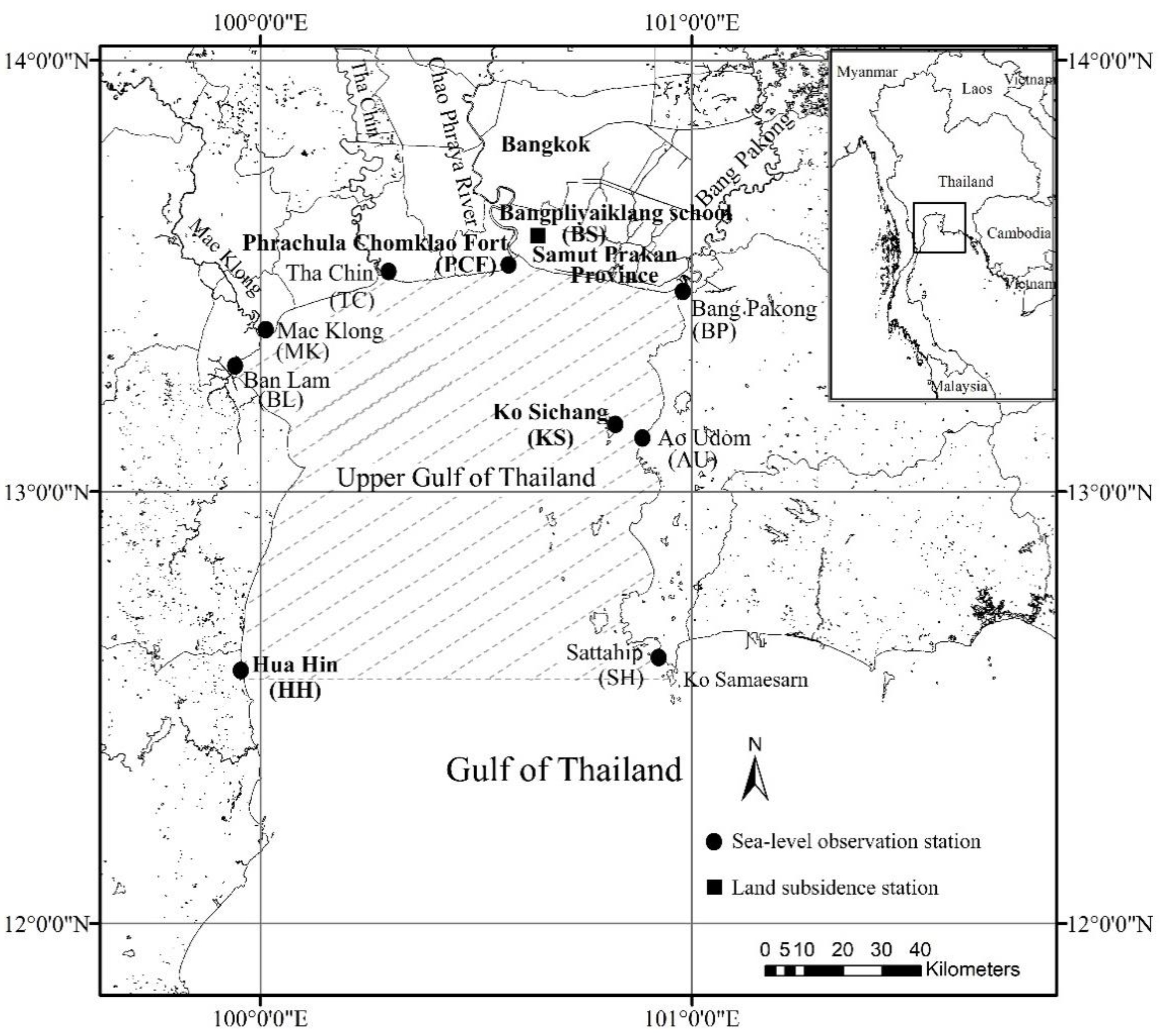
2.1. Study Area
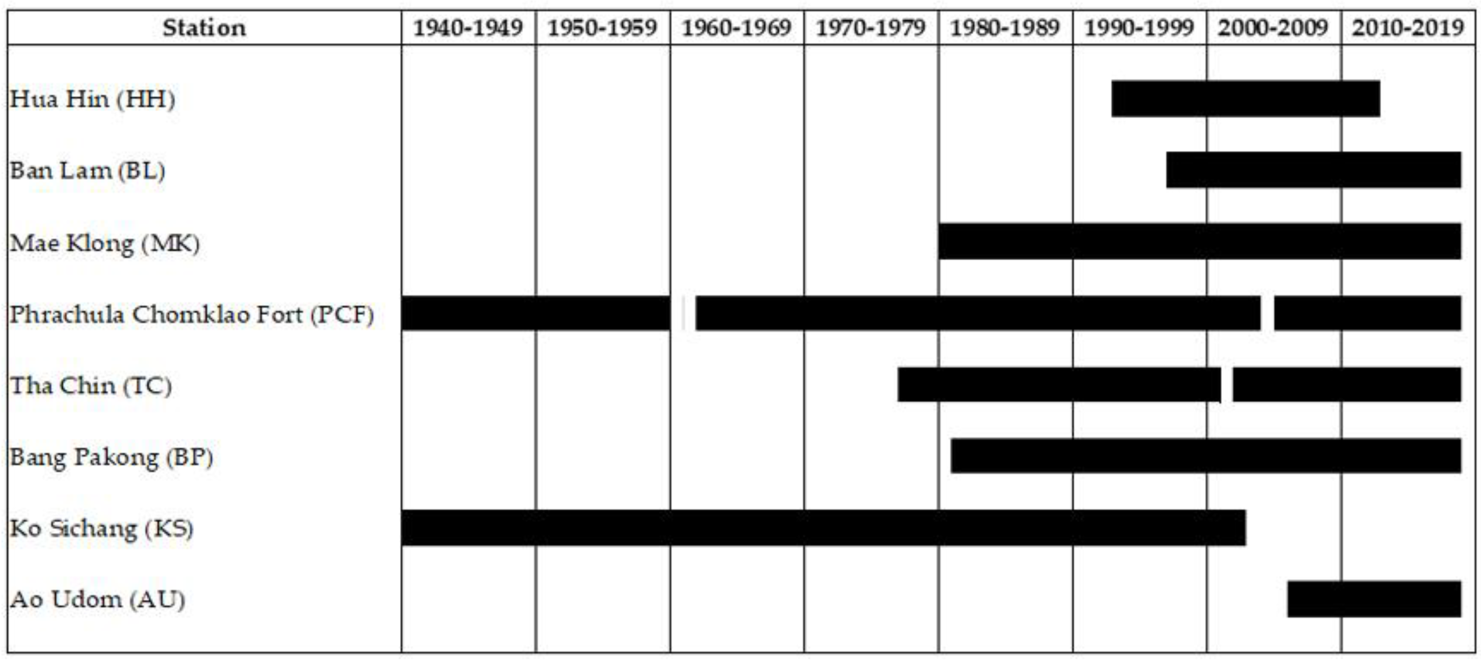
2.2. Data
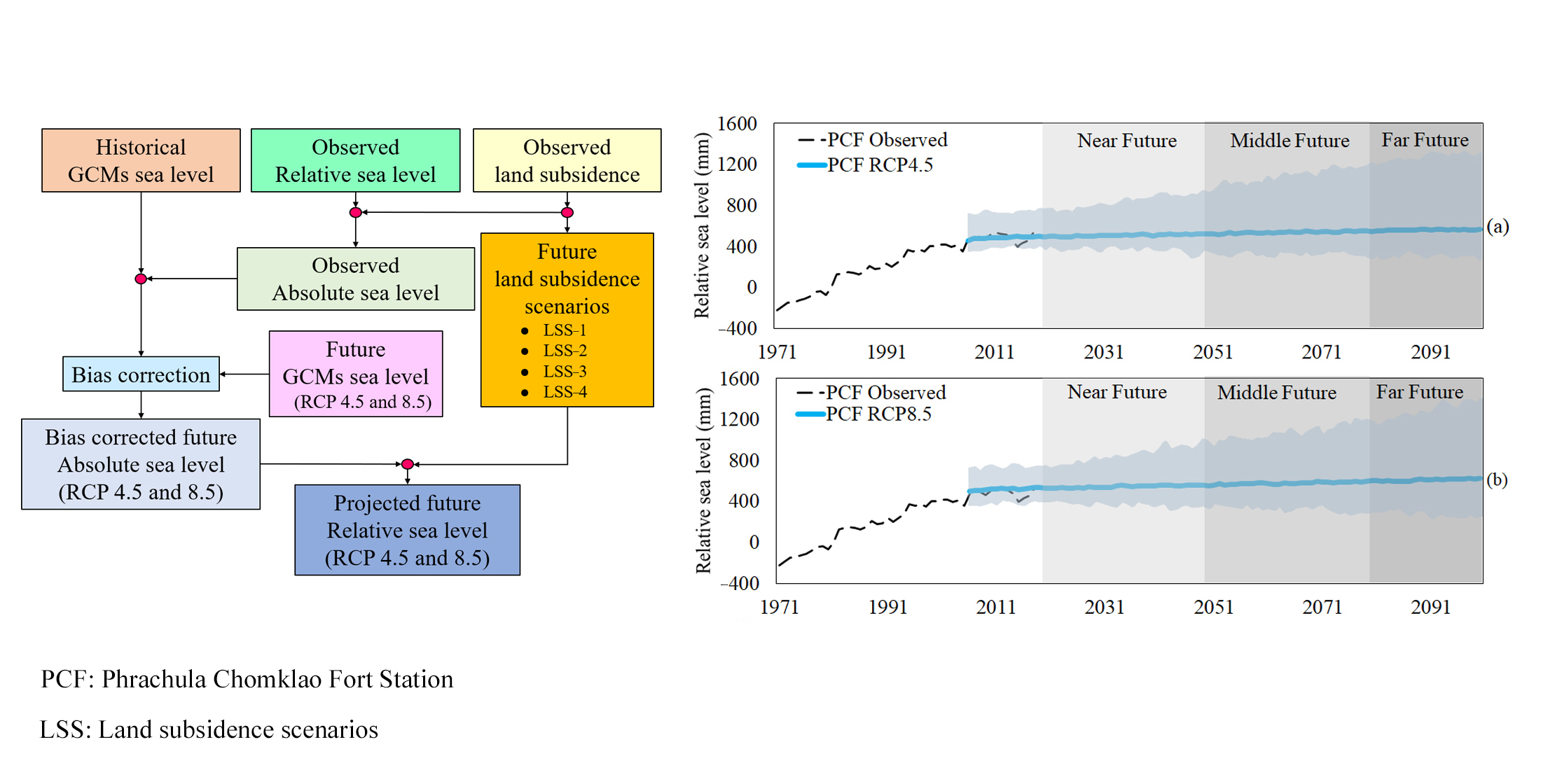
2.3. Methods
2.3.1. Observed Sea Level and Land Subsidence
2.3.2. Future Land Subsidence Scenario
2.3.3. Downscaling Sea Level
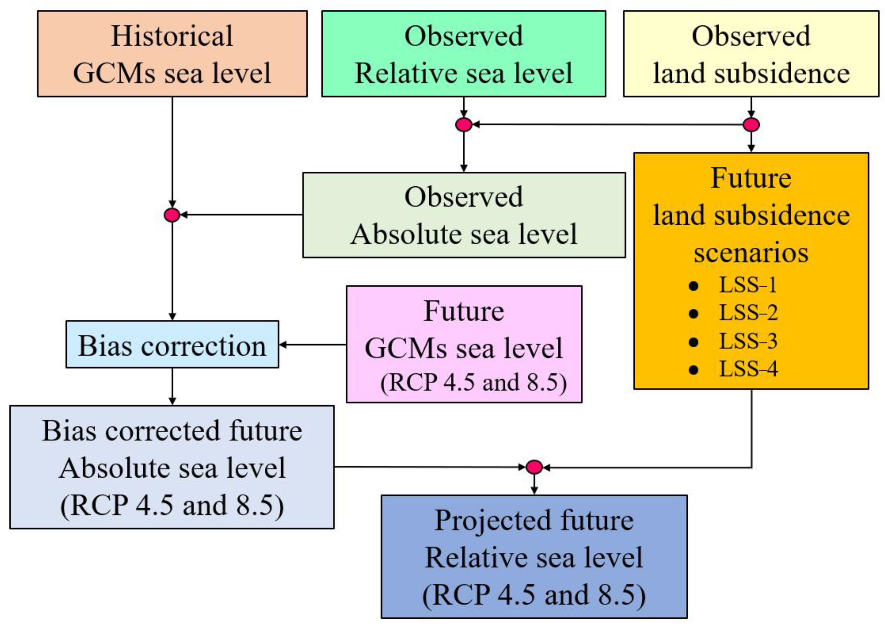
2.3.4. Projections of Sea Level
3. Results and Discussion
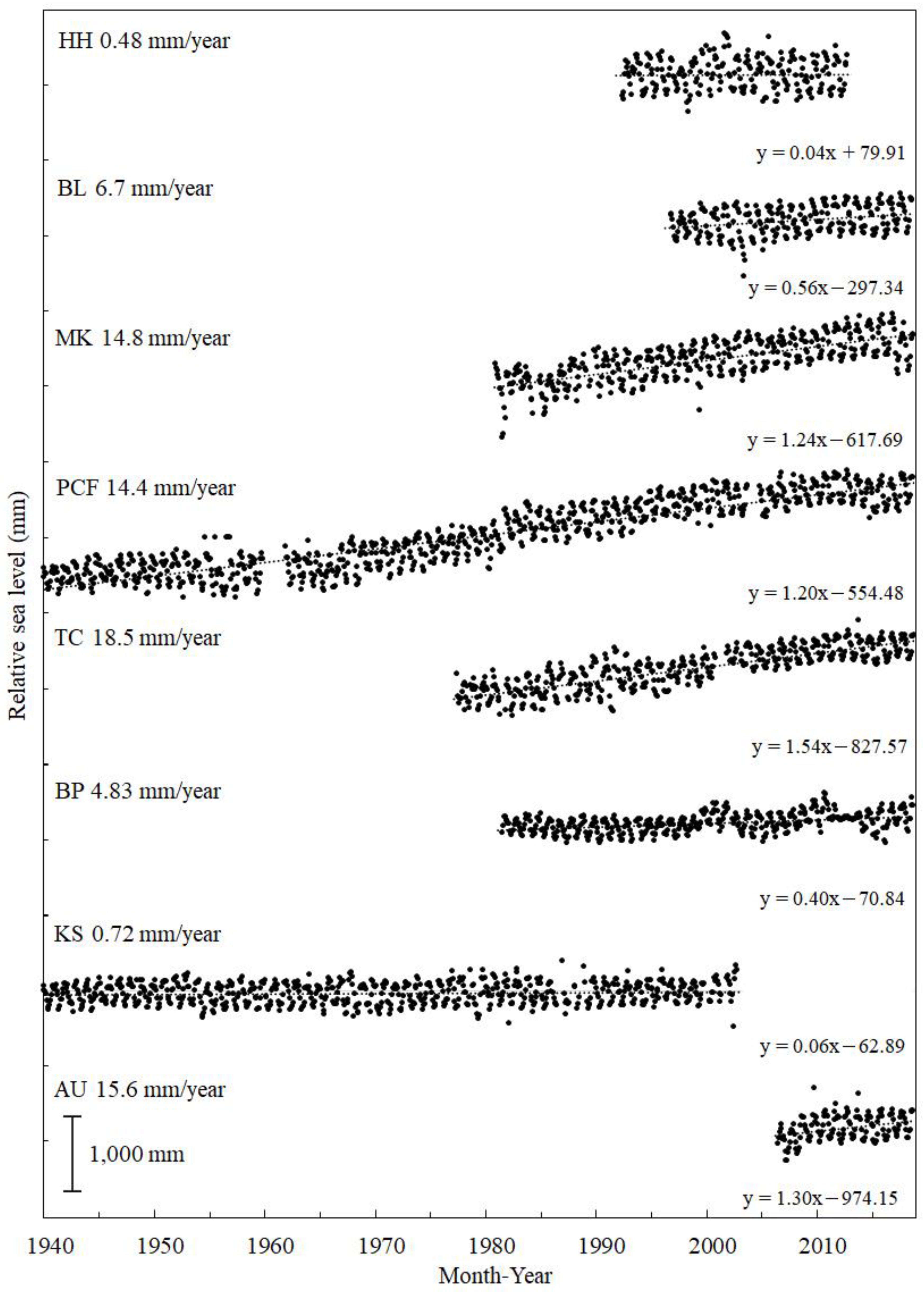
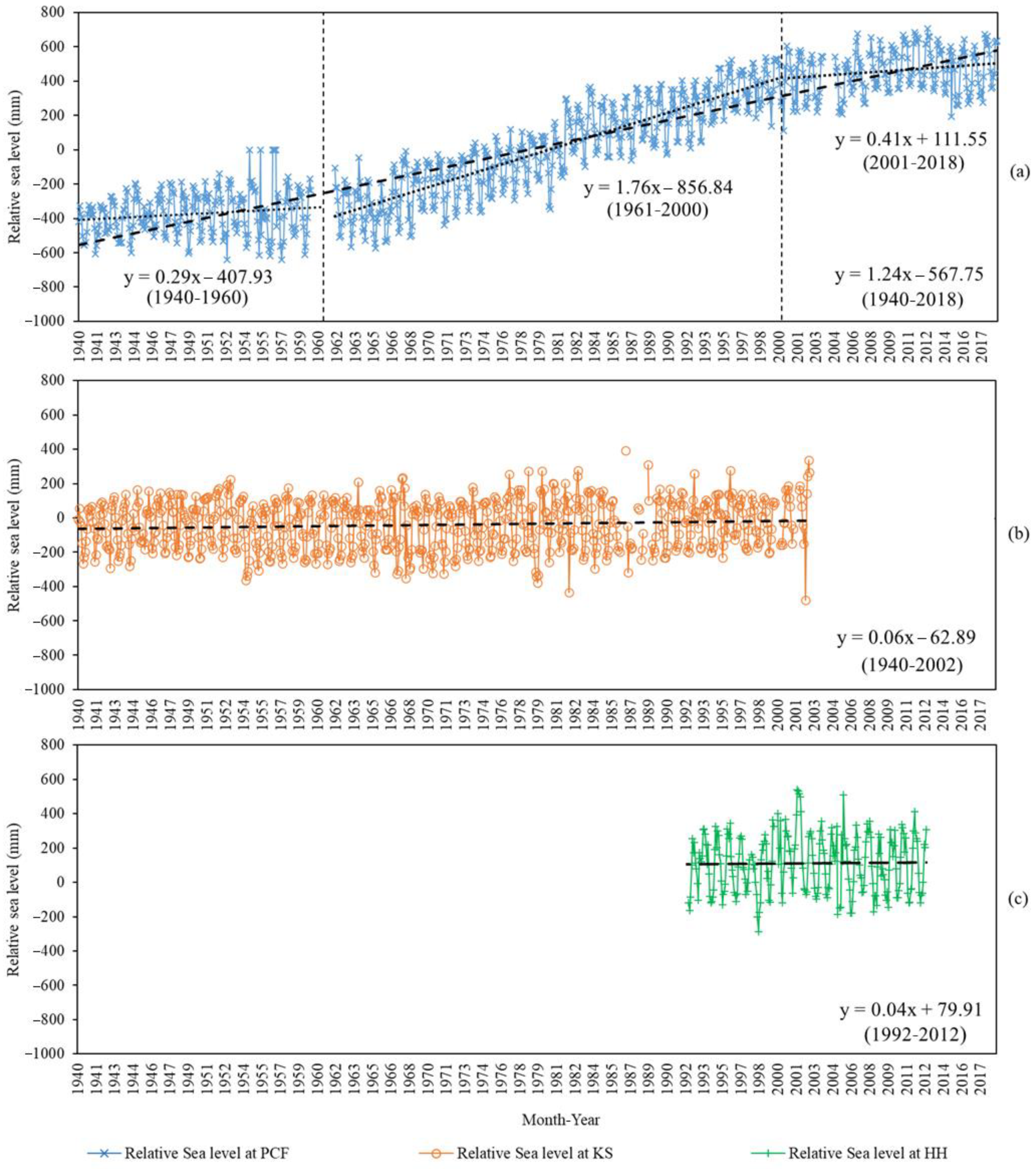
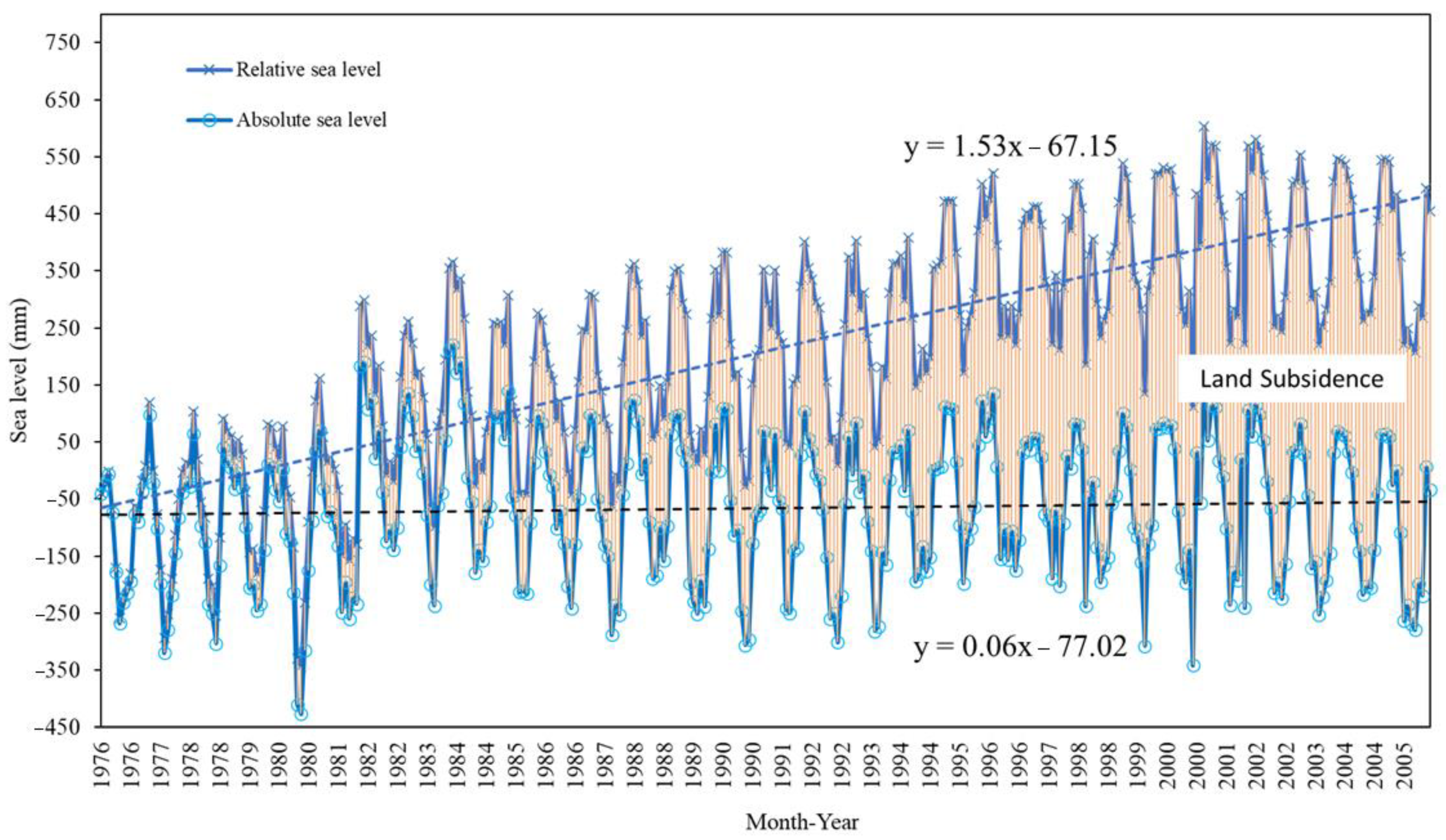
3.1. Analysis of Observed Sea Level
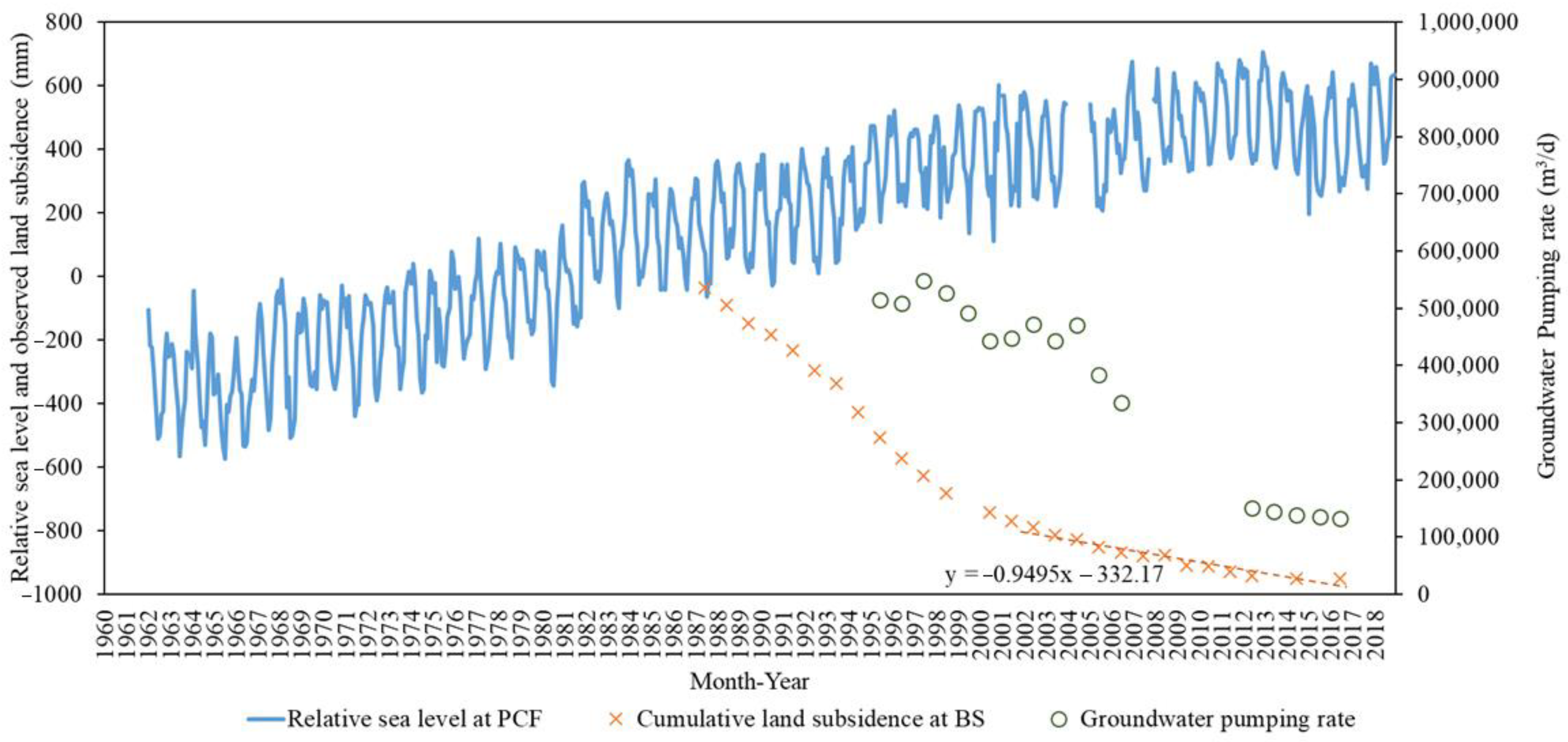
3.2. Groundwater Pumping and Land Subsidence
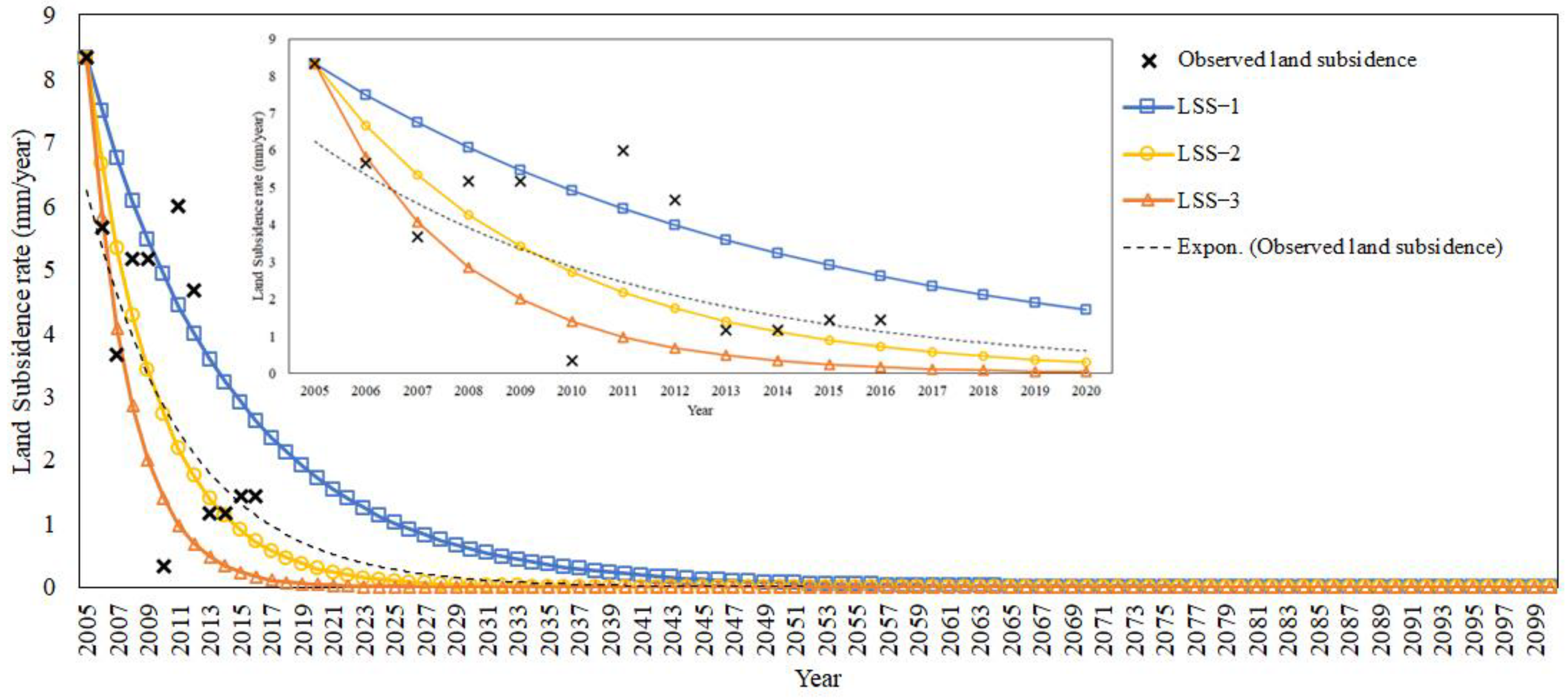
3.3. Future Land Subsidence Scenarios
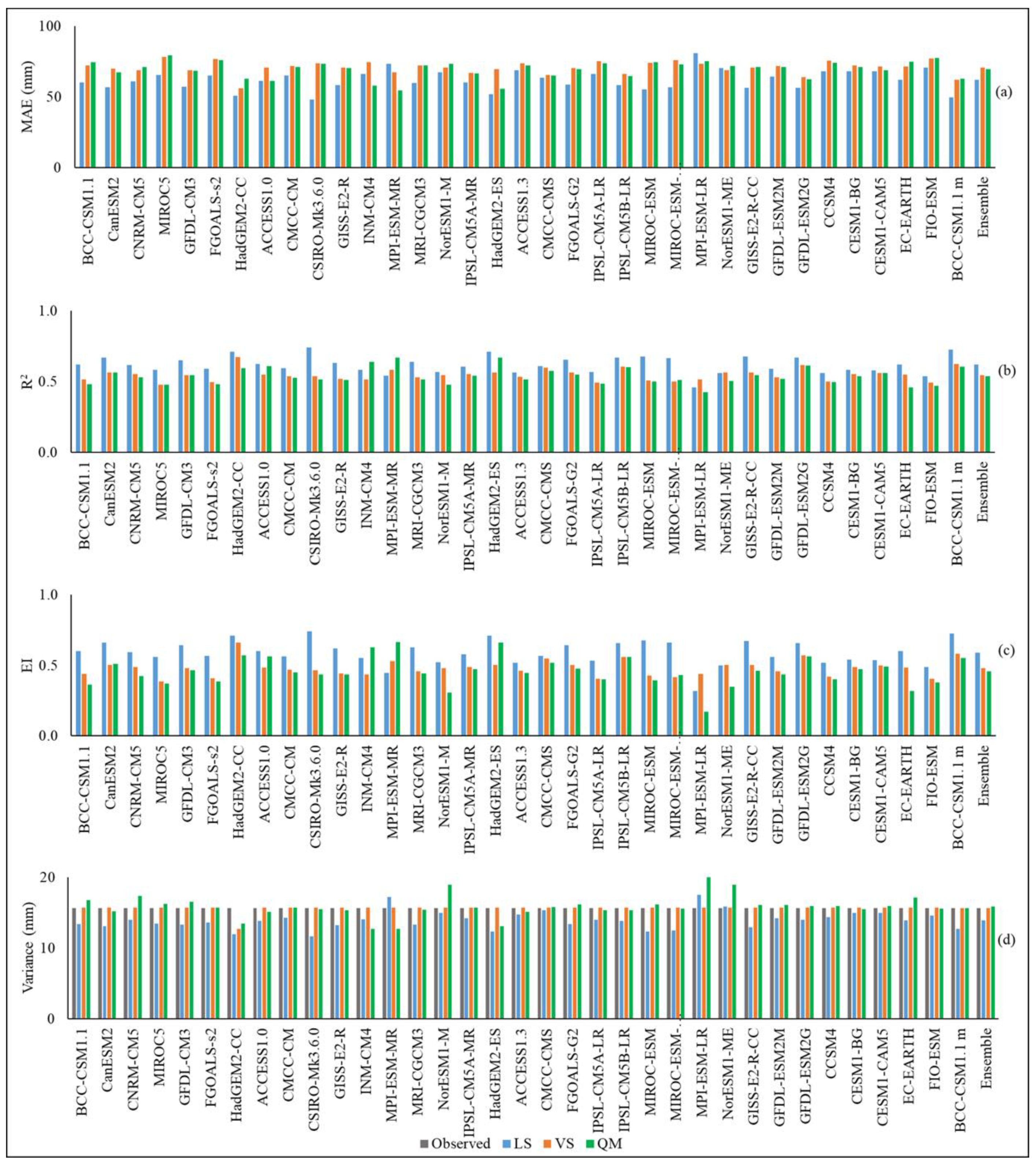
3.4. Bias Correction
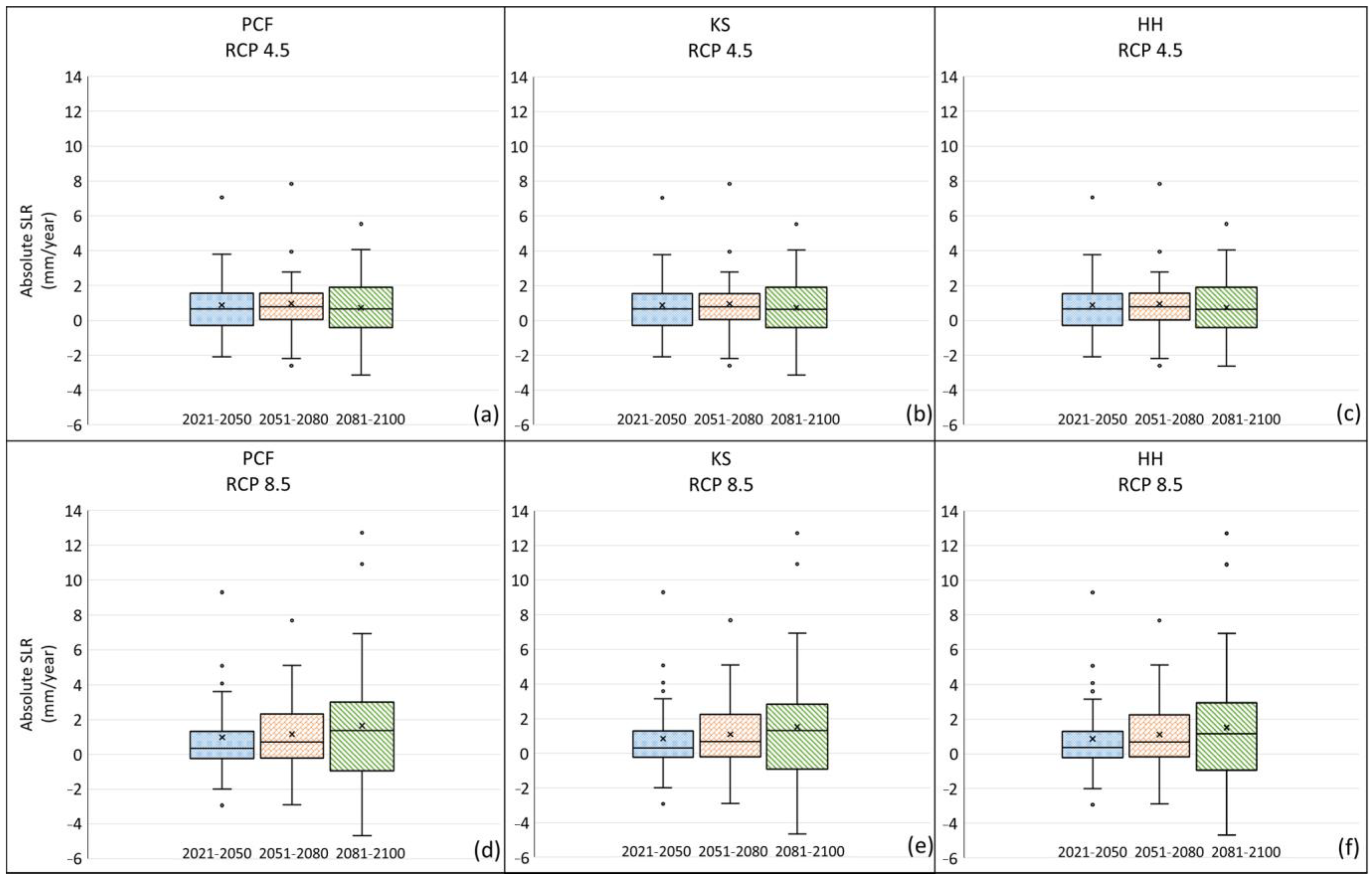
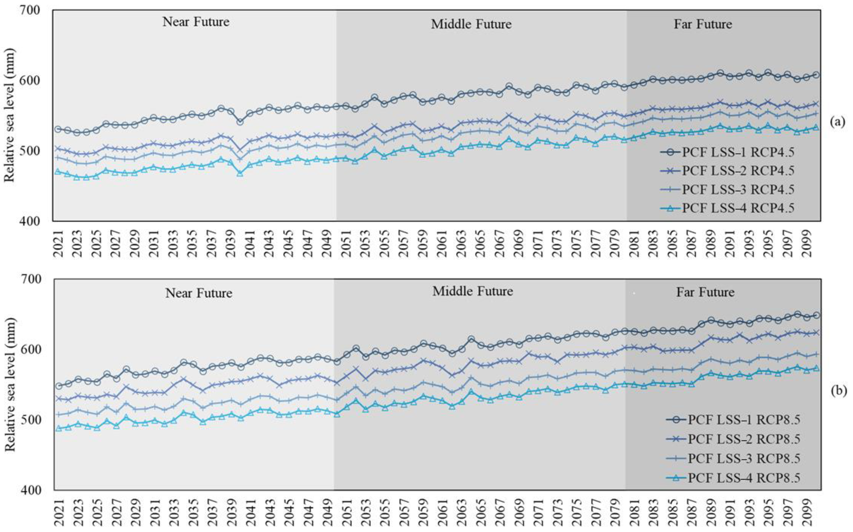
3.5. Sea Level Projections
4. Conclusions
Author Contributions
Funding
Institutional Review Board Statement
Informed Consent Statement
Data Availability Statement
Acknowledgments
Conflicts of Interest
References
- IPCC. Summary for Policymakers. In Global Warming of 1.5 °C. An IPCC Special Report; Delmotte, M., Zhai, P., Pörtner, H.-O., Roberts, D., Skea, J., Shukla, P.R., Pirani, A., Moufouma-Okia, W., Péan, C., Pidcock, R., et al., Eds.; World Meteorological Organization: Geneva, Switzerland, 2018; p. 32. [Google Scholar]
- IPCC. Summary for Policymakers. In Climate Change 2013: The Physical Science Basis. Contribution of Working Group I to the Fifth Assessment Report of the Intergovernmental Panel on Climate Change; Stocker, T.F., Qin, D., Plattner, G.-K., Tignor, M., Allen, S.K., Boschung, J., Nauels, A., Xia, Y., Bex, V., Midgley, P.M., Eds.; Cambridge University Press: Cambridge, UK, 2013; p. 1535. [Google Scholar]
- Church, J.A.; White, N.J. A 20th century acceleration in global sea-level rise. Geophys. Res. Lett. 2006, 33. [Google Scholar] [CrossRef]
- Dangendorf, S.; Hay, C.; Calafat, F.M.; Marcos, M.; Piecuch, C.G.; Berk, K.; Jensen, J. Persistent acceleration in global sea-level rise since the 1960s. Nat. Clim. Chang. 2019, 9, 705–710. [Google Scholar] [CrossRef]
- Hong, B.; Shen, J. Responses of estuarine salinity and transport processes to potential future sea-level rise in the Chesapeake Bay. Estuar. Coast. Shelf Sci. 2012, 104, 33–45. [Google Scholar] [CrossRef]
- Huang, W.; Foo, S. Neural network modeling of salinity variation in Apalachicola River. Water Res. 2002, 36, 356–362. [Google Scholar] [CrossRef]
- Bhuiyan, M.J.A.N.; Dutta, D. Assessing impacts of sea level rise on river salinity in the Gorai river network, Bangladesh. Estuar. Coast. Shelf Sci. 2012, 96, 219–227. [Google Scholar] [CrossRef]
- Suen, J.-P.; Lai, H.-N. A salinity projection model for determining impacts of climate change on river ecosystems in Taiwan. J. Hydrol. 2013, 493, 124–131. [Google Scholar] [CrossRef]
- Phien-wej, N.; Giao, P.; Nutalaya, N. Land subsidence in Bangkok, Thailand. Eng. Geol. 2006, 82, 187–201. [Google Scholar] [CrossRef]
- Ferguson, G.; Gleeson, T. Vulnerability of coastal aquifers to groundwater use and climate change. Nat. Clim. Chang. 2012, 2, 342–345. [Google Scholar] [CrossRef]
- Liu, Y.; Li, J.; Fasullo, J.; Galloway, D.L. Land subsidence contributions to relative sea level rise at tide gauge Galveston Pier 21, Texas. Sci. Rep. 2020, 10, 17905. [Google Scholar] [CrossRef] [PubMed]
- Saramul, S.; Ezer, T. Spatial variations of sea level along the coast of Thailand: Impacts of extreme land subsidence, earthquakes and the seasonal monsoon. Glob. Planet. Chang. 2014, 122, 70–81. [Google Scholar] [CrossRef]
- Nerem, R.S.; Beckley, B.D.; Fasullo, J.T.; Hamlington, B.D.; Masters, D.; Mitchum, G.T. Climate-change-driven accelerated sea-level rise detected in the altimeter era. Proc. Natl. Acad. Sci. USA 2018, 115, 2022–2025. [Google Scholar] [CrossRef] [PubMed]
- Slangen, A.B.A.; Carson, M.; Katsman, C.A.; van de Wal, R.S.W.; Köhl, A.; Vermeersen, L.L.A.; Stammer, D. Projecting twenty-first century regional sea-level changes. Clim. Chang. 2014, 124, 317–332. [Google Scholar] [CrossRef]
- Tessler, Z.D.; Vörösmarty, C.J.; Overeem, I.; Syvitski, J.P.M. A model of water and sediment balance as determinants of relative sea level rise in contemporary and future deltas. Geomorphology 2018, 305, 209–220. [Google Scholar] [CrossRef]
- Lorphensri, O.; Ladawadee, A.; Dhammasarn, S. Review of Groundwater Management and Land Subsidence in Bangkok, Thailand. In Groundwater and Subsurface Environments: Human Impacts in Asian Coastal Cities; Taniguchi, M., Ed.; Springer: Tokyo, Japan, 2011; pp. 127–142. ISBN 978-443-153-903-2. [Google Scholar]
- Minderhoud, P.S.J.; Erkens, G.; Pham, V.H.; Bui, V.T.; Erban, L.; Kooi, H.; Stouthamer, E. Impacts of 25 years of groundwater extraction on subsidence in the Mekong delta, Vietnam. Environ. Res. Lett. 2017, 12, 064006. [Google Scholar] [CrossRef] [PubMed]
- Trisirisatayawong, I.; Naeije, M.; Simons, W.; Fenoglio-Marc, L. Sea level change in the Gulf of Thailand from GPS-corrected tide gauge data and multi-satellite altimetry. Glob. Planet. Chang. 2011, 76, 137–151. [Google Scholar] [CrossRef]
- Kulp, S.A.; Strauss, B.H. New elevation data triple estimates of global vulnerability to sea-level rise and coastal flooding. Nat. Commun. 2019, 10, 4844. [Google Scholar] [CrossRef]
- Buranapratheprat, A.; Luadnakrob, P.; Yanagi, T.; Morimoto, A.; Qiao, F. The modification of water column conditions in the Gulf of Thailand by the influences of the South China Sea and monsoonal winds. Cont. Shelf Res. 2016, 118, 100–110. [Google Scholar] [CrossRef]
- Suwanlertcharoen, T.; Prukpitikul, S. Detection of Phytoplankton Blooms in the Upper Gulf of Thailand Using Sentinel-3A OLCI Imagery. Environ. Nat. Resour. J. 2018, 16, 9–20. [Google Scholar] [CrossRef]
- Yu, X.; Guo, X.; Morimoto, A.; Buranapratheprat, A. Simulation of river plume behaviors in a tropical region: Case study of the Upper Gulf of Thailand. Cont. Shelf Res. 2018, 153, 16–29. [Google Scholar] [CrossRef]
- ESGF Node at DKRZ. Available online: https://esgf-data.dkrz.de/projects/esgf-dkrz/ (accessed on 22 October 2020).
- Hayashi, T.; Tokunaga, T.; Aichi, M.; Shimada, J.; Taniguchi, M. Effects of human activities and urbanization on groundwater environments: An example from the aquifer system of Tokyo and the surrounding area. Sci. Total Environ. 2009, 407, 3165–3172. [Google Scholar] [CrossRef] [PubMed]
- Sato, C.; Haga, M.; Nishino, J. Land subsidence and groundwater management in Tokyo. Intern. Rev. Environ. Strateg. 2006, 6, 403–424. [Google Scholar]
- Qin, H.; Andrews, C.B.; Tian, F.; Cao, G.; Luo, Y.; Liu, J.; Zheng, C. Groundwater-pumping optimization for land-subsidence control in Beijing plain, China. Hydrogeol. J. 2018, 26, 1061–1081. [Google Scholar] [CrossRef]
- Piani, C.; Haerter, J.O.; Coppola, E. Statistical bias correction for daily precipitation in regional climate models over Europe. Theor. Appl. Climatol. 2010, 99, 187–192. [Google Scholar] [CrossRef]
- Mahmood, R.; Jia, S. An extended linear scaling method for downscaling temperature and its implication in the Jhelum River basin, Pakistan, and India, using CMIP5 GCMs. Theor. Appl. Climatol. 2017, 130, 725–734. [Google Scholar] [CrossRef]
- Maurer, E.P.; Pierce, D.W. Bias correction can modify climate model simulated precipitation changes without adverse effect on the ensemble mean. Hydrol. Earth Syst. Sci. 2014, 18, 915–925. [Google Scholar] [CrossRef]
- Nguyen, H.; Mehrotra, R.; Sharma, A. Can the variability in precipitation simulations across GCMs be reduced through sensible bias correction? Clim. Dyn. 2017, 49, 3257–3275. [Google Scholar] [CrossRef]
- Prasanna, V. Statistical bias correction method applied on CMIP5 datasets over the Indian region during the summer monsoon season for climate change applications. Theor. Appl. Climatol. 2018, 131, 471–488. [Google Scholar] [CrossRef]
- Um, M.-J.; Kim, H.; Heo, J.-H. Hybrid approach in statistical bias correction of projected precipitation for the frequency analysis of extreme events. Adv. Water Resour. 2016, 94, 278–290. [Google Scholar] [CrossRef]
- Nahar, J.; Johnson, F.; Sharma, A. Assessing the extent of non-stationary biases in GCMs. J. Hydrol. 2017, 549, 148–162. [Google Scholar] [CrossRef]
- Lenderink, G.; Buishand, A.; van Deursen, W. Estimates of future discharges of the river Rhine using two scenario methodologies: Direct versus delta approach. Hydrol. Earth Syst. Sci. 2007, 11, 1145–1159. [Google Scholar] [CrossRef]
- Fang, G.H.; Yang, J.; Chen, Y.N.; Zammit, C. Comparing bias correction methods in downscaling meteorological variables for a hydrologic impact study in an arid area in China. Hydrol. Earth Syst. Sci. 2015, 19, 2547–2559. [Google Scholar] [CrossRef]
- Teutschbein, C.; Seibert, J. Bias correction of regional climate model simulations for hydrological climate-change impact studies: Review and evaluation of different methods. J. Hydrol. 2012, 456–457, 12–29. [Google Scholar] [CrossRef]
- Terink, W.; Hurkmans, R.T.W.L.; Torfs, P.J.J.F.; Uijlenhoet, R. Evaluation of a bias correction method applied to downscaled precipitation and temperature reanalysis data for the Rhine basin. Hydrol. Earth Syst. Sci. 2010, 14, 687–703. [Google Scholar] [CrossRef]
- Themeßl, M.J.; Gobiet, A.; Leuprecht, A. Empirical-statistical downscaling and error correction of daily precipitation from regional climate models. Int. J. Climatol. 2011, 31, 1530–1544. [Google Scholar] [CrossRef]
- Panofsky, H.A.; Brier, G.W. Some Applications of Statistics to Meteorology.; The Pennsylvania State University Press: Philadelphia, PA, USA, 1958. [Google Scholar]
- Babel, M.S.; Gupta, A.D.; Sto. Domingo, N.D. Groundwater Resource Management in Bangkok. In Sustainable Groundwater Management in Asian Cities: A Summary Report of Research on Sustainable Water Management in Asia; Institute for Global Environmental Strategies: Kanagawa, Japan, 2006; pp. 71–80. Available online: http://www.jstor.org/stable/resrep00865.19 (accessed on 30 April 2021).
- Babel, M.S.; Rivas, A.A.; Gupta, A.D.; Kataoka, Y. Improving Groundwater Quality Management for the Sustainable Utilization of the Bangkok Aquifer System. Int. J. Water Resour. Dev. 2012, 28, 355–371. [Google Scholar] [CrossRef]
- Vongvisessomjai, S. Will sea-level really fall in the Gulf of Thailand? Songklanakarin J. Sci. Technol. 2006, 28, 227–248. [Google Scholar]
- Babel, M.S.; Gupta, A.D.; Sto. Domingo, N.D. Land subsidence: A consequence of groundwater exploitation in Bangkok, Thailand. Int. Rev. Environ. Strateg. 2006, 6, 307–328. [Google Scholar]


| Data/Station | Location | Frequency | Data Period | Remarks | |
|---|---|---|---|---|---|
| Lat | Long | ||||
| Sea level | |||||
| Hua Hin (HH) | 12°34′22″ N | 99°57′48″ E | Monthly | 1992–2012 | |
| Ban Lam (BL) | 13°15′47″ N | 99°56′44″ E | Monthly | 1997–2018 | |
| Mae Klong (MK) | 13°22′36″ N | 99°59′44″ E | Monthly | 1980–2018 | |
| Phrachula Chomklao Fort (PCF) | 13°33′06″ N | 100°34′44″ E | Monthly | 1940–2018 | Data missing for 1960, 1961 and 2004 |
| Tha Chin (TC) | 13°30′36″ N | 100°16′40″ E | Monthly | 1977–2018 | Data missing for 2001 |
| Bang Pakong (BP) | 13°29′00″ N | 101°00′23″ E | Monthly | 1981–2018 | |
| Ko Sichang (KS) | 13°09′00″ N | 100°49′00″ E | Monthly | 1940–2002 | |
| Ao Udom (AU) | 13°07′25″ N | 100°53′46″ E | Monthly | 2006–2018 | |
| Land subsidence | |||||
| Bangpliyaiklang School (BS) | 13°36′27″ N | 100°42′12″ E | Annual | 1987–2016 | Data missing for 1999, 2013, and 2015 |
| Groundwater pumping | Samut Prakan province | Annual | 1996–2006; 2012–2016 | ||
| Model | Modeling Center | Atmospheric (AGCM) Grid Resolution | Oceanic (OGCM) Grid Resolution | Vintage |
|---|---|---|---|---|
| ACCESS1.0 | CSIRO-BOM, Australia | 192 × 145L38 | 360 × 300L50 | 2011 |
| ACCESS1.3 | CSIRO-BOM, Australia | 192 × 145L38 | 360 × 300L50 | 2011 |
| BCC-CSM1.1 | BCC, China | 128 × 64L26 | 360 × 232L40 | 2011 |
| BCC-CSM1.1(m) | BCC, China | 320 × 160L26 | 360 × 232L40 | 2011 |
| CanESM2 | CCCma, Canada | 128 × 64L35 | 256 × 192L40 | 2010 |
| CCSM4 | NCAR, USA | 288 × 192L26 | 320 × 384L60 | 2010 |
| CESM1(BGC) | NCAR, USA | 288 × 192L26 | 320 × 384L60 | 2010 |
| CESM1(CAM5) | NCAR, USA | 288 × 192L26 | 320 × 384L60 | 2010 |
| CMCC-CM | CMCC, Italy | 480 × 240L31 | 182 × 149L31 | 2009 |
| CMCC-CMS | CMCC, Italy | 192 × 96L95 | 182 × 149L31 | 2009 |
| CNRM-CM5 | CNRM-CERFACS, France | 256 × 128L31 | 362 × 292L42 | 2010 |
| CSIRO-Mk3.6.0 | CSIRO-QCCCE, Australia | 192 × 96L18 | 192 × 189L31 | 2009 |
| EC-EARTH | EC-Earth consortium, Netherland | 320 × 160L26 | 362 × 292L30 | 2010 |
| FGOALS-g2 | LASG-IAP, China | 128 × 60L26 | 360 × 196L30 | 2011 |
| FGOALS-s2 | LASG-IAP, China | 128 × 108L26 | 360 × 196L30 | 2011 |
| FIO-ESM | FIO, SOA, China | 128 × 64L26 | 327 × 300L40 | 2011 |
| GFDL-CM3 | NOAA GFDL, USA | 144 × 90L48 | 360 × 200L50 | 2011 |
| GFDL-ESM2G | NOAA GFDL, USA | 144 × 90L24 | 360 × 210L63 | 2012 |
| GFDL-ESM2M | NOAA GFDL, USA | 144 × 90L24 | 360 × 200L50 | 2011 |
| GISS-E2-R | NASA GISS, USA | 144 × 90L40 | 288 × 180L32 | 2011 |
| GISS-E2-R-CC | NASA GISS, USA | 144 × 90L40 | 288 × 180L32 | 2011 |
| HadGEM2-CC | MOHC, UK | 192 × 145L60 | 360 × 216L40 | 2010 |
| HadGEM2-ES | MOHC, UK | 192 × 145L38 | 360 × 216L40 | 2009 |
| INM-CM4 | INM, Russia | 180 × 120L21 | 360 × 340L40 | 2009 |
| IPSL-CM5A-LR | IPSL, France | 96 × 96L39 | 182 × 149L31 | 2009 |
| IPSL-CM5A-MR | IPSL, France | 143 × 144L39 | 182 × 149L31 | 2009 |
| IPSL-CM5B-LR | IPSL, France | 96 × 96L39 | 182 × 149L31 | 2009 |
| MIROC-ESM | MIROC, Japan | 128 × 64L80 | 256 × 192L44 | 2010 |
| MIROC-ESM-CHEM | MIROC, Japan | 128 × 64L80 | 256 × 192L44 | 2010 |
| MIROC5 | MIROC, Japan | 256 × 128L40 | 256 × 224L50 | 2010 |
| MPI-ESM-LR | MPI-M, Germany | 192 × 96L47 | 256 × 220L40 | 2009 |
| MPI-ESM-MR | MPI-M, Norway | 192 × 96L95 | 802 × 404L40 | 2009 |
| MRI-CGCM3 | MRI, Japan | 320 × 160L48 | 360 × 368L51 | 2011 |
| NorESM1-M | NCC, Norway | 144 × 96L26 | 320 × 384L53 | 2011 |
| NorESM1-ME | NCC, Norway | 144 × 96L26 | 320 × 384L53 | 2012 |
| Station | Rate of Relative SLR (mm/Year) | LSS | Projected Rate of Relative SLR (mm/Year) | |||||||||
|---|---|---|---|---|---|---|---|---|---|---|---|---|
| Observed | Scenario | RCP4.5 | RCP8.5 | |||||||||
| 1940–2018 | 1940–2002 | 1992–2012 | Near Future | Mid-Future | Far Future | Long-Term | Near Future | Mid-Future | Far Future | Long-Term | ||
| 2021–2050 | 2051–2080 | 2081–2100 | 2021–2100 | 2021–2050 | 2051–2080 | 2081–2100 | 2021–2100 | |||||
| PCF | 14.98 | - | - | LSS-1 | 1.29 | 0.96 | 0.71 | 1.05 | 1.27 | 1.11 | 1.51 | 1.18 |
| LSS-2 | 0.89 | 0.94 | 0.71 | 0.95 | 0.87 | 1.09 | 1.51 | 1.07 | ||||
| LSS-3 | 0.86 | 0.94 | 0.71 | 0.94 | 0.85 | 1.09 | 1.51 | 1.07 | ||||
| LSS-4 | 0.86 | 0.94 | 0.71 | 0.94 | 0.85 | 1.09 | 1.51 | 1.07 | ||||
| KS | - | 0.75 | - | - | 0.86 | 0.94 | 0.71 | 0.94 | 0.85 | 1.09 | 1.51 | 1.07 |
| HH | - | - | 0.48 | - | 0.87 | 0.94 | 0.73 | 0.95 | 0.86 | 1.10 | 1.52 | 1.08 |
| Station | Land Subsidence Scenario | RCP4.5 | RCP8.5 | |||||||
|---|---|---|---|---|---|---|---|---|---|---|
| 2021–2050 | 2051–2080 | 2081–2100 | 2021–2100 | 2021–2050 | 2051–2080 | 2081–2100 | 2021–2100 | |||
| Cumulative Relative SLR | Cumulative Relative SLR | |||||||||
| PCF | LSS-1 | max | 223.93 | 235.48 | 105.04 | 624.41 | 291.42 | 230.56 | 241.56 | 632.60 |
| mean | 38.59 | 28.86 | 13.50 | 82.92 | 38.23 | 33.29 | 28.78 | 93.01 | ||
| min | −50.51 | −77.80 | −59.98 | −86.63 | −75.42 | −86.49 | −88.79 | −127.24 | ||
| LSS-2 | max | 211.91 | 234.94 | 105.02 | 616.33 | 279.41 | 230.02 | 241.54 | 624.52 | |
| mean | 26.57 | 28.32 | 13.48 | 74.83 | 26.22 | 32.75 | 28.76 | 84.91 | ||
| min | −62.52 | −78.34 | −60.00 | −94.70 | −87.43 | −87.03 | −88.82 | −135.32 | ||
| LSS-3 | max | 211.22 | 234.94 | 105.02 | 616.00 | 278.71 | 230.02 | 241.54 | 624.18 | |
| mean | 25.88 | 28.32 | 13.48 | 74.49 | 25.52 | 32.75 | 28.76 | 84.57 | ||
| min | −63.22 | −78.34 | −60.00 | −95.04 | −88.12 | −87.03 | −88.82 | −135.65 | ||
| LSS-4 | max | 211.18 | 234.94 | 105.02 | 615.98 | 278.67 | 230.02 | 241.54 | 624.16 | |
| mean | 25.84 | 28.32 | 13.48 | 74.47 | 25.48 | 32.75 | 28.76 | 84.56 | ||
| min | −63.26 | −78.34 | −60.00 | −95.06 | −88.16 | −87.03 | −88.82 | −135.67 | ||
| KS | - | max | 211.18 | 234.94 | 105.02 | 615.98 | 278.67 | 230.02 | 241.54 | 624.16 |
| mean | 25.90 | 28.14 | 13.48 | 74.41 | 25.44 | 32.80 | 28.78 | 84.56 | ||
| min | −63.26 | −78.34 | −60.00 | −95.06 | −88.16 | −87.03 | −88.82 | −135.67 | ||
| HH | - | max | 211.18 | 234.94 | 105.02 | 615.98 | 278.67 | 230.02 | 241.54 | 624.16 |
| mean | 26.00 | 28.18 | 13.84 | 74.88 | 25.71 | 32.93 | 28.94 | 84.98 | ||
| min | −63.26 | −78.34 | −50.07 | −95.06 | −88.16 | −87.03 | −88.82 | −135.67 | ||
Publisher’s Note: MDPI stays neutral with regard to jurisdictional claims in published maps and institutional affiliations. |
© 2021 by the authors. Licensee MDPI, Basel, Switzerland. This article is an open access article distributed under the terms and conditions of the Creative Commons Attribution (CC BY) license (https://creativecommons.org/licenses/by/4.0/).
Share and Cite
Jaroenongard, C.; Babel, M.S.; Shrestha, S.; Weesakul, S.; Nitivattananon, V.; Khadka, D. Projecting Relative Sea Level Rise under Climate Change at the Phrachula Chomklao Fort Tide Gauge in the Upper Gulf of Thailand. Water 2021, 13, 1702. https://doi.org/10.3390/w13121702
Jaroenongard C, Babel MS, Shrestha S, Weesakul S, Nitivattananon V, Khadka D. Projecting Relative Sea Level Rise under Climate Change at the Phrachula Chomklao Fort Tide Gauge in the Upper Gulf of Thailand. Water. 2021; 13(12):1702. https://doi.org/10.3390/w13121702
Chicago/Turabian StyleJaroenongard, Chirayu, Mukand S. Babel, Sangam Shrestha, Sutat Weesakul, Vilas Nitivattananon, and Dibesh Khadka. 2021. "Projecting Relative Sea Level Rise under Climate Change at the Phrachula Chomklao Fort Tide Gauge in the Upper Gulf of Thailand" Water 13, no. 12: 1702. https://doi.org/10.3390/w13121702
APA StyleJaroenongard, C., Babel, M. S., Shrestha, S., Weesakul, S., Nitivattananon, V., & Khadka, D. (2021). Projecting Relative Sea Level Rise under Climate Change at the Phrachula Chomklao Fort Tide Gauge in the Upper Gulf of Thailand. Water, 13(12), 1702. https://doi.org/10.3390/w13121702