Article

Copula-Based Infilling Methods for Daily Suspended Sediment Loads

Department of Hydraulic and Ocean Engineering, National Cheng Kung University, Tainan 701, Taiwan
*
Author to whom correspondence should be addressed.
Water 2021, 13(12), 1701; https://doi.org/10.3390/w13121701
Submission received: 4 May 2021 / Revised: 10 June 2021 / Accepted: 16 June 2021 / Published: 19 June 2021
(This article belongs to the Section Hydrology)

Abstract

:
Less-frequent and inadequate sampling of sediment data has negatively impacted the long and continuous records required for the design and operation of hydraulic facilities. This data-scarcity problem is often found in most river basins of Taiwan. This study aims to propose a parsimonious probabilistic model based on copulas to infill daily suspended sediment loads using streamflow discharge. A copula-based bivariate distribution model of sediment and discharge of the paired recorded data is constructed first. The conditional distribution of sediment load given observed discharge is used to provide probabilistic estimation of sediment loads. In addition, four different methods based on the derived conditional distribution of sediment load are used to give single-value estimations. The obtained outcomes of these methods associated with the results of the traditional sediment rating curve are compared with recorded data and evaluated in terms of root mean square error (RMSE), mean absolute percentage error (MAPE), Nash-Sutcliffe efficiency (NSE), and modified Nash-Sutcliffe efficiency (MNSE). The proposed approach is applied to the Janshou station located in eastern Taiwan with recorded daily data for the period of 1960–2019. The results indicate that the infilled sediments by the sediment rating curve exhibit better performance in RMSE and NSE, while the copula-based methods outperform in MAPE and MNSE. Additionally, the infilled sediments by the copula-based methods preserve scattered characteristics of observed sediment-discharge relationships and exhibit similar frequency distributions to that of recorded sediment data.

1. Introduction

Hydrologic and climate data play a significant role in water-resources engineering planning, design, and management. Sufficiently long and complete data are essential for providing accurate statistical analysis in design and establishing efficient operation rules of hydraulic facilities. Hydrologic and climate data are uniquely recorded in time and space. If the data are not recorded at a specific time and location, the lost values can only be estimated [1]. Incomplete and missing data are frequently met in many applications worldwide since a considerable amount factors lead to missing data. These factors include equipment failures, extreme natural disasters (e.g., typhoon, earthquake, and landslide), mishandling of recorded data, malfunction of data storage systems, and others [2,3]. Infilling the missing data has thus become a common practice when pre-processing data to provide long and complete data for optimal hydrologic modeling and design purposes.
Infilling or imputing missing data is a process of substituting the missing values with the most plausible values [4,5]. A vast amount of approaches such as linear regression, multiple linear regression, machine learning techniques, copula-based estimation, and others have been proposed in the literature to infill missing data. Bárdossy and Pegram [1], Ben Aissia et al. [3], and Hamzah et al. [6] provide detailed reviews on methods used in infilling missing hydrologic data.
Suspended sediment load is an important variable in water-resources engineering since it affects reservoir sedimentation, hydraulic structures design, water quality, ecological and recreation, watershed management, and channel stability [7,8]. In addition to missing data, infrequent or periodical sampling is another primary reason for incomplete sedimentation data in most river basins. Suspended sediment load transported in rivers is a complex process which relates to physical characteristics of watershed and rivers. Predicting sediment loads through physical models might be prohibitive due to the complex process and lack of long-term observations [9]. Instead, statistical empirical models serve as alternative approaches to infill missing or unrecorded (missing thereafter) sediment data since these models relax the requirement of detailed physical information. For example, the sediment rating curve based on the empirical relationship between suspended sediment load and streamflow discharge is traditionally used to infill missing sediment data since continuous discharge records are available in most river basins [10]. Several recent studies [11,12,13,14,15,16,17,18,19,20,21,22,23,24,25,26,27] have proposed various techniques or adopted various variables to estimate or predict suspended sediment loads. Ben Aissia et al. [3] indicated that the copula-based method is one of the recent methods and provides probabilistic characteristics of the missing data. Di Lascio et al. [5] revealed that Käärik and Käärik [4] firstly propose the Gaussian copula to impute correlated incomplete data.
Inherently scattered characteristics between observed suspended sediment load and streamflow discharge indicate that joint modeling of the probabilistic properties between suspended sediment loads and streamflow discharge is a proper approach to achieve this purpose. Difficulties in deriving such bivariate distribution of sediment load and discharge stem from different marginal distributions used to fit sediment load and discharge. Copulas have recently gained popularity worldwide [28,29,30,31,32,33,34,35,36,37,38,39,40,41,42,43,44,45,46,47] in hydrology as they construct a multivariate distribution by separately linking different marginal univariate distributions and the joint dependence structure among random variables. However, Zhang et al. [48] indicated that few studies use copulas to explore the joint distribution of sediment and discharge. The related studies include Bezak et al. [49], who conducted frequency analysis of annual peak discharge and the corresponding hydrograph volume and suspended sediment concentration from stations located in Slovenia and USA using trivariate symmetric and asymmetric copula functions. The authors of [48] constructed a bivariate probability distribution of annual runoff and sediment in the Wei River (China) using copulas for estimating synchronous-asynchronous encounter probabilities of annual rich-poor runoff and sediment. Guo et al. [50] used the double-mass-curve method to detect the inflection point in the runoff-sediment relationship of the Weihe River (China) and analyzed the synchronous-asynchronous joint properties of high-low runoff and sediment based on copulas. Bezak et al. [18] estimated event-based suspended sediment loads based on measured precipitation sums and discharge using copulas in two catchments of Slovenia. Huang et al. [51] used the copula-based method to detect the nonstationarity of the relationship between annual runoff and sediment load in the Wei River, China. Shojaeezadeh et al. [9] proposed a probabilistic method based on copulas with Bayesian networks to predict the suspended sediment load given discharge for high flow events in seven major rivers of the contiguous US. Peng et al. [52] simulated daily suspended sediment concentration through the copula-based multivariate conditional distribution using previous daily suspended sediment concentration and concurrent daily streamflow of the Jinsha River basin, China. Peng et al. [53] proposed a copula-based model of the annual maximum suspended sediment concentration, peak discharge, and flood volume and analyzed multivariate joint and conditional return periods for suspended sediment concentration under flood conditions in the Jinsha River basin, China.
The copula-based method infills the missing data by using the conditional distribution of missing variables given the value of observed variable, which describes possible outcomes of missing data associated with corresponding probabilities. However, single-value estimation of missing variable is often required in practical applications. Several approaches are proposed in the literature to estimate the single missing value by copula-based conditional distribution. Käärik and Käärik [4] suggested the most likely value (i.e., the mode) as the imputed value. Di Lascio et al. [5] obtained the single missing value by the Hit or Miss Monte Carlo method. Bezak et al. [18] suggested the median of 10,000 possible sediment values from the copula-based conditional distribution of 10,000 randomly generated peak discharge and precipitation. Peng et al. [52] proposed a stochastic simulation procedure to obtain the daily suspended sediment concentration using previous daily suspended sediment concentration and concurrent daily streamflow.
The main aim of this study is to infill daily suspended sediment loads based on copulas to provide probabilistic as well as single-value estimations using streamflow discharge. A copula-based bivariate probability model of concurrent daily suspended sediment load and discharge is firstly constructed. The conditional probability distribution of sediment data is then derived given the recorded discharge. Four single-value imputation methods for sediment data associated with the traditional sediment rating curve are analyzed and compared with the observed sediment data to demonstrate the statistical performance in terms of goodness-of-fit measures between imputation and recorded data. The proposed approach is applied to Jenshou station located in eastern Taiwan with 1960–2019 recorded data for demonstration.

2. Methodology

2.1. Copula-Based Joint Probability Distribution of Sediment and Discharge

The basic principle of infilling missing data is based on the relationship between missing and observed variables and the specific value of the observed variable. Probabilistic estimation of missing data is made possible through constructing the multivariate probability model of missing and observed variables. Copulas offer flexibility to decompose the multivariate probability model by marginal distributions and the link between them.
Let L and Q denote the continuous random variables of suspended sediment load and streamflow discharge, respectively. FL(l) and FQ(q) are the corresponding cumulative distribution function (CDF) of L and Q, respectively. The Sklar theorem [54] states that if FL(l) and FQ(q) are continuous, then there is a unique copula such that the joint cumulative distribution function (JCDF) of L and Q can be written as
F L Q ( l ,   q ) = C ( F L ( l ) ,   F Q ( q ) )
where C(·) is the copula function. The corresponding joint probability density function (JPDF) of L and Q thus becomes
f L Q ( l ,   q ) = f L ( l ) f Q ( q ) c ( F L ( l ) ,   F Q ( q ) )
where fL(l) and fQ(q) are the probability density functions (PDF) of L and Q, respectively; and c(·) is the copula density, which is obtained by
c ( u ,   v ) = 2 C ( u ,   v ) u v
where u and v denote two dependent CDFs.
The two-stage maximum likelihood method, called the method of inference for margins (IFM) proposed by Joe [55], is adopted in this study to estimate parameters of marginal distributions and copulas since less computational intensive. This method consists of separate estimations of the parameters of univariate marginal distributions, followed by an estimation of copula parameters.
Three copulas commonly used in constructing bivariate model of sediment and discharge, including Clayton, Frank, and Gumbel-Hougaard, are employed in this study [18,48,49,50,51,52,53]. These three copulas and the corresponding copula densities are summarized in Table 1 [56]. The Kolmogorov-Smirnov (K-S) test and the Cramér-von Mises (C-M) test are conducted for accessing goodness-of-fit of the marginal distributions and copulas, respectively [57]. The best-fitted marginal distributions and copula are determined by the minimum AIC (Akaike Information Criterion).

2.2. Copula-Based Conditional Distribution of Sediment

Probabilistic estimation of the suspended sediment load is implemented by the conditional probability density function (CPDF) of L given an observed discharge qo. This CPDF f L | q o ( l ) in terms of copula is written as
f L | q o ( l ) = f L Q ( l ,   q o ) f Q ( q o ) = f L ( l ) c ( F L ( l ) ,   F Q ( q o ) )
The corresponding conditional cumulative distribution function (CCDF) F L | q o ( l ) in term of copula is expressed as
F L | q o ( l ) = C ( F L ( l ) ,   F Q ( q ) ) F Q ( q ) | q = q o = C L | q o ( F L ( l ) | F Q ( q o ) )
These conditional functions describe all possible outcomes of the sediment data given the observed discharge, which reflects inherent scatter between sediment and discharge.

2.3. Copula-Based Single-Value Sediment Imputation Methods

Although copula-based conditional distribution offers probabilistic estimations and uncertainty assessments about imputed value, single-value estimation of sediment data is often required in practical applications. Several approaches are proposed in the literature to obtain the single-value imputed data from the derived conditional distributions. A total of four methods using the copula-based conditional distributions to infill the suspended sediment loads are adopted in this study. The first two methods use the CPDF defined in Equation (4) and the remaining methods employ the CCDF defined in Equation (5).
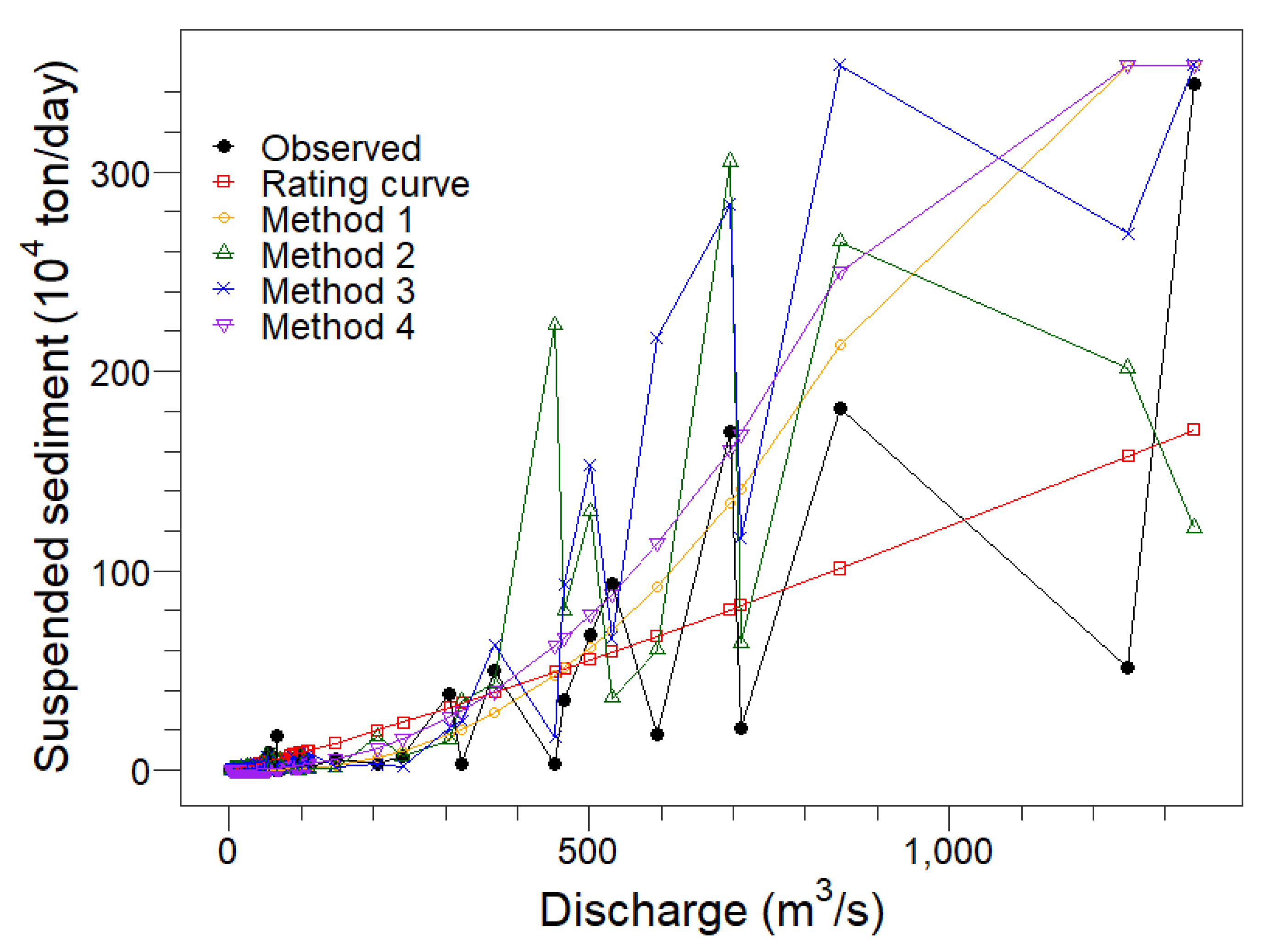
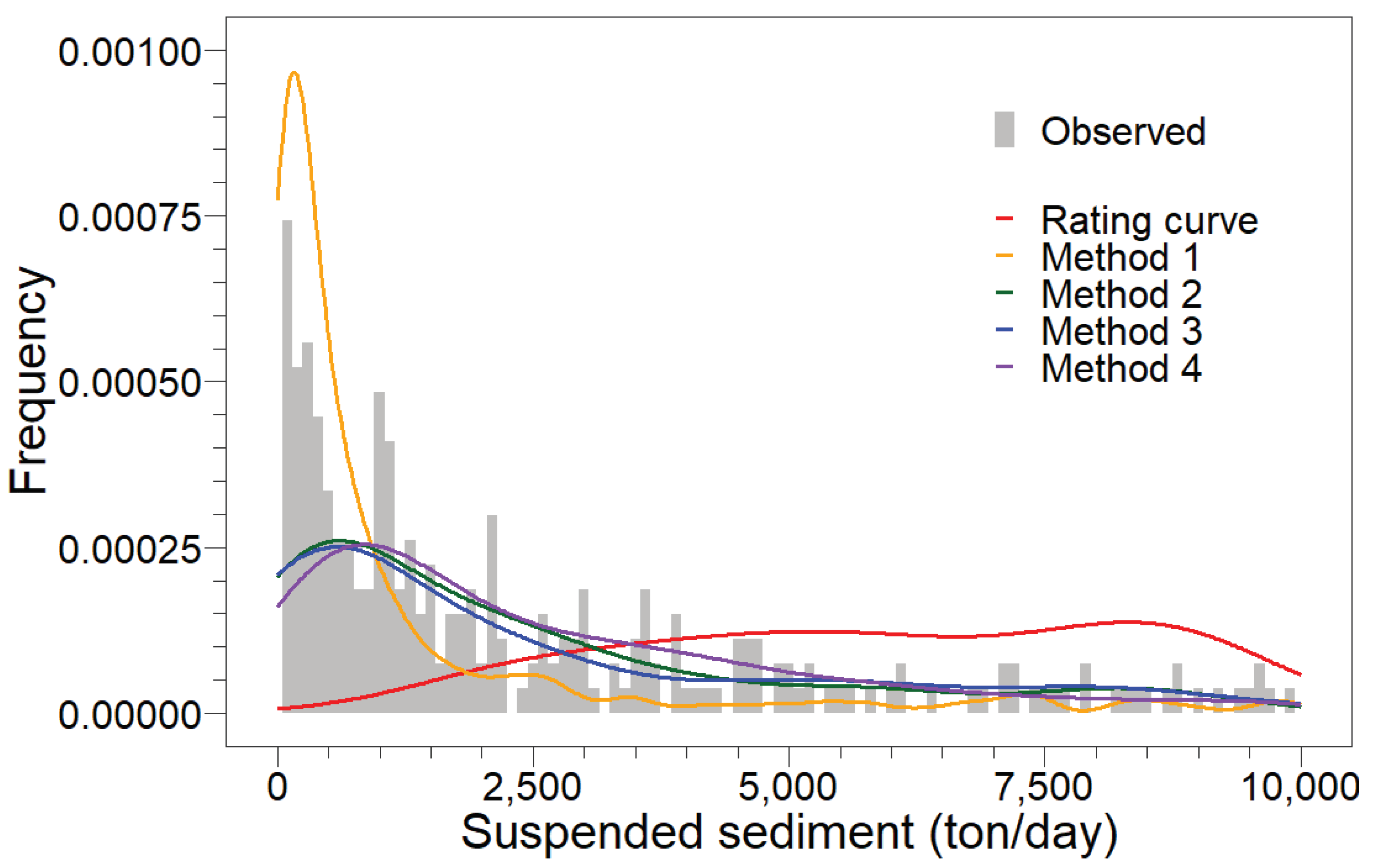
  • Method 1. The most natural thought to obtain the imputed data is the mode of the CPDF, which represents the most likely value (i.e., the quantile with the highest CPDF value).
l e = f L | q o 1 ( ψ )
where le denotes the estimated imputed sediment data with the highest CPDF value (i.e., the mode of the CPDF); and ψ denotes the maximum value of the CPDF.
  • Method 2. Di Lascio et al. [5] proposed the Hit or Miss Monte Carlo method to estimate missing data, which uses the CPDF and random numbers. The following steps are used to estimate the imputed sediment data.
Step 1. Obtain F Q ( q o ) = v by an observed discharge qo.
Step 2. From the CPDF f L | q o ( l ) in Equation (4), define the lmin and lmax as the minimum and maximum sediment loads of the CPDF, and ψ as the maximum value of the CPDF.
Step 3. Generate two random numbers r1 and r2 from the uniform distribution U(0, 1).
Step 4. Calculate e = lmin + r1(lmaxlmin).
Step 5. If r 2 ψ     f L ( e ) c ( F L ( e ) ,   v ) then le = e, else return to Step 3.
  • Method 3. Peng et al. [52] used the CCDF and a random number to infill the missing sediment data.
Step 1. Obtain F Q ( q o ) = v by an observed discharge qo.
Step 2. Generate a random number r from the uniform distribution U(0, 1).
Step 3. According to the CCDF defined in Equation (5), solve r   = C L | q o ( F L ( l ) | v ) and obtain F L ( l ) = u .
Step 4. The estimated imputed sediment load is l e = F L 1 ( u ) .
  • Method 4. Bezak et al. [18] used a similar procedure in Method 3, but with 10,000 generations, to have 10,000 imputed values, and selected the median of these 10,000 data as the imputed sediment data.

3. Data Used

3.1. Suspended Sediment Load and Streamflow Discharge Data

The recorded daily suspended sediment load and streamflow discharge data at Jenshou station (121.50° E, 23.96° N) located in the Hualian River of eastern Taiwan for the period of 1960–2019 are employed to demonstrate the proposed approach. Annual mean rainfall in the Hualian River basin is 2550 mm and approximate 70% of annual rainfall is clustered within the wet-season (June−November). Annual average temperature in this basin is 22.8 °C with highest temperatures exceeding 30 °C occurring in summer. Suspended sediment load and streamflow discharge data have been measured and collected by the Water Resource Agency in Taiwan. Basic information, including river, catchment area, data length, number of sediment and discharge data, are summarized in Table 2. Infrequent sampling of daily sediment data leading to the number of recorded suspended sediment load is approximately 2% of recorded discharge data at Jenshou station. Mean and standard deviation of entire daily discharge series and paired sediment-discharge data in the period of 1960–2019 are also reported in Table 2, respectively.
Recorded paired sediment-discharge data at Jenshou station are shown in Figure 1. Positive correlated sediment-discharge relationship is observed in Figure 1. However, clear scatter between recorded sediment and discharge data cannot be ignored, especially at the moderate- to high-flow conditions. Recorded suspended sediment load data are highly clustered below mean discharge of recorded paired data. For example, approximately 76% of sediment data are measured below 99.96 m3/s, the mean discharge of recorded paired data.
Recorded paired sediment-discharge data of the period of 1960–2019 at Jenshou station are split into two periods. Approximately 70% of recorded data of the period of 1960–2000 are employed to construct models and calibrate model parameters and the remaining data of the period of 2001–2019 are used to validate the performance of the constructed models.

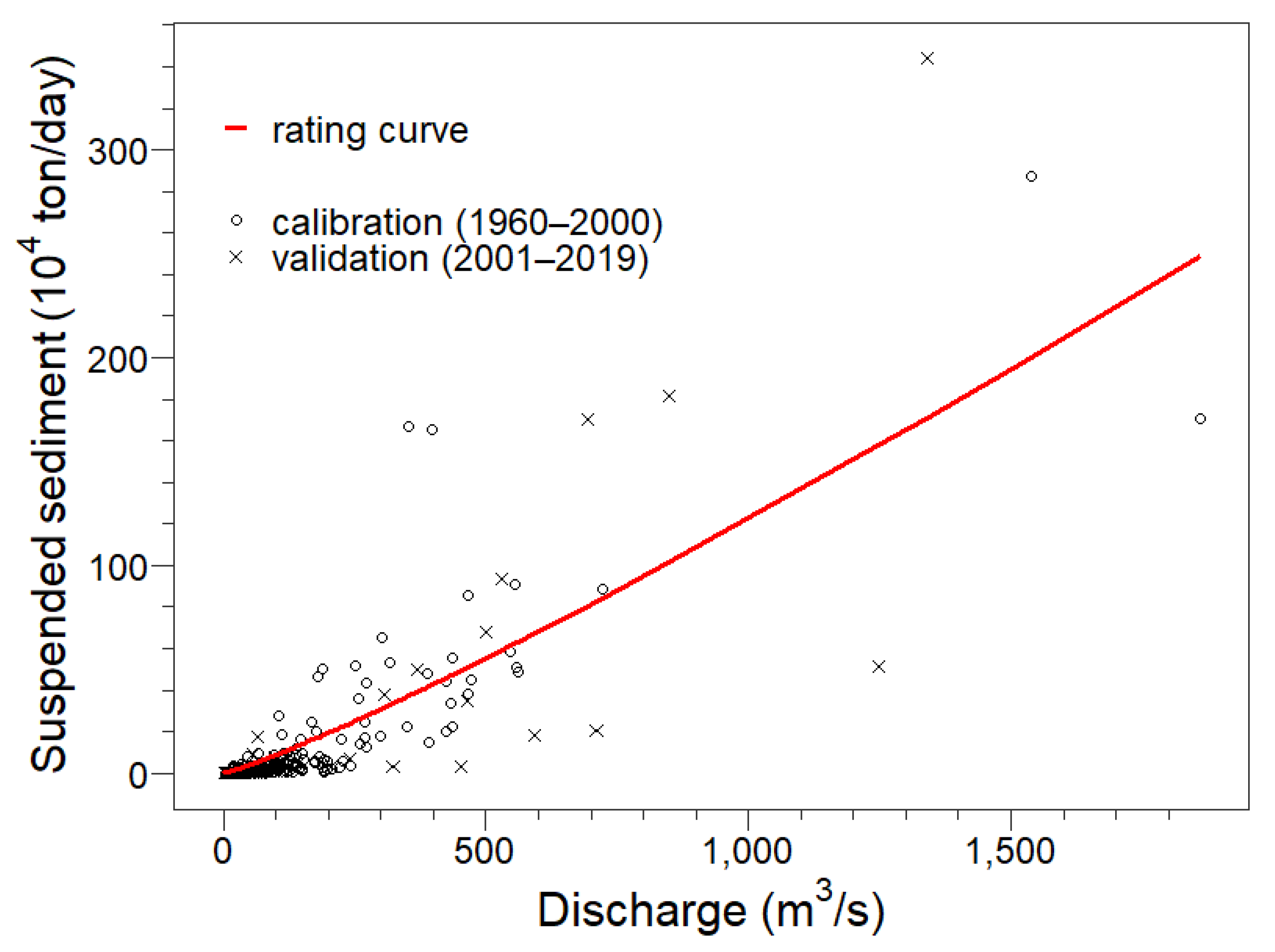
3.2. Empirical Sediment Rating Curve

The sediment rating curve is a traditional approach to infilling sediment data based on the empirical relationship between recorded sediment and discharge data. A commonly used relationship between sediment and discharge data is the power law function, which is expressed as
L = a Q b
where L and Q denote suspended sediment load and streamflow discharge, respectively; and a and b are coefficients which are estimated from recorded data.
The empirical sediment rating curve at Jenshou station, shown in Figure 1, is determined by nonlinear least squares regression [58] based on recorded data of the period of 1960–2000. The empirical sediment rating curve at Jenshou station is written as
L ^ = 448.82 Q 1.1449
where L ^ denotes the estimated suspended sediment load in unit of ton/day; and Q is recorded streamflow discharge in unit of m3/s.

4. Results and Discussion

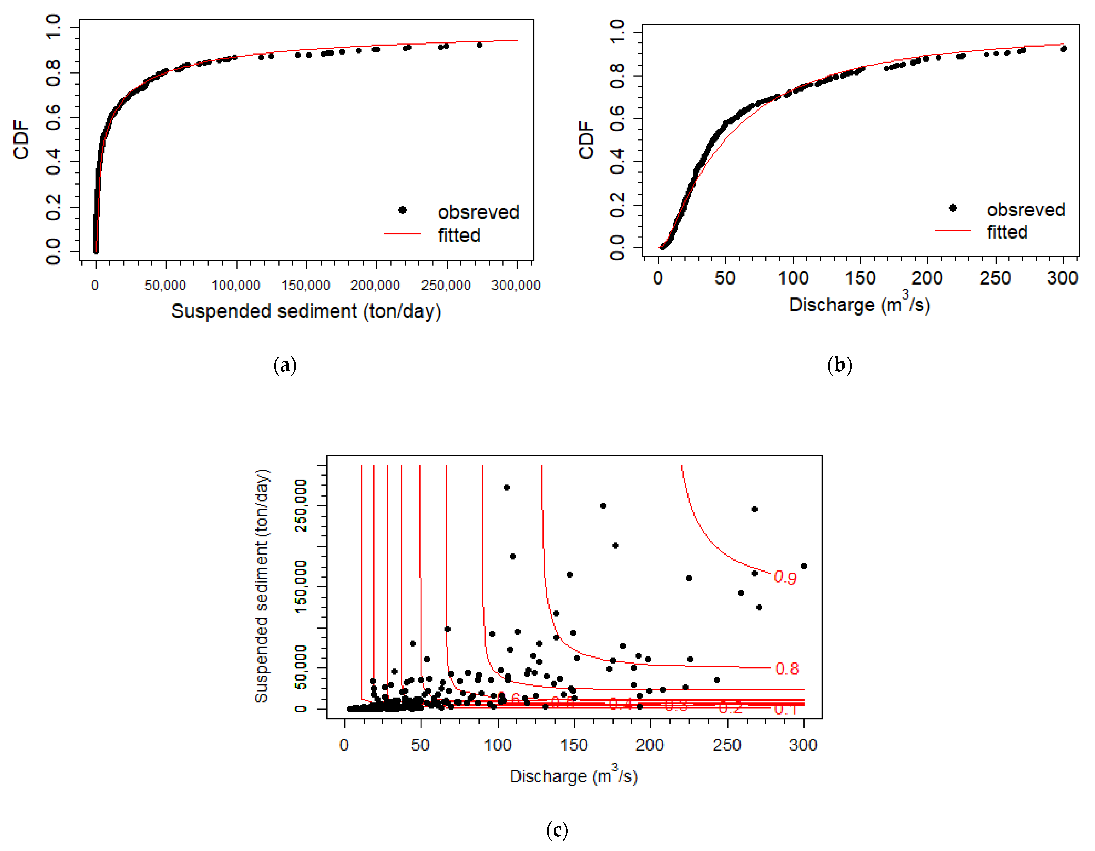
4.1. The Best-Fitted Marginal Distributions and Copulas

A total of five widely used two-parameter distributions, including normal (NO), lognormal (LNO), gamma (GA), Gumbel (GU), and Weibull (WEI), are used to model the suspended sediment load and streamflow discharge. Distribution parameters are estimated by the maximum likelihood method. The goodness-of-fit of each distribution for sediment load and discharge are accessed by the K-S test and the best-fitted distribution is determined by the minimum AIC. The recorded daily suspended sediment load and discharge at Jenshou station for the period of 1960–2000 are best-fitted by the lognormal distribution with the corresponding parameters are summarized in Table 3. The PDFs of suspended sediment load and discharge are respectively written as
f L ( l ) = 1 2 π l × 2.456 exp [ ( ln l 8.753 ) 2 2 × 2.456 2 ]
f Q ( q ) = 1 2 π q × 1.134 exp [ ( ln q 3.898 ) 2 2 × 1.134 2 ]
Figure 2a,b illustrates the fitted lognormal distributions associated with recorded suspended sediment and discharge, respectively. Good agreements between the fitted distribution and recorded data for sediment and discharge are observed in Figure 2.
The IFM is used to estimate copula parameter, the C-M test is then used to access goodness-of-fit of each copula, and the minimum AIC is employed to determine the best-fitted copula. The best-fitted copula for the paired sediment-discharge data (period of 1960–2000) at Jenshou station is the Gumbel-Hougaard copula. The copula parameter is also reported in Table 3. Copula-based JCDF of sediment and discharge is written as
F L Q ( l ,   q ) = C ( F L ( l ) ,   F Q ( q ) ) = exp { [ ( ln F L ( l ) ) 2.97 + ( ln F Q ( q ) ) 2.97 ] 1 2.97 }
where FL(l) and FQ(q) denote the values of CDFs of suspended sediment load and discharge, respectively, which are determined by
F L ( l ) = 0 l 1 2 π l × 2.456 exp [ ( ln l 8.753 ) 2 2 × 2.456 2 ] d l
F Q ( q ) = 0 q 1 2 π q × 1.134 exp [ ( ln q 3.898 ) 2 2 × 1.134 2 ] d q
Figure 2c illustrates the contours of probabilities determined by the fitted copula associated with recorded paired sediment-discharge data.

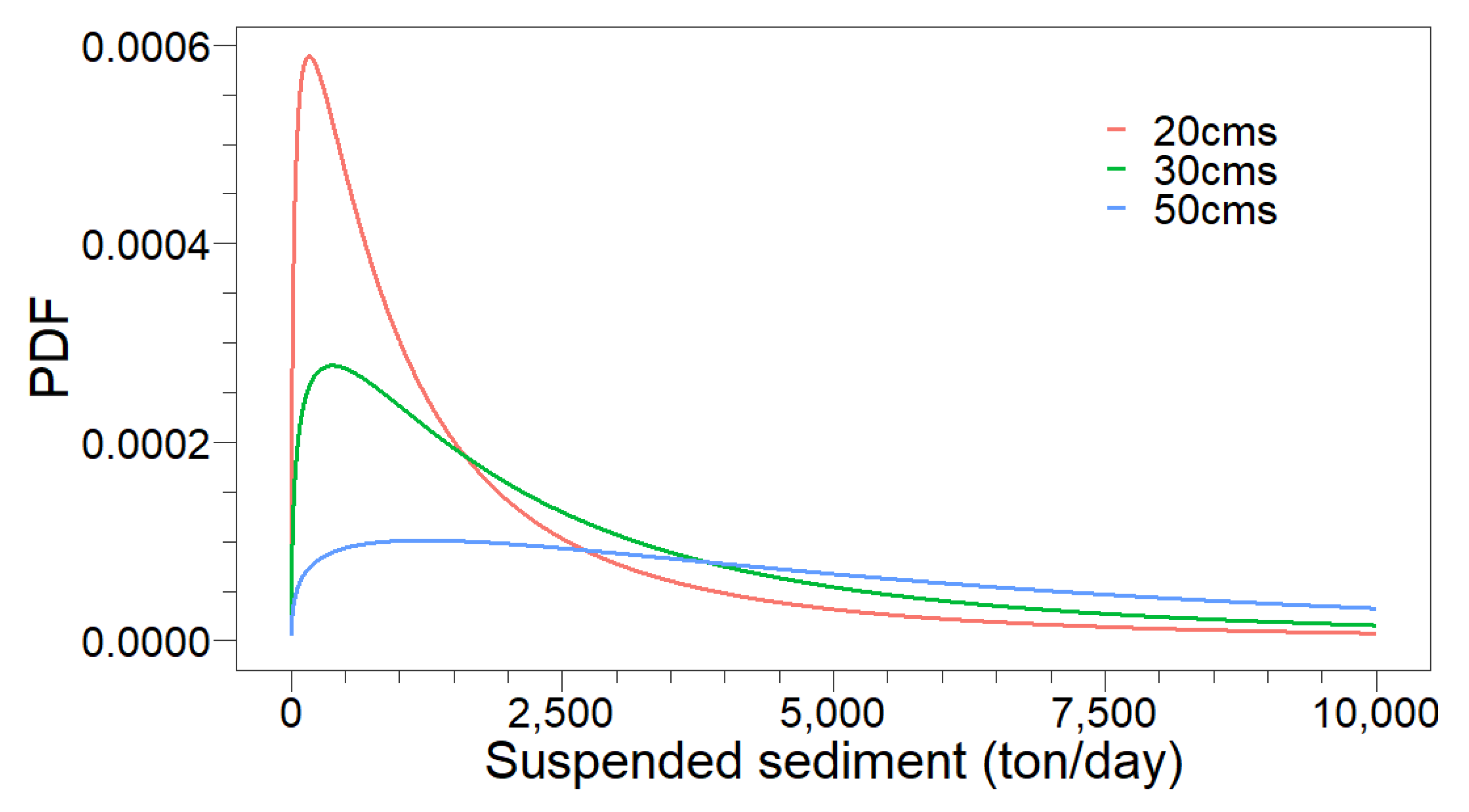
4.2. Probabilistic Sediment Estimations Using Copula-Based Conditional Probability Density Function

Probabilistic estimation of missing suspended sediment load is made possible using the copula-based CPDF and CCDF of sediment given an observed discharge q o (Equations (4) and (5)) and the best-fitted distributions of sediment and discharge (Equations (9)–(13)). The copula-based CPDF and CCDF of sediment given observed discharge at Jenshou station are given below, respectively.
f L | q o ( l ) = 1 6.156 × l e ( ln l 8.753 ) 2 12.064 e [ ( ln F L ( l ) ) 2.97 + ( ln F Q ( q o ) ) 2.97 ] 1 2.97 [ ( ln F L ( l ) ) ( ln F Q ( q o ) ) ] 1.97 F L ( l ) F Q ( q o ) [ ( ln F L ( l ) ) 2.97 + ( ln F Q ( q o ) ) 2.97 ] 1.327 { 1.97 × [ ( ln F L ( l ) ) 2.97 + ( ln F Q ( q o ) ) 2.97 ] 1 2.97 + 1 }
F L | q o ( l ) = e [ ( ln F L ( l ) ) 2.97 + ( ln F Q ( q o ) ) 2.97 ] 1 2.97 [ 1 + ( ln F L ( l ) ln F Q ( q o ) ) 2.97 ] 1 2.97 1 1 F Q ( q o )
where q o denotes an observed discharge.
Figure 3 illustrates the CPDFs of suspended sediment load given observed discharge equals 20, 30, and 50 m3/s for demonstration. The derived CPDFs quantify the estimation uncertainty of suspended sediment load. For example, given the observed discharge of 20 m3/s, the probabilities that suspended sediment loads exceeding 100, 1000, and 5000 ton/day are 0.955, 0.547, and 0.133, respectively. Given the observed discharge of 30 m3/s, the interquartile range of suspended sediment load is bounded between 989 and 5348 ton/day. The probability that the suspended sediment load ranged between 1000 and 5000 ton/day is 0.349 given the observed discharge of 50 m3/s.
The CPDFs generally shift rightward and become flat with increasing discharge. For instance, the modes of the CPDFs given a discharge of 20, 30, and 50 m3/s are 168, 384, and 1226 ton/day, respectively. The flat CPDF of a greater discharge implies that suspended sediment load is distributed in a very large range. That is, greater uncertainties exist in an estimation of suspended sediment load for the condition of large discharge. For instance, the interquartile range increases from 2327 ton/day for the observed discharge of 20 m3/s to 4359 and 10,087 ton/day for observed discharges of 30 and 50 m3/s, respectively.
The inherently scattered relationship between recorded sediment and discharge leads to different recorded sediments observed for nearly identical discharge. For instance, recorded suspended sediment loads of 1250.4, 3944.3, 2084.0, 960.3, and 1379.0 ton/day are noted for discharges of 19.8, 20.1, 20.1, 20.0, and 19.8 m3/s, respectively. The scattered characteristics are captured by the derived CPDF shown in Figure 3, which provides probabilistic estimation of missing sediment data. However, single-value estimation of sediment data is often required in practical applications.

4.3. Single-Value Sediment Estimations

Four different methods based on the derived copula-based CPDF and CCDF associated with sediment rating curve are used to estimate the suspended sediment loads given the observed discharge for the period of 2001–2019 in this study. The estimations of these methods are compared with recorded data, shown in Figure 4, and evaluated in terms of root mean square error (RMSE), mean absolute percentage error (MAPE), Nash-Sutcliffe efficiency (NSE) [59], and modified Nash-Sutcliffe efficiency (MNSE) [60], which are defined below, respectively.
RMSE = 1 n i = 1 n ( l ^ i l i ) 2
MAPE = 100 n i = 1 n | l ^ i l i l i |
NSE = 1 i = 1 n ( l ^ i l i ) 2 i = 1 n ( l ^ i l ¯ ) 2
MNSE = 1 i = 1 n | l ^ i l i | i = 1 n | l ^ i l ¯ |
where n denotes the number of data; l i and l ^ i denote the ith observed and estimated sediment data, respectively; and l ¯ denotes the mean observed sediment.
The model with smaller RMSE and MAPE and close-to-1 NSE and MNSE denotes that it has better capability to infill missing data and has fewer deviations from the observed data. The results of RMSE, MAPE, NSE, and MNSE of these five infilling methods for the calibration (1960–2000) and validation (2001–2019) periods are reported in Table 4. The results indicate that sediment rating curve has best performance in RMSE and NSE. On the other hand, copula-based models (Methods 1–4) generally outperform in MAPE and MNSE and Method 1 (infilling missing value by mode) is the best model. Sediment rating curve is obtained by the least squares regression with minimized least squared deviations from the recorded data. It thus leads to better performance in criteria with the square term such as RMSE and NSE. Conditional distribution-based infilling methods, on the other hand, outperform in the other criteria.

4.4. Discussion

Different evaluations on these sediment estimations are explored in this section. The estimated sediment of the periods of 1960–2000 (calibration), 2001–2019 (validation), and 1960–2019 are categorized as low, moderate, and high flows with 30, 40 and 30% of data in each flow state. Evaluations in terms of RMSE, MAPE, NSE, and MNSE of these sediment estimations for various periods are summarized in Table 5. Similar performances of these estimation methods are observed for various periods. Sediment rating curve loses its dominance in all indices for the low- and moderate-flow states. In contrast, Method 4 (median of 10,000 sediment estimations based on CCDF) outperforms other methods in several indices for these two flow states. However, sediment rating curve is the best model in RMSE and NSE and Method 1 outperforms in MAPE and MNSE of high-flow state for various periods.
Different performance evaluations between Table 4 and Table 5 are attributed to different infilling schemes used in various methods. The worse performances of sediment rating curve in low- and moderate-flow states are caused by its overestimations of sediment. The overestimations in low- and moderate-flow states do not produce greater squared deviations from the recorded data due to smaller sediment loads in low- and moderate-flow states. Fewer deviations in high-flow states lead to the sediment rating curve with better performance in RMSE and NSE of high-flow states for various periods (Table 5).
Methods 1 to 4 depend on the derived conditional distributions to estimate the sediments in all flow states. No clear overestimations for these conditional distribution-based methods are observed in low- and moderate-flow states (Figure 3) and induce better performance for all indices. However, less squared deviations for the sediment rating curve observed in high-flow state lead to only Method 1 (infilling missing value by mode) outperforming in MAPE and MNSE.
Figure 5 illustrates the frequency histograms of observed sediment data and the estimations of various infilling methods for the period of 1960–2019. The results indicate that the sediment rating curve produces a histogram contradicting the histogram of the observed sediment data. This contradiction is induced by overestimations for smaller sediments, which are evidently observed for the low-flow state in Figure 4 and Table 5. In contrast, copula-based Methods 1–4 generate high frequencies in smaller sediments and low frequencies in greater sediments. However, similar histograms among Methods 2–4 are close to the histogram of recorded sediments when sediments exceed 1000 ton/day. Only Method 1 (infilling missing value by mode) reflects the similarity in all scopes of suspended sediment load. This similarity between histograms of recorded sediments and the estimated sediments by Method 1, especially when sediment <1000 ton/day, is attributed to the right-skewed CPDFs shown in Figure 3. Method 1 estimates sediments using the mode of the CPDFs, which is clustered in smaller sediments due to right-skewed CPDFs and leads to high frequencies in smaller sediments.
Shojaeezadeh et al. [9] and Guo et al. [50] indicated that greater discharges are associated with larger intervals of conditional marginal distribution of sediments. Further, the relationship between discharge and sediment is nonlinear and highly stochastic. That is, a similar discharge can yield hugely different sediments. These properties of probabilistic sediment estimations are in line with the results of copula-based CPDFs shown in Figure 3. Bezak et al. [18] revealed that a copula-based estimation model yields the worst fit (greatest RMSE) when compared with the results of multiple regression and exponential models in some cases. However, a copula-based model produces the smallest residuals and better results in low-medium-flow events. These findings are consistent with the results of this study reported in Table 5.

5. Conclusions

Based on the daily paired sediment-discharge data at Jenshou station located in eastern Taiwan for the period of 1960–2019, probabilistic and four single-value estimation models of sediment data are constructed using copulas. The Gumbel-Hougaard copula (Figure 2c) is used to model the joint probability distribution of discharge and sediment data with best-fitted lognormal distributions (Figure 2a,b) as the marginal distributions.
The copula-based CPDF (Figure 3) and CCDF of sediments given various observed discharges provide probabilistic properties of estimated sediments such as the highly likely range of estimations, probabilities of sediments greater than or less than certain values, and various quantiles of specific probabilities. The derived CPDFs at Jenshou station shift toward the right and become flatter with increasing discharge. This phenomenon implies that the estimated suspended sediment load is distributed in a very large range for a greater discharge. That is, greater uncertainties exist in an estimation of suspended sediment load for the condition of large discharge.
The results of single-value sediment estimations for various infilling methods indicate that no single method outperforms in all evaluation criteria. The sediment rating curve has the best performance in RMSE and NSE, while copula-based methods generally outperform in MAPE and MNSE and Method 1 (infilling missing value by mode) is the best model among these copula-based methods. However, the frequency histogram of infilled sediments by the sediment rating curve contradicts the frequency histogram of recorded sediment. In contrast, the infilled sediments of the copula-based methods preserve a similar frequency histogram as noted in the recorded sediments. That is, high frequency is observed in small sediment and low frequency occurs in great sediment. Among these four methods, the frequency histogram of Method 1 is close to that of recorded sediment data.
Infilling missing sediments to have long and continuous data provides the necessary information for design and operation of water-resources engineering. Statistical methods alleviate the need for physical factors of watersheds and rivers to infill sediments. However, uncertainties existing in estimated sediments are attributed to the proposed statistical models using discharge only. Incorporating additional available parameters such as rainfall and maintaining models to increase the accuracy of infilled sediments remain as topics for further extending this study. Additionally, selecting the best estimation method among the conflicting indices using the multi-criteria evaluation approach is also important in model construction processes.

Author Contributions

Conceptualization, J.-T.S.; methodology, J.-T.S.; software, Y.-C.L.; formal analysis, J.-T.S., and Y.-C.L.; data curation, Y.-C.L.; writing—original draft preparation, J.-T.S.; writing—review and editing, J.-T.S.; funding acquisition, J.-T.S. All authors have read and agreed to the published version of the manuscript.

Funding

This research was funded by Ministry of Science and Technology, Taiwan, ROC, grant number MOST 108-2221-E-006-016.

Institutional Review Board Statement

Not applicable.

Informed Consent Statement

Not applicable.

Data Availability Statement

The suspended sediment load and streamflow data used in this study are provided from Water Resources Agency, Taiwan (https://www.wra.gov.tw (accessed on 18 June 2021)).

Acknowledgments

Financial support for this study was graciously provided by the Ministry of Science and Technology, Taiwan, ROC (MOST 108-2221-E-006-016). Valuable comments from three anonymous referees for improving presentation are greatly appreciated.

Conflicts of Interest

The authors declare no conflict of interest.

References

  1. Bárdossy, A.; Pegram, G. Infilling missing precipitation records—A comparison of a new copula-based method with other techniques. J. Hydrol. 2014, 519, 1162–1170. [Google Scholar] [CrossRef]
  2. Kalteh, A.M.; Hjorth, P. Imputation of missing values in a precipitation—runoff process database. Hydrol. Res. 2009, 40, 420–432. [Google Scholar] [CrossRef]
  3. Ben Aissia, M.A.; Chebana, F.; Ouarda, T.B.M.J. Multivariate missing data in hydrology—Review and applications. Adv. Water Resour. 2017, 110, 299–309. [Google Scholar] [CrossRef] [Green Version]
  4. Käärik, E.; Käärik, M. Modeling dropouts by conditional distribution, a copula-based approach. J. Stat. Plan. Inference 2009, 139, 3830–3835. [Google Scholar] [CrossRef]
  5. Di Lascio, F.M.L.; Giannerini, S.; Reale, A. Exploring copulas for the imputation of complex dependent data. Stat. Methods Appl. 2015, 24, 159–175. [Google Scholar] [CrossRef]
  6. Hamzah, F.B.; MohdHamzah, F.; Razali, S.F.M.; Jaafar, O.; AbdulJamil, N. Imputation methods for recovering streamflow observation: A methodological review. Cogent Environ. Sci. 2020, 6, 1745133. [Google Scholar] [CrossRef]
  7. Yang, C.T. Sediment Transport Theory and Practice; McGraw-Hill: New York, NY, USA, 1996. [Google Scholar]
  8. Walling, D.E. Human impact on land-ocean sediment transfer by the world’s rivers. Geomorphology 2006, 79, 192–216. [Google Scholar] [CrossRef]
  9. Shojaeezadeh, S.A.; Nikoo, M.R.; McNamara, J.; AghaKouchak, A.; Sadegh, M. Stochastic modeling of suspended sediment load in alluvial rivers. Adv. Water Resour. 2018, 119, 188–196. [Google Scholar] [CrossRef]
  10. Walling, D.E. Assessing the accuracy of suspended sediment rating curves for a small basin. Water Resour. Res. 1977, 13, 531–538. [Google Scholar] [CrossRef]
  11. Jain, S.K. Development of integrated sediment rating curves using ANNs. J. Hydraul. Eng. 2001, 127, 30–37. [Google Scholar] [CrossRef]
  12. Kişi, Ö. Suspended sediment estimation using neuro-fuzzy and neural network approaches. Hydrol. Sci. J. 2005, 50, 683–696. [Google Scholar] [CrossRef]
  13. Çimen, M. Estimation of daily suspended sediments using support vector machines. Hydrol. Sci. J. 2008, 53, 656–666. [Google Scholar] [CrossRef]
  14. Vigiak, O.; Bende-Michl, U. Estimating bootstrap and Bayesian prediction intervals for constituent load rating curve. Water Resour. Res. 2013, 49. [Google Scholar] [CrossRef] [Green Version]
  15. Kitsikoudis, V.; Sidiropoulos, E.; Hrissanthou, V. Machine learning utilization for bed load transport in gravel-bed rivers. Water Resour. Manag. 2014, 28, 3727–3743. [Google Scholar] [CrossRef]
  16. Shiau, J.T.; Chen, T.J. Quantile regression-based probabilistic estimation scheme for daily and annual suspended sediment loads. Water Resour. Manag. 2015, 29, 2805–2818. [Google Scholar] [CrossRef]
  17. Kisi, O.; Zounemat-Kermani, M. Suspended sediment modeling using neuro-fuzzy embedded fuzzy c-means clustering techniques. Water Resour. Manag. 2016, 30, 3979–3994. [Google Scholar] [CrossRef]
  18. Bezak, N.; Rusjan, S.; Fijavž, M.K.; Mikoš, M.; Šraj, M. Estimation of suspended sediment loads using copula functions. Water 2017, 9, 628. [Google Scholar] [CrossRef] [Green Version]
  19. Mirakhorlo, M.S.; Rahimzadegan, M. Application of sediment rating curves to evaluate efficiency of EPM and MPSIAC using RS and GIS. Environ. Earth Sci. 2018, 77, 723. [Google Scholar] [CrossRef]
  20. Al-Mukhtar, M. Random forest, support vector machine, and neural networks to modelling suspended sediment in Tigris River-Baghdad. Environ. Monit. Assess. 2019, 191, 673. [Google Scholar] [CrossRef]
  21. Tao, H.; Keshtegar, B.; Yaseen, Z.M. The feasibility of integrative radial basis M5Tree predictive model for river suspended sediment load simulation. Water Resour. Manag. 2019, 33, 4471–4490. [Google Scholar] [CrossRef]
  22. Salih, S.Q.; Sharafati, A.; Khosravi, K.; Faris, H.; Kisi, O.; Tao, H.; Ali, M.; Yaseen, Z.M. River suspended sediment load prediction based on river discharge information: Application of newly developed data mining models. Hydrol. Sci. J. 2020, 65, 624–637. [Google Scholar] [CrossRef]
  23. Hazarika, B.B.; Gupta, D.; Berlin, M. Modeling suspended sediment load in a river using extreme learning machine and twin support vector regression with wavelet conjunction. Environ. Earth Sci. 2020, 79, 234. [Google Scholar] [CrossRef]
  24. Sharafati, A.; Asadollah, S.B.H.S.; Motta, D.; Yaseen, Z.M. Application of newly developed ensemble machine learning models for daily suspended sediment load prediction and related uncertainty analysis. Hydrol. Sci. J. 2020, 65, 2022–2042. [Google Scholar] [CrossRef]
  25. Yadav, A.; Chatterjee, S.; Equeenuddin, S.M. Suspended sediment yield modeling in Mahanadi River, India by multi-objective optimization hybridizing artificial intelligence algorithm. Int. J. Sediment Res. 2021, 36, 76–91. [Google Scholar] [CrossRef]
  26. Idrees, M.B.; Jehanzaib, M.; Kim, D.; Kim, T.W. Comprehensive evaluation of machine learning models for suspended sediment load inflow prediction in a reservoir. Stoch. Environ. Res. Risk Assess. 2021. [Google Scholar] [CrossRef]
  27. Gupta, D.; Hazarika, B.B.; Berlin, M.; Sharma, U.M.; Mishra, K. Artificial intelligence for suspended sediment load prediction: A review. Environ. Earth Sci. 2021, 80, 346. [Google Scholar] [CrossRef]
  28. Kao, S.C.; Govindaraju, R.S. A copula-based joint deficit index for droughts. J. Hydrol. 2010, 380, 121–134. [Google Scholar] [CrossRef]
  29. Lee, T.; Salas, J.D. Copula-based stochastic simulation of hydrological data applied to Nile River flows. Hydrol. Res. 2011, 42, 318–330. [Google Scholar] [CrossRef]
  30. Reddy, M.J.; Ganguli, P. Application of copulas for derivation of drought severity-duration-frequency curves. Hydrol. Process. 2012, 26, 1672–1685. [Google Scholar] [CrossRef]
  31. Shiau, J.T.; Hsiao, Y.Y. Water-deficit-based drought risk assessment in Taiwan. Nat. Hazards 2012, 64, 237–257. [Google Scholar] [CrossRef]
  32. Chebana, F.; Ouarda, T.B.M.J.; Duong, T.C. Testing for multivariate trends in hydrologic frequency analysis. J. Hydrol. 2013, 486, 519–530. [Google Scholar] [CrossRef]
  33. Callau Ponduje, A.C.; Belli, A.; Haberlandt, U. Dam risk assessment based on univariate versus bivariate statistical approaches: A case study for Argentina. Hydrol. Sci. J. 2014, 59, 2216–2232. [Google Scholar] [CrossRef] [Green Version]
  34. Masina, M.; Lamberti, A.; Archetti, R. Coastal flooding: A copula based approach for estimating the joint probability of water levels and waves. Coast. Eng. 2015, 97, 37–52. [Google Scholar] [CrossRef]
  35. Requena, A.I.; Flores, I.; Mediero, L.; Garrote, L. Extension of observed flood series by combining a distributed hydro-meteorological model and a copula-based model. Stoch. Environ. Res. Risk Assess. 2016, 30, 1363–1378. [Google Scholar] [CrossRef] [Green Version]
  36. Dodangeh, E.; Shahedi, K.; Shiau, J.T.; Mirakbari, M. Spatial hydrological drought characteristics in Karkheh River basin, southwest Iran using copulas. J. Earth Syst. Sci. 2017, 126, 80. [Google Scholar] [CrossRef]
  37. Qian, L.; Wang, H.; Dang, S.; Wang, C.; Jiao, Z.; Zhao, Y. Modelling bivariate extreme precipitation distribution for data-scare regions using Gumbel-Hougaard copula with maximum entropy estimation. Hydrol. Process. 2018, 32, 212–227. [Google Scholar] [CrossRef]
  38. Mazdiyasni, O.; Sadegh, M.; Chiang, F.; AghaKouchak, A. Heat wave intensity duration frequency curve: A multivariate approach for hazard and attribution analysis. Sci. Rep. 2019, 9, 14117. [Google Scholar] [CrossRef] [PubMed]
  39. Dondangeh, E.; Shahedi, K.; Solaimani, K.; Shiau, J.T.; Abraham, J. Data-based bivariate uncertainty assessment of extreme rainfall-runoff using copulas: Comparison between annual maximum series (AMS) and peaks over threshold (POT). Environ. Monit. Assess. 2019, 191, 67. [Google Scholar] [CrossRef]
  40. Ben Nasr, I.; Chebana, F. Homogeneity testing of multivariate hydrological records, using multivariate copula L-moments. Adv. Water Resour. 2019, 134, 103449. [Google Scholar] [CrossRef]
  41. Bushra, N.; Trepanier, J.C.; Rohli, R.C. Joint probability risk modeling of storm surge and cyclone wind along the coast of Bay of Bengal using a statistical copula. Int. J. Climatol. 2019, 39, 4206–4217. [Google Scholar] [CrossRef]
  42. Tahroudi, M.N.; Ramezani, Y.; De Michele, C.; Mirabbasi, R. Analyzing the conditional behavior of rainfall deficiency and groundwater level deficiency signatures by using copula functions. Hydrol. Res. 2020, 51, 1332–1348. [Google Scholar] [CrossRef]
  43. Botai, C.M.; Botai, J.O.; Adeola, A.M.; de Wit, J.P.; Ncongwane, K.P.; Zwane, N.N. Drought risk analysis in the Eastern Cape Province of South Africa: The copula lens. Water 2020, 12, 1938. [Google Scholar] [CrossRef]
  44. Singh, H.; Pirani, F.J.; Najafi, M.R. Characterizing the temperature and precipitation covariability over Canada. Theor. Appl. Climatol. 2020, 139, 1543–1558. [Google Scholar] [CrossRef]
  45. Uttarwar, S.B.; Barma, S.D.; Mahesha, A. Bivariate modeling of hydroclimatic variables in humid tropical coastal region using Archimedean copulas. J. Hydrol. Eng. 2020, 25, 05020026. [Google Scholar] [CrossRef]
  46. Zhong, M.; Zeng, T.; Jiang, T.; Wu, H.; Chen, X.H.; Hong, Y. A copula-based multivariate probability analysis for flash flood risk under the compound effect of soil moisture and rainfall. Water Resour. Manag. 2021, 35, 83–98. [Google Scholar] [CrossRef]
  47. Sajeev, A.; Barma, D.; Mahesha, A.; Shiau, J.T. Bivariate drought characterization of two contrasting climatic regions in India using copula. J. Irrig. Drain. Eng. 2021, 147, 05020005. [Google Scholar] [CrossRef]
  48. Zhang, J.; Ding, Z.; You, J. The joint probability distribution of runoff and sediment and its change characteristics with multi-time scales. J. Hydrol. Hydromech. 2014, 62, 218–225. [Google Scholar] [CrossRef] [Green Version]
  49. Bezak, N.; Mikoš, M.; Šraj, M. Trivariate frequency analyses of peak discharge, hydrograph volume and suspended sediment concentration data using copulas. Water Resour. Manag. 2014, 28, 2195–2212. [Google Scholar] [CrossRef]
  50. Guo, A.; Chang, J.; Wang, Y.; Huang, Q. Variations in the runoff-sediment relationship of the Weihe River basin based on the copula function. Water 2016, 8, 223. [Google Scholar] [CrossRef] [Green Version]
  51. Huang, S.; Li, P.; Huang, Q.; Leng, G. Copula-based identification of the non-stationarity of the relation between runoff and sediment load. Int. J. Sediment Res. 2017, 32, 221–230. [Google Scholar] [CrossRef]
  52. Peng, Y.; Yu, X.; Yan, H.; Zhang, J. Stochastic simulation of daily suspended sediment concentration using multivariate copulas. Water Resour. Manag. 2020, 34, 3913–3932. [Google Scholar] [CrossRef]
  53. Peng, Y.; Shi, Y.; Yan, H.; Zhang, J. Multivariate frequency analysis of annual maxima suspended sediment concentrations and floods in the Jinsha River China. J. Hydrol. Eng. 2020, 25, 05020029. [Google Scholar] [CrossRef]
  54. Sklar, K. Fonctions de repartition à n dimensions et leura marges. Publ. Inst. Stat. Univ. Paris 1959, 8, 229–231. [Google Scholar]
  55. Joe, H. Multivariate Models and Dependence Concepts; Chapman and Hall: New York, NY, USA, 1997. [Google Scholar]
  56. Nelsen, R.B. An Introduction to Copulas; Springer: New York, NY, USA, 1999. [Google Scholar]
  57. Genest, C.; Remillard, B.; Beaudoin, D. Goodness-of-fit tests for copulas: A review and a power study. Insur. Math. Econ. 2009, 44, 199–213. [Google Scholar] [CrossRef]
  58. Asselman, N.E.M. Fitting and interpretation of sediment rating curve. J. Hydrol. 2000, 234, 228–248. [Google Scholar] [CrossRef]
  59. Nash, J.E.; Sutcliffe, J.V. River flow forecasting through conceptual model part I—A discussion of principle. J. Hydrol. 1970, 10, 282–290. [Google Scholar] [CrossRef]
  60. Legates, D.R.; McCabe, G.J., Jr. Evaluating the use of goodness-of-fit measures in hydrologic and hydroclimatic model validation. Water Resour. Res. 1999, 35, 233–241. [Google Scholar] [CrossRef]
Figure 1. Scatter diagram of recorded daily suspended sediment load and streamflow discharge and the corresponding sediment rating curve at Jenshou station.
Water 13 01701 g001
Figure 2. (a) Fitted lognormal distribution associated with recorded suspended sediment load, (b) fitted lognormal distribution associated with recorded discharge, (c) contour plots of joint CDF of sediment and discharge by Gumbel-Hougaard copula and recorded paired data at Janshou station for the period of 1960–2000.
Water 13 01701 g002
Figure 3. The CPDFs of suspended sediment load given observed discharge equals 20, 30, and 50 m3/s, respectively.
Water 13 01701 g003
Figure 4. Infilled suspended sediment loads of various methods associated with the recorded data for the period of 1960–2019.
Water 13 01701 g004
Figure 5. The frequency histograms of suspended sediment load of observed data associated with results of various infilling methods for the period of 1960–2019.
Water 13 01701 g005
Table 1. Summaries of copulas and the corresponding copula densities and range of parameter used in this study.
NameCopulaCopula DensityRange of Parameter
Clayton C ( u ,   v ) = ( u θ + v θ 1 ) 1 θ c ( u ,   v ) = ( θ + 1 ) ( u θ + v θ 1 ) 1 θ 2 ( u v ) θ 1 θ     0
Frank C ( u ,   v ) = 1 θ ln 1 + ( e θ u 1 ) ( e θ v 1 ) e θ 1 c ( u , v ) = θ e θ ( u + v ) ( e θ 1 ) [ e θ ( u + v ) e θ u e θ v + e θ ] 2 θ     0
Gumbel-Hougaard C ( u ,   v ) = exp { [ ( ln u ) θ + ( ln v ) θ ] 1 θ } c ( u , v ) = C ( u ,   v ) [ ( ln u ) ( ln v ) ] θ 1 u v
[ ( ln u ) θ + ( ln v ) θ ] 2 θ 2 { ( θ 1 ) [ ( ln u ) θ + ( ln v ) θ ] 1 θ + 1 }
θ     1
Table 2. Basic information of suspended sediment load and discharge data at Jenshou station in Taiwan.
StationRiverCatchment Area
(km2)
Data LengthNumber of Sediment
Data
Number of Discharge
Data
Percentage
(%)
Sediment
(104 ton/day)
Discharge
(m3/s)
MeanStd.MeanStd.
JenshouHualian425.91960–2019 21,898 21.2865.2
1960–20194274271.98.5530.999.96187.9
Table 3. The best-fitted marginal distributions and copula for suspended sediment load and discharge.
StationSediment LoadDischargeCopula
Dist.ParametersDist.ParametersDist.Parameter
JenshouLNOμ = 8.753σ = 2.456LNOμ = 3.898σ = 1.134Gumbel-Hougaardθ = 2.97
Table 4. The results of RMSE, MAPE, NSE, and MNSE for various infilling methods for calibration (1960–2000) and validation (2001–2019).
IndexCalibration (1960–2000)Validation (2001–2019)
Rating CurveMethod 1Method 2Method 3Method 4Rating CurveMethod 1Method 2Method 3Method 4
RMSE146,424.5 a182,177.6179,157.3254,951.8184,142.6226,631.6 a298,106.7268,855.1311,492.7316,581.9
MAPE3033.9119.3 a12,154.61338.9352.81365.494.8 a341.2270.0120.5
NSE0.7068 a0.54650.56110.11110.53630.6445 a0.38480.49960.32840.3062
MNSE0.50440.5856 a0.50160.42920.56400.48260.5872a0.47240.51200.5593
Note: a denotes the best result.
Table 5. The results of RMSE, MAPE, NSE, and MNSE of the periods of 1960–2000 (calibration), 2001–2019 (validation), and 1960–2019 for various streamflow states.
PeriodFlow StateIndexRating CurveMethod 1Method 2Method 3Method 4
1960–2000
(calibration)
LowRMSE101,77.75266.44976.7 a5397.84982.3
MAPE3145.477.2 a508.1760.1160.8
NSE−3.3041−0.1524−0.0291 a−0.2106−0.0314
MNSE−3.03010.15490.1138−0.00310.2743 a
ModerateRMSE29,913.617,904.818,300.218,751.715,627.2 a
MAPE4953.7174.3 a1718.6858.3624.2
NSE−2.7236−0.3340−0.3936−0.4632−0.0162 a
MNSE−1.68130.0558−0.0014−0.09390.2323 a
HighRMSE265,144.2 a332,168.8480,711364,901335,106.5
MAPE361.986.6 a235.0194.9149.3
NSE0.64490 a0.44268−0.167220.327440.43278
MNSE0.433620.44188a0.160330.334670.40119
2001–2019
(validation)
LowRMSE6464.61091.51716.01081.8887.8 a
MAPE2276.082.8 a214.1221.093.6
NSE−50.0076−0.4542−2.5942−0.42840.0379 a
MNSE−8.6240−0.0542−0.5792−0.21310.2138 a
ModerateRMSE21,132.15410.89133.05898.94016.8 a
MAPE1398.474.0 a271.4181.7101.0
NSE−22.4377−0.5366−3.3778−0.82630.1532 a
MNSE−5.0707−0.0363−0.6552−0.16490.2493 a
HighRMSE412,452 a543,548564,287606,548.2577,797.3
MAPE450.6134.4 a178.5175.2176.0
NSE0.5973 a0.30070.24630.12920.2098
MNSE0.42620.4879 a0.40070.35270.4488
1960–2019LowRMSE10,012.784984.56582.74881.44641.2 a
MAPE2614.279.2 a393.2298.1129.9
NSE−3.6745−0.1584−1.0204−0.1110−0.0044 a
MNSE−2.93900.1617−0.16820.04240.2954 a
ModerateRMSE32,243.522,044.253,492.323,257.719,783.2 a
MAPE3930.0146.5 a21,830.52208.8503.0
NSE−1.6099−0.2199−6.1834−0.35790.0175 a
MNSE−1.61470.0882−0.8592−0.08410.2658 a
HighRMSE338,540.2 a436,071.9405,494.7531,516.1453,425.8
MAPE349.9105.5 a199.2233.7164.1
NSE0.6112 a0.35490.44220.04160.3025
MNSE0.41720.4394 a0.34750.25990.3945
Note: a denotes the best result.
Publisher’s Note: MDPI stays neutral with regard to jurisdictional claims in published maps and institutional affiliations.

