Article

A Numerical Study on Impacts of Sediment Erosion/Deposition on Debris Flow Propagation

1
Institute of Port, Coastal, and Offshore Engineering, Ocean College, Zhejiang University, Zhoushan 316021, China
2
Ocean Research Center of Zhoushan, Zhejiang University, Zhoushan 316021, China
*
Author to whom correspondence should be addressed.
Water 2021, 13(12), 1698; https://doi.org/10.3390/w13121698
Submission received: 20 May 2021 / Revised: 12 June 2021 / Accepted: 14 June 2021 / Published: 18 June 2021
(This article belongs to the Section Oceans and Coastal Zones)

Abstract

:
Debris flows tend to erode sediment from or deposit sediment on the bed, which changes their volume and, thus, in turn, affects their rheological properties. However, previous modeling studies on debris flows mostly ignore sediment erosion/deposition. Here, three models are presented: a debris model without bed deformation, which is similar to traditional models in that it does not consider sediment erosion/deposition but uses the Herschel–Bulkley formulation to describe the non-Newtonian nature; a debris model with bed deformation, which is better improved than the traditional model in that it considers sediment erosion/deposition; and a turbidity current model, which is further simplified from the debris model with bed deformation by ignoring the non-Newtonian nature. These models, formulated in the same modeling framework, are solved by a shock-capturing finite volume method. These models were firstly validated against three laboratory experiments, which indicated that the debris models with and without bed deformation with reasonably well-specified parameters can give satisfactory agreements with the measurements, whereas the turbidity current model overestimated the experimental result due to its lack of yield stress and dynamic viscosity. Moreover, a hypothetical field application was used to explain the difference between a turbidity current and debris flows with and without bed deformation. It was shown that debris flows and turbidity currents are capable of impacting the bed significantly. However, turbidity currents have thinner tails, less shear stress, and form horizontal deposits on the bed, while debris flows have a thicker tail, high shear stress, and form vertical deposits on the bed. Finally, sensitivity analyses were carried out to study the impact of sediment size, bed slope, concentration, and porosity on the deformation of the bed after debris flow where they all showed a positive correlation.

1. Introduction

Debris flows are geological occurrences, made of high-concentration flows, that run down slopes and form thick deposits at the end of the flow. Debris flows can have high-bulk densities and can also occur in subaerial (air) and subaqueous (water) environments. Given their massive momentum, muddy debris flows have a great tendency to cause serious destruction and danger to both lives and properties on their way [1], which could include communication cables, subsea pipelines, and offshore drilling rigs as well as increase maintenance cost of marine facilities. Therefore, there is a serious need for the predictions of debris flows, ranging from their velocity to the runout distance to be covered by such flows and erosional and depositional impacts, to avoid geohazards. Numerical modeling is an important strategy in the study of muddy debris flows, which will, therefore, be used in this current study.
To acquire a full resolution of the debris flow, full 3D modeling is suitable, even though it consumes a lot of computational efforts [1]. A modeling strategy is the use of a depth-averaged solution to the governing equation with a thin-layer approximation. The thin layer can further be divided into one-dimensional (1D) e.g., [2,3] and a two-dimensional (2D) e.g., [1,4,5,6,7] models. Huang and Garcia [8] proposed an analytical solution for a laminar Bingham flow from a set of continuity and momentum equations. It was reported that using a Newtonian flow may over-predict the propagation velocity due to zero yield stress, compared to a Bingham fluid with high yield stress. Instead of deriving the analytical solution, Imran et al. [3] numerically solved the continuity and momentum equations for debris flow following the Herschel–Bulkley model, with a special focus on how the initial shape affects the final runout distance, shape, and frontal velocity of debris flow. The study showed that the initial shape did not affect the runout distance, but that a triangular shape has a higher velocity. De Blasio et al. [2] investigated the hydroplaning property of a debris flow, which is suggested as a condition responsible for this long-runout distance. Their study revealed that the lubricating effect of ambient flow tends to decrease the local yield stress due to increased water pore pressures.
Further study on the importance of porosity in debris flow necessitated a study by Pastor et al. [9], which showed that the failure of a landslide depends on the initial mass and initial pore pressure, whereby the porosity and presence of ambient fluid could aid the failure of the debris. Pudasaini [10] developed a two-phase debris flow, which uses the Mohr–Coulomb plasticity to describe the solid stress, while the fluid stress is modeled like a solid-volume, fraction gradient-enhanced, non-Newtonian viscous stress. The study demonstrated that the viscous stress, generalized drag, and virtual mass make up the two-phase model and can be used to reproduce debris flow results and avalanches. Meng and Wang [11] also enhanced the study of two-phase, gravity-driven flows using depth-integrated theory. The mixture theory was used to describe the mass and momentum of each phase, and the Mohr–Coulomb plasticity described the solid rheology, while the fluid phase was assumed to be a Newtonian fluid. Their study showed that the granular part moves faster in the presence of fluid and the deposition occurs at the downslope of an inclined plane. Additionally, during the flow, the fluid part goes faster than the granular phase, which creates more fluid at the front of the mixture. These studies enhance the knowledge of debris flows, even though they ignored the interaction between the flow and the bed.
Wang et al. [12], in their study of hazard analysis and mitigation design against debris flows, used the full Navier–Stokes equations, which were combined with a rheological model of non-Newtonian fluid. Even though their model produced good results, they still considered the inadequacy of their model by the absence of entrainment equations. Braun et al. [13] used a smoothed particle hydrodynamics (SPH) modeling method, combined with other different geomorphological index approaches to predict the forward simulation of the propagation and deposition of landslides, formation of landslide dams, and their evolution. Their findings showed that landslides that are deposited in a river can form a stable impoundment of the river, form a partial landslide dam, or cause a possible outburst of floods downstream. Studies by Qian and Das [7] and Qian et al. [1] revealed that yield stress, bottom slope, and initial failure height have an important effect on the runout distances by debris flow. Further understanding showed that the bottom slope and initial failure height are directly proportional, while yield stress is inversely proportional to runout distance. In these studies, the debris flows were assumed to be of constant density [1,3,7,8] through the flow [14]. Zhou et al. [15], in their effort to understand the run-up mechanism and predict maximum run-up height for engineering and hazard mitigation of granular debris flow hazards along slit dams, used an analytical model, which was based on momentum approach, following a numerical study using the discrete element method (DEM). Their study emphasized one of the dangers of debris flow especially against slit dams and developed an equation to help engineers avoid dangerous overtopping. They further related Froude conditions with run-up at slit dams, whereby the higher the Froude number of an incoming inflow, the higher the maximum run-up along the slit dam. None of the abovementioned studies considered sediment erosion/deposition during the debris flow propagation and evolution. An experimental investigation by Lu et al. [16] indicated that a debris volume increases at the end of a debris flow as a result of erosion of the bed materials. The impact erosion of bed materials is seen as a major factor in the entrainment by debris flow, while the erosion depth increases with an increase in debris mass. Toniolo et al. [17] stressed the reworking of sediments into a debris flow. Their experimental study showed that a subaerial reworking can be as soon as the flow starts, while that of a subaqueous debris flow might be significant almost at the middle to the end of the flow where the deposit thickness is high. In the study by Takebayashi et al. [18], they claimed that the consideration for entrainment of sediments is quite important, especially when the unstable sediment on a base rock is thick and the slope along the flow channel is steep. They used a 2D debris and land flow model, which considered both laminar and turbulence flow. They found out that fine materials during a debris flow could be transported by water flow from rain. They also showed that the volume of debris could grow during flow when entrainment occurs. Studies have shown that fluvial instabilities can arise as a result of a direct relationship at the interface of a flowing fluid and an erodible boundary. This could lead to the formation of particular structures or influence the flow at different scales [19,20]. This phenomenon explains the onset of streambed erosion, whereby maximum stability is provided to the grains, leading to their entrainment into the flow. This increases the entrainment process or dynamics, thereby indicating that the onset of streambed erosion may not be an abrupt phenomenon [21,22,23,24,25,26]. Since the majority of studies have ignored the interaction between debris flow and the bed during propagation, it was, therefore, essential to carry out a numerical study on the impacts of sediment erosion/deposition on debris flow propagation since the flow path of a debris flow in real-life cases can hardly be non-erodible. Additionally, this study revealed the comprehensive difference between turbidity currents and debris flows.
Some models have been developed to study the movement of debris flow over an erodible bed. However, they are either one-dimensional e.g., [14,27], which do not express the lateral spreading of debris flow or ignored the feedback of bed deformation e.g., [9], or did not consider the spatial and temporal change in concentration e.g., [3]. Further, all these studies used different rheological models that have been proposed in the past, including quadratic shear stress model [28], cohesive yield stress [29], Bagnold’s dilatant fluid hypothesis [30], and Chezy-type equation with a constant value of friction coefficient [31,32], which leaves out the yield stress, an important parameter that determines the acceleration, deceleration, and deposition or the stopping of the debris flow when the channel slope reduces [14]. This study, therefore, bridges this gap in the study of erosion and deposition impacts during the propagation of debris flow, while the debris rheology is described using the Herschel–Bulkley model, which is incorporated through the bed shear stress estimation. We, therefore, present three models that are based on the layer-averaged equations, including two debris models (QDnew and TCQD) and a turbidity current model (TC). The equations were then cast into a conservative hyperbolic system, and the finite volume method (FVM) and second-order, slope limiter-centered (SLIC) scheme were used to solve the equations numerically. Further, the weighted surface-depth gradient method (WSDGM) was included in the SLIC scheme to make the model well balanced [33]. The models were then applied to the experimental cases by Wright and Krone [34] and Mohrig et al. [35] for model calibration. The three models (QDnew, TC, and TCQD) were also applied to a field case to study the impact of erosion and deposition on a debris flow. The TC and TCQD models were used to study the impact of erosion and deposition on debris flow while the QDnew model was used to describe a debris flow over a non-erodible bed. While TCQD expresses the yield stress and dynamic viscosity effects, TC, which represents a turbidity current model, lacks these. Finally, sensitivity analyses were carried out to investigate the impact of bed porosity, sediment size, concentration, and bed slope on the bed thickness.

2. Mathematical Formulations

2.1. Numerical Models That Will Be Used in This Paper

Three models are presented in this study, including the newly developed TCQD, and two existing models of TC and QDnew. TC was originally developed for turbidity currents [33,36,37], but it was applied here for debris flow serving as a reference case. The main difference between turbidity currents and debris flow is the magnitude of the sediment concentration and, thus, the rheology features of the flow, which can be considered in the source term, bed shear stress estimation. In this regard, TCQD was developed based on TC to incorporate the potential non-Newtonian feature of debris flow by using the Herschel-Bulkley model in the estimation of the bed shear stress. Therefore, the governing equations of TC and TCQD were the same (Equations (1)–(5)) and they differed from each other only in the bed shear stress estimation. The comparisons between TCQD and TC revealed the effects of yield stress and dynamic viscosity in the dynamics of a debris flow. Further simplification of TCQD by ignoring interactions among sediment, bed, and debris flow led to the governing equations of QDnew (Equations (6)–(8)), which was similar to Qian and Das [7]. Comparisons between QDnew and TCQD helped to reveal the effects of erosion, deposition, and bed deformation on debris flow. QDnew assumed the density of the debris to be constant through the flow, with no interaction or exchange of sediments between the flow body and the sediment bed. This could lead to quantitative differences and limitations for the previously developed models.

2.2. Governing Equations

With analogy to [33,36,37], the governing equations for turbidity current (TC) and debris flow (TCQD) are
h t + h u x + h v y = e w U ¯ + E D 1 p
h u t + h u 2 x + h u v y + 1 2 ρ s ρ w   ρ d g c h 2 x   = ρ s ρ w   ρ d g c h z x τ bx ρ d ( 1 + r w ) u E D ( ρ o     ρ d ) ρ d 1 p ( ρ w     ρ d ) ρ d u e w U ¯
h v t + h u v x + h v 2 y + 1 2 ρ s ρ w   ρ d g c h 2 y = ρ s ρ w   ρ d g c h z y τ b y ρ d ( 1 + r w )   v E D ( ρ o     ρ d ) ρ d 1 p ( ρ w   ρ d ) ρ d v e w U ¯  
h c t + h u c x + h v c y = E D
z t =   D E 1 p
where h is the height of flow, u and v are the layer-averaged velocities (m/s), x, y = horizontal coordinates, t is time, U ¯ = ( u 2 + v 2 ) 0.5 is the total average velocity, c is layer-averaged volumetric sediment concentration, z is bed elevation,   ρ d   is the debris density   k g m 3 ,   ρ w is the ambient fluid density (kg/ m 3 ), ρ s   is the sediment density, g = 9.8 m/s2 is gravitational acceleration ,   ρ o = ρ w p + ρ s (1 − p) is the density of the water-saturated bed, r w is the ratio of the upper-interface resistance to the bed resistance, e w is the entrainment from the ambient fluid layer, p is the bed sediment porosity, τ b x   and   τ b y are the bed shear stresses in x and y directions, respectively; c D is the drag coefficient, E is the sediment entrainment, and D is the deposition flux, which arises from the sediment exchange with the bed, while z x and z y are the bed slopes in x and y directions, respectively.
Governing equations of QDnew were obtained by the following simplifications: E = 0, D = 0, r w = 0, and e w = 0, and c = constant. These treatments resulted in Equations (6)–(8).
h t + h u x + h v y  
h u t + h u 2 x + h u v y + 1 2 ρ d ρ w   ρ d g h 2 x = ρ d ρ w   ρ d g h z x τ b x ρ d
h v t + h u v x + h v 2 y + 1 2 ρ d ρ w   ρ d g h 2 y = ρ d ρ w   ρ d g h z y   τ b y ρ d

2.3. Empirical Relations

For TC, the following empirical relations were used following Fukushima et al. [38] and Parker et al. [39].
Water   entrainment   e w = 0.00153 0.0204 + R i
Sediment deposition and entrainment fluxes D = wrbc and E = wEs;
E s = 0.3 3 × 10 12 δ 10 1 5 δ 1   0 δ   13.2                     5.0 < δ < 13.2 δ   5.0
δ = u * 2 + v * 2 R g d 3 v w
r b = 1 + 31.5   u * 2 + v * 2   w 1.46
τ b x   = ρ d c D u U ¯   , τ b y   = ρ d c D v U ¯
where Ri = R g c h u 2 + v 2 is the Richardson number; w is the sediment settling velocity, estimated by Zhang’s formula [40]; Es is entrainment coefficient; r b   is the difference between the layer-averaged concentration and the near-bed concentration; and u * = c D u U ¯ and v * = c D v U ¯ are the bed shear velocities in x and y directions.
TCQD differed from TC only in the bed shear stress estimation. While TC employed Equation (14), which did not incorporate the non-Newtonian feature, estimation of the bed shear stress in TCQD and QDnew was completed by the Herschel–Bulkley rheology [5].
To estimate the movement and rheology of a submarine debris flow, we used a viscoplastic model, as developed by the nonlinear Herschel–Bulkley model [41], which has been used by previous studies [1,3,6,7,8,9] and is described as
  τ = τ y i e l d + μ u z n ;   u z   τ y i e l d   τ     τ y i e l d   ;   u z = 0  
where τ is the internal shear stress (Pa), τ y i e l d is the yield stress (Pa), and μ is the dynamic viscosity (Pa.s), while n is the model factor for the shear-thinning fluid. To reduce the nonlinear Herschel–Bulkley model to a linear Bingham model, n was set to 1. Based on the Herschel–Bulkley model, debris flows completely stopped when the height reduced below a certain depth known as the critical depth [42,43] or when the bottom shear stress was smaller than the yield stress. This critical depth was described with the rheology of debris flow and the slope angle:
h c = τ y i e l d ρ d ρ w g z x
where h c is the critical depth (m).
The shear stress of a debris flow was believed to be linearly distributed and the bed shear stress was formulated as [1,6,7,9]
τ b x , y = τ y i e l d ε x , y
Since the shear stress of a debris flow is not straightforward like that of a turbidity current, another method was used to obtain the bed shear stress through the depth-averaged velocity. The relationship between the depth-averaged velocity and the basal friction [9] was given as
u = τ b x , y h 6 μ 1 τ y i e l d τ b x , y 2 2 + τ y i e l d τ b x , y
Following Qian and Das [7], the substitution of Equation (17) into Equation (18) led to
ε x , y + 1 n + 1 1 ε x , y 1 n + 1 1 n + 1 1 n + 2 u μ 1 n h τ y i e l d 1 n ε x , y 1 n = 0
For this study, the bed shear stress was estimated by simplifying Equation (19) to a third-order polynomial after n was set to 1 to represent a Bingham fluid, and this was similar to the derivation by Pastor et al. [6] and Pastor et al. [9]. Then Equation (19) becomes
ε x , y 3 3 + a x , y ε x , y + 2 = 0
where
a x = 6 μ u h τ y i e l d ,         a y = 6 μ v h τ y i e l d
Qian and Das [7] solved Equation (19) using the Newton–Raphson iteration, while this study followed a simple and accurate approximation by Pastor et al. [6]. This approximation was obtained using a polynomial economization technique, where the third-order polynomial was approximated using a second-order interpolating polynomial in the interval, which was 0   ε x , y   1 Additionally, this simplification led to the second-order polynomial
3 2 ε x , y 2 57 16 + a x , y ε x , y + 65 32 = 0
Additionally, using the quadratic formula, more simplification of Equation (22) led to Equation (23), which gave an immediate solution
ε x , y = 57 6 + a x , y   ±   57 16 + a x , y 2 195 16 3

2.4. Numerical Method

The fully coupled turbidity current model set of Equations (1)–(5), which represent TC and TCQD, were solved by an explicit finite-volume discretization method (FVM), which makes up a hyperbolic system. After the equations were simplified to QDnew, the solution also followed the same process. In a simple form, the bed deformation Equation (5) was separated from the remaining four equations, so that the mathematical manipulation was expedited. The justification came from the fact that the bed deformation was calculated from the local entrainment and the deposition fluxes [44]. The equations were then rearranged in a matrix form as
U t + F x + G y = S b + S f
For debris model that ignores interaction between the flow and the bed (QDnew):
U = h h u h v ,   F = h u h u 2 + 0.5 ρ d     ρ w   ρ d g h 2 h u v ,   G = h v h u v h v 2 + 1 2 ρ d     ρ w   ρ d g h 2 ,   S b = 0 ρ d     ρ w   ρ d g h z x ρ d     ρ w   ρ d g h z y ,   S f = 0 τ b x ρ d τ b y ρ d
For turbidity current and debris model that considers the interaction between the flow and the bed (TC and TCQD):
U = h h u h v h c ,   F = h u h u 2 + 1 2 ρ s ρ w ρ d g c h 2 h u v h u c , G = h v h u v h v 2 + 1 2 ρ s ρ w ρ d g c h 2 h v c ,   S b = 0 ρ s ρ w ρ d g c h z x ρ s ρ w ρ d g c h z y 0 ,     S f =   e w U ¯ + E     D 1     p τ b x ρ d 1 + r w u E D ( ρ o     ρ d ) ρ d 1 p ( ρ w ρ d ) ρ d u e w Ū τ b x ρ d 1 + r w v E D ( ρ o   ρ d ) ρ d 1 p ( ρ w   ρ d ) ρ d v e w Ū E D
where U is the vector of conserved variables, F and G are the advection terms, Sb is the vector of bed source term, and Sf is the vector of other source terms, including entrainment, bed deformation effects, and friction terms.
The discretization of Equation (24) becomes [33,45],
U i , j * = U i , j n t x F i + 1 / 2 j F i 1 / 2 j t y G i , j + 1 / 2 G i , j 1 / 2 + Δ t S b i , j
U i , j n + 1 = U i , j * + t S f U i , j *
where ∆t is the time step, ∆x and ∆y are the spatial steps, the i and j subscripts are the spatial node indexes, the n superscript is the time step index, F i + 1 / 2 j   and G i , j + 1 / 2 are the inter-cell computed numerical fluxes by the WSDGM version of the SLIC scheme, and the centered discretization Equation (43) is used to approximate S b i , j .   The time step used was computed using the 2D Courant–Friedrichs–Lewy condition (CFL) condition
t = C r λ x   m a x   /   x + λ y   m a x   /   y
where Cr is the courant number (Cr ≤ 1) and λx max and λy max are the maximum celerities and are computed from Jacobian matrices ∂F/∂U and ∂G/∂U. The bed deformation was computed using the first-order discretization and it follows thus:
z i , j n + 1 = z i , j n + t D E i , j n + 1 1 p
There were three stages involved in the SLIC scheme and were analyzed with respect to a 1D application.
Stage 1: Data Reconstruction of Inter-Cell Variables U i + 1 / 2   R and U i + 1 / 2 L
To use the WSDGM, which considers both the current thickness and the gradients of the current surface [45], we first introduced the DGM reconstruction with the following equations:
U i + 1 / 2 L = U i n + φ i 1 / 2 L U i n U i 1 n 2
U i + 1 / 2 R = U i + 1 n φ i + 3 / 2 R U i + 2 n U i + 1 n 2
The vector φ is the slope limiter, which is a function of the ratio vector r of consecutive variations of conservative variable U, and the superscripts R and L represent the right and left sides of the interface of the two cells. For the φ, the MinBee limiter function was used [45]. Vector r was solved as follows:
r i 1 / 2 L = U i + 1 n U i n U i n U i 1 n
      r i + 3 / 2 R = U i + 1 n U i n U i + 2 n U i + 1 n
Taking the reconstruction of the current thickness on the left-hand side of the interface, the WSDGM reconstruction of the current thickness became:
h i + 1 / 2 L = ϕ h i + 1 / 2 L , D G M + 1 ϕ h i + 1 / 2 L , S G M
h i + 1 / 2 L , S G M = η i + 1 / 2 L z i + 1 / 2
η i + 1 / 2 L = η i n + φ η i 1 / 2 L η i n η i 1 n 2
h i + 1 / 2 L , D G M = h i n + φ h i 1 / 2 L h i n h i 1 n 2
Additionally, from the above equations, φ h L and φ η L are weighting function of the depth and current surface, respectively; η = h + z is the current surface; h i + 1 / 2 L , S G M ,   h i + 1 / 2 L , D G M and h i + 1 / 2 L   is left reconstructed current thickness due to SGM, DGM, and WSDGM, respectively; and ϕ is the weighting parameter. In comparison with Aureli et al. [45], who used the Froude number, it can be determined by
ϕ = 0.5 1 cos 3.14 R i l i m R i             R i > R i l i m                               1                                                                         R i < R i l i m
where Rilim is the critical Richardson number. Rilim = 1.0 was used in this study.
Stage 2: Evolution of the Inter-Cell Variables aver a Time Step of ∆t/2
U ¯ i + 1 2 L = U i + 1 2 L Δ t 2 Δ x F U i + 1 2 L F U i 1 2 R + Δ t 2 S b i
U ¯ i + 1 2 R = U i + 1 2 R Δ t 2 Δ x F U i + 3 2 L F U i + 1 2 R + Δ t 2 S b i + 1
S b i = 0 , g i + 1 / 2 h i + 1 / 2 L + h i 1 / 2 R z i + 1 / 2 z i 1 / 2 2 Δ x , 0
z i + 1 / 2 = z i + z i + 1 2
where z i + 1 / 2 is inter-cell bed elevation. At the wet–dry interfaces, it was set to the current surface of the wet cell if the current surface of the wet cell was lower than the elevation of the bed of the dry cell.
Stage 3: Evaluation of Numerical Fluxes (FORCE Flux)
U ¯ i + 1 / 2 L and U ¯ i + 1 / 2 R are the evolved inter-cell variables and were used to compute the FORCE flux, which is an estimation of numerical fluxes, as in Equation (34).
F i + 1 / 2 F O R C E = 1 2 F i + 1 / 2 L W + F i + 1 / 2 L F
with
F i + 1 / 2 L W = F U i + 1 / 2 L W
U i + 1 / 2 L W = 1 2 U ¯ i + 1 / 2 L + U ¯ i + 1 / 2 R 1 2 β Δ t Δ x F U ¯ i + 1 / 2 R F U ¯ i + 1 / 2 L
F i + 1 / 2 L F = 1 2 F ( U ¯ i + 1 / 2 L ) + F U ¯ i + 1 / 2 R 1 2 Δ x β Δ t U ¯ i + 1 / 2 R U ¯ i + 1 / 2 L
β   is a parameter representing the dimension of the model, with a value 1 for a 1D model and 2 for a 2D model. The numerical scheme of the turbidity current model is analyzed above, and it is also available for both debris models over erodible and non-erodible beds.

3. Model Validation

3.1. Experimental Data Description

The first experimental data used in this study was produced by Wright and Krone [34]. They were carried out in a flume, 15.0 m long and 2.0 m wide, and had a constant slope of 0.06. The experiment was done in a subaerial environment, and the density of debris flow and ambient fluid were, respectively, 1073.0 kg/ m 3   and 1.0 kg/ m 3 . The yield stress and the dynamic viscosity of the debris were reported to be 42.5 Pa and 0.22 Pa.s, respectively. The geometry of the failure mass was of length 1.8 m and height of 0.3 m, while the experimental time was 4.1 s [34], whereas the width of the failure mass was unclear. The case is named WK87.
The second and third experimental data used in the model validation were done by Mohrig et al. [35]. The experiments were conducted in a glass-walled tank with a break in slope, and the slope angles were 6° and 1°. The slope break was sited at 5.7 m downslope from where the initial mass was released. The cases in this study are named M2a and M3a and were subaerial scenarios, as specified by laboratory experiments from Mohrig et al. [35]. Input parameters were from the experiment and the debris flow was treated as a Bingham fluid. The densities of the ambient air and the debris were, respectively, 1.3 kg/ m 3 and 1600 kg/ m 3 . The run M2a had a yield stress of 49.0 Pa and the dynamic viscosity was 0.035 Pa.s, while case M3a had a yield stress of 36.0 Pa and dynamic viscosity of 0.023 Pa.s. The experimental times for M2a and M3a were 4.0 s and 3.5 s, respectively.

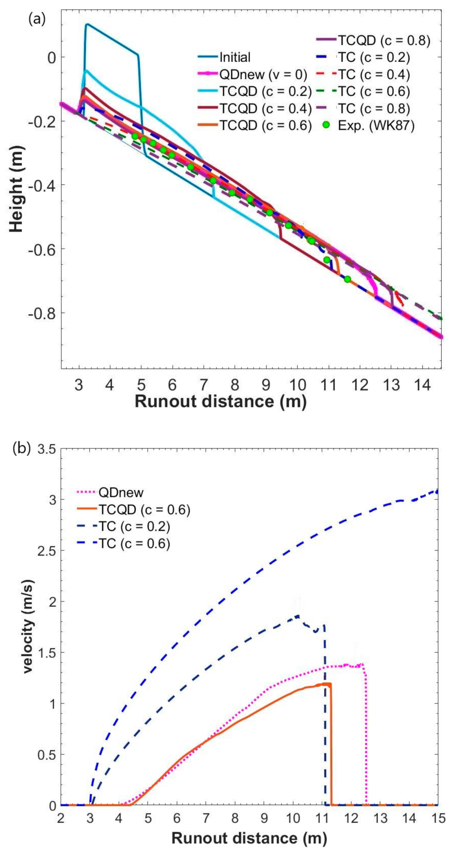
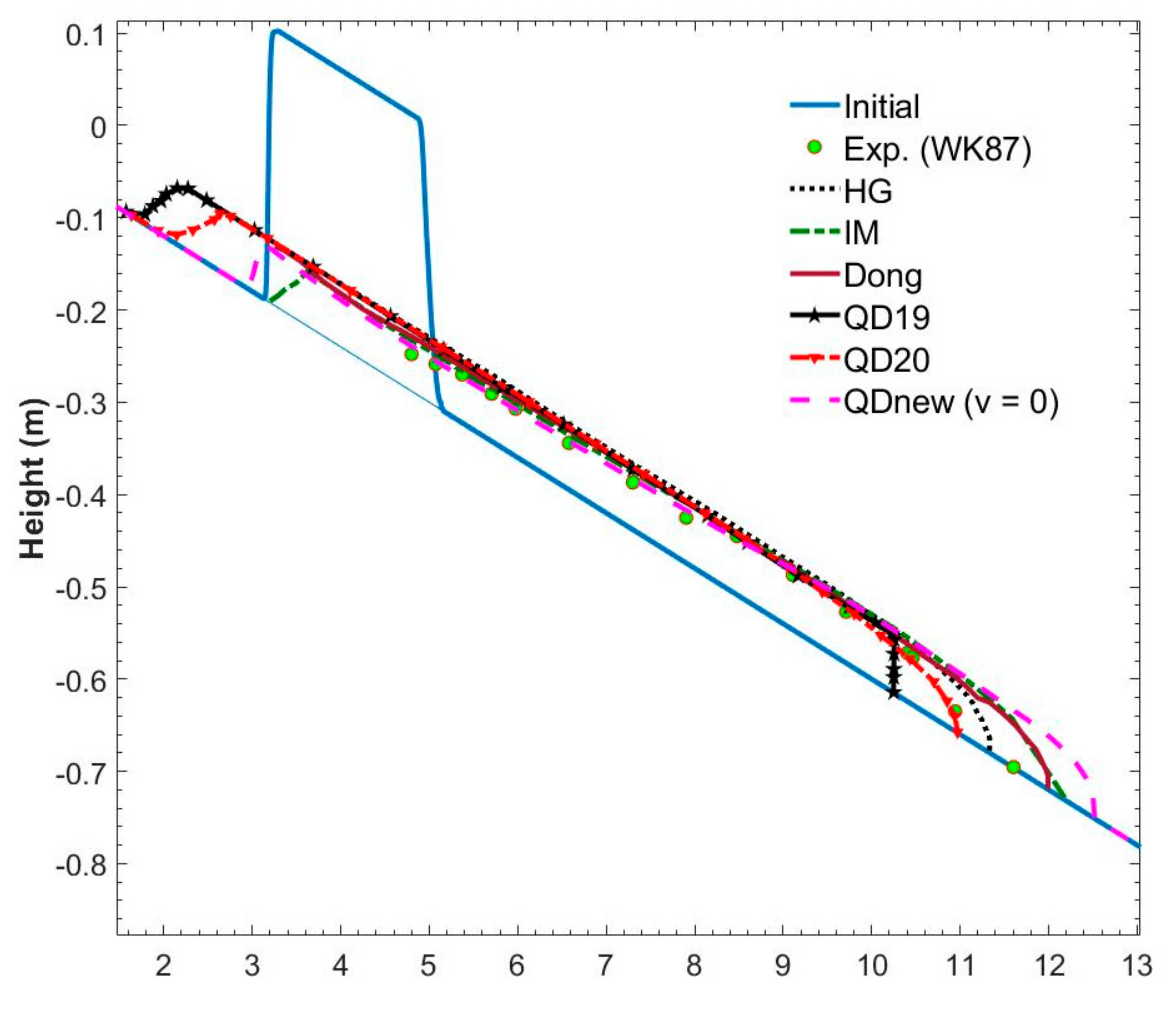
3.2. Verification with One-Dimensional Laboratory Test (Subaerial)

The three numerical models (QDnew, TC, and TCQD) were first validated using the experimental data by Wright and Krone [34], which has been previously described (case WK87). Since the width of the failure mass was not known, we, therefore, firstly set the velocity at transverse direction equal to zero (v = 0), thereby making the model QDnew one-dimensional (1D). The ability to reproduce the same results by using different widths indicated the correctness of our code. The result from QDnew (1D) was compared with experimental data and results from other 1D models e.g., [1,3,7,8] at 4.1 s, and this is shown in Figure 1. Observation from the figure showed that QDnew overpredicted the runout distance compared to the experimental data. This was similar to the results obtained by Imran et al. [3] and Dong et al. [46]. The longer runout distance was likely due to the absence of backflow, which could have reduced the frontal distance. This reason was also given by Imran et al. [3] and Dong et al. [46]. Huang and Garcia [8], on the other hand, produced a closer result with the runout distance of the experimental data, even though they suggested some slurry could be attached to the walls of the flume and not joined to the debris flow, thereby causing the slight overprediction of their result. Additionally, included in Figure 1 are solutions from literature (Qian and Das [7], QD19 (time not stated); Qian et al. [1], QD20 at 120 s). Results from QD19 and QD20 underpredicted the runout distance of the experimental data. This could be a result of the assumed width used by their study, which might be insufficient to push the flow far enough, not forgetting that numerical models are sensitive to the geometry of initial mass. Additionally, the underprediction of the runout distance by QD19 and QD20 could be due to the protracted backflow in their result. The result from QD19 has a larger backflow and much shorter runout distance compared to QD20 with a lesser backflow since it is an improved model of the former. This was likely responsible for the longer runout distance of QD20 compared to QD19. Despite the little numerical differences observed between our numerical result and the experimental data, this solution still reasonably agreed with the experimental data.
We also decided to use TC and TCQD to repeat the model run while setting their velocity in the transverse direction to zero, thereby making them also 1D models, and setting the bed as fixed, which, therefore, made the flow only depositional. However, when applying TCQD and TC, the initial concentration of the debris should be specified. Previous works did not present this information, and most other researchers who simulated this experiment did so with an assumption of constant concentration and density [1,4,7,8,46]. Since different density values of bentonite, which could be used for a back-calculation of the concentration, were found in different studies, and to avoid this, a sensitivity analysis was justified. Therefore, a sensitivity analysis was conducted with concentration values of 0.2, 0.4, 0.6, and 0.8. Using the initial failure mass parameters in TCQD, TC was also used to run the same case. Since TC did not use the Herschel–Bulkley model for bed shear stress estimation but rather used the bed shear velocity and a drag coefficient c D , a value had to be set for c D .   We, therefore, used 0.003.
Results from the sensitivity analysis of concentration using TC and TCQD were compared with experimental data and QDnew results in Figure 2a. The figure shows that concentrations of 0.2 and 0.4 underpredicted the runout distance at 4.1 s for TCQD. Since sediments drive a flow and the runout was underpredicted, it was likely the concentrations might not have been adequate to drive this flow fast enough within the experimental time to meet the runout distance of the experimental data. This, therefore, justified a higher concentration of 0.6 and 0.8. A concentration of 0.8, however, excessively overpredicted the runout distance, while a concentration of 0.6 showed a closer result with the experimental data, even though a slight underprediction was observed, which could be as a result of limited backflow of the simulation run or deposition of debris materials during the flow.
Even though we did not know the concentration used in the experimental data, we cannot, therefore, conclude that the concentration was 0.6. However, we tentatively accepted a concentration of 0.6 for this study. On the other hand, for the model TC, concentrations of 0.4, 0.6, and 0.8 significantly overpredicted the runout distance. Rather, a concentration of 0.2 was adequate to produce a runout distance similar to the experimental data. This drove us to the conclusion that a lower concentration of a turbidity current is sufficient to reach the same runout distance of a debris flow with a higher concentration, even though we could not conclude that a concentration of 0.2 was adequate since yield stress was neglected in its dynamics.
Additionally, from Figure 2a, a significant difference is observed in the results produced by QDnew and TCQD. Even though they both had the same initial geometry failure, the runout distance of debris for TCQD was lesser than that of QDnew. This was due to the presence of the bed deformation equation, whereby sediments in TCQD can be deposited since the bed was assumed to be only depositional, compared to QDnew, where the materials could not get deposited or eroded due to the lack of bed deformation equation. However, the flow tail still maintained its height with that of QDnew based on the influence of the critical height.
On the other hand, there was some similarity between TC, which represented a turbidity current model, and TCQD, a debris model in terms of material volume. While they had different bed shear stress estimations, they shared the ability to impart the bed during flow due to the coupling of the bed deformation equation. This, therefore, gave them the ability to deposit during the flow. From the observations of the results produced by TC and TCQD, there were some physical differences, as seen in Figure 2a. TC was seen to head much farther than the other model results. This was expected since a turbidity current flow is not controlled by yield stress, that is, zero yield stress, facilitating a higher runout distance as a result of reduced shear stress, and a zero dynamic viscosity, which facilitated a higher flow speed compared to that of debris flow and its rheology. Additionally, the critical height came into play, whereby the flow tail of the TC model was significantly reduced in height and even touched the bed, unlike the debris models, whereby when they reached a particular height (critical height), the height remained in equilibrium, and flow front came to a complete stop if there were no more debris materials to transport, rather than reducing the critical height. The turbidity current, instead, would rather keep reducing in height to sustain the flow, unlike a debris flow. This highlights a major difference between a turbidity current and a debris flow. Figure 2b shows a comparison between the velocity profiles of QDnew, TCQD (c = 0.6), and TC (c = 0.2, c = 0.6) at 4.1 s. A significant difference was observed between the debris models and the turbidity current model. The TC model had a higher flow velocity at both concentrations of 0.2 and 0.6, which was likely a result of zero yield stress and viscosity as explained earlier, even though TC (c = 0.6) produced an excessively higher velocity, confirming the impact of the absence of yield stress and viscosity in the modeling of debris flows. This showed that the TC model treated the flow like a Newtonian fluid while QDnew and TCQD treated it as a non-Newtonian fluid.
QDnew, on the other hand, had a higher velocity than TCQD since it had more materials to transport and sustain the flow, while TCQD was depositing its materials and leading to early loss of momentum in the flow. Table 1 shows the percentage overestimation and underestimation by the models QDnew, TCQD and TC against the experimental data. Analytically, QDnew had an overestimation of about 7.9% and TCQD underestimated by 2.4%, while TC overestimated the experimental data by about 29.3% (see Table 1).

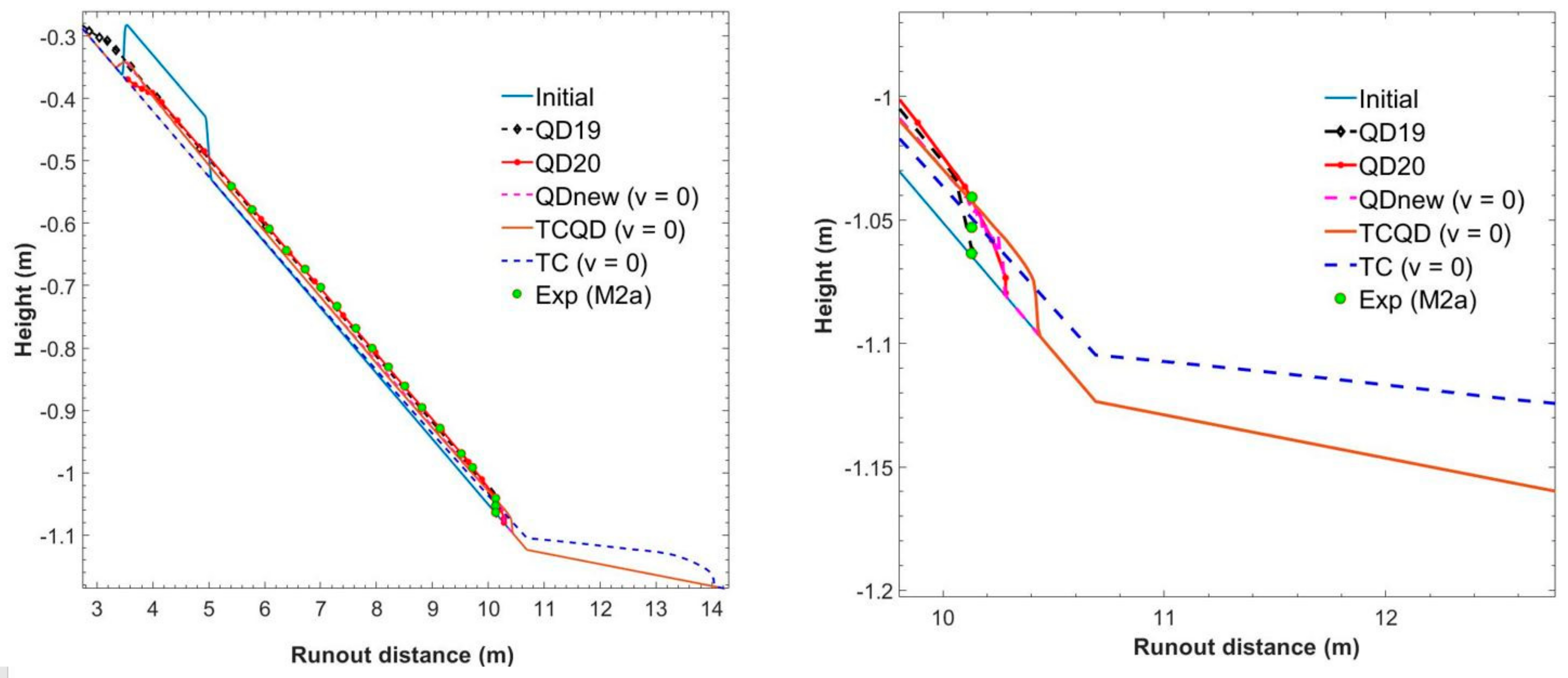
3.3. Verification with One-Dimensional Laboratory Test

The models (TC, QDnew, and TCQD) were further tested against experimental data from Mohrig et al. [35] (case M2a and M3a). For this study, a tentative concentration of 0.4 was used for the TCQD and TC models. We also set the cross-sectional velocity of the models to be zero, thereby making the three models one-dimensional. Since the initial failure geometry of the setup by Mohrig et al. [35] was unknown, except for the initial volume of 30 L for the debris, this study decided to use an initial rectangular geometry of length 1.5 m and height 0.09 m for model calibration. Since the bed used in the experiment was hard, the beds were also set to be fixed in TC and TCQD and the flow was only depositional.
Figure 3 shows the comparison of flow heights of the models with other experimental and numerical results for case M2a. As observed from Figure 3, the numerical results by QDnew and TCQD were similar and closer to the experimental data, even though a slight overprediction was observed. This difference can be a result of the nominal geometry used, which might not have been an accurate representation of the failure mass used in the experiment. Additionally, from the figure, a greater backflow was seen in results from QD19 and QD20, even though there was an improvement in QD20, showing a greater impact of gravity. This could explain why their run lasted for a longer time, of 20 s, than the experimental time, even though there was an accurate prediction of the runout distance. Further, the longer time could also be a result of the assumed initial failure geometry, which may not truly have corresponded to that of the experiment. The results produced by TC in Figure 3 show a significant difference from that of TCQD. Firstly, the result by TC produced an excessively longer runout distance despite having the same initial geometry. The larger flow deposit downslope was expected since turbidity current flow behaves like a Newtonian fluid with zero yield stress and, therefore, a higher velocity, compared to a debris flow, which behaves like a non-Newtonian fluid, thereby creating a thin flow tail and thicker flow front. Another distinct difference was the flow tail of the debris models QDnew and TCQD, which maintained the critical height, unlike that of the turbidity current model TC, which was lying on the sediment bed. Analysis showed that all the models overestimated the experimental data, and 1.48%, 3.06%, and 38.7% were, respectively, recorded for QDnew, TCQD, and TC (See Table 1).
Figure 4 shows the comparison between numerical results from our models and other experimental and numerical results for case M3a. The QDnew and TCQD models under-predicted the runout distance at a simulation time of 3.5 s, even though there was a better propagation and closer runout distance to the experimental data by TCQD, which could be a result of the positive impact of the bed deformation equation. This was likely due to the assumptions made for the initial geometry. However, there was still a significant agreement between the experimental data and the result from the models. As also seen in Figure 4, QD19 underpredicted the runout distance, and this could have been a result of a greater backflow, thereby leading to a reduced runout distance, which possibly led to the improvement of the model in QD20. QD20 from Qian et al. [1], therefore, made up for this limitation, providing a shorter backflow and reaching the exact runout distance of the experiment, even though it took a much longer time of 20 s compared to the experimental time. The result from TC, on the other hand, largely overpredicted the runout distance as a result of zero yield stress and viscosity, further confirming the impact of yield stress in a debris flow. The difference in the flow tail of turbidity current model TC and debris models QDnew and TCQD was also observed in this case.
Another significant difference between cases M2a and M3a was the propagation and runout distances of the models, whereby runout distances in the latter case crossed the slope break. Even though the same initial geometry was used in both cases and case M2a with a longer experimental time of 4.0 s, compared to the 3.5 s in case M3a, models in the latter case still produced a longer runout distance even in shorter time. This was as a result of distinct yield stresses and dynamic viscosities in both cases, as this constituted the only differences in their model settings. This could indicate that the higher the yield stress, the shorter the runout distance. Finally, QDnew underestimated the experimental data by 4.2%, TCQD also underestimated by 2.4% while TC overestimated by 12.9% (see Table 1).

4. Model Application

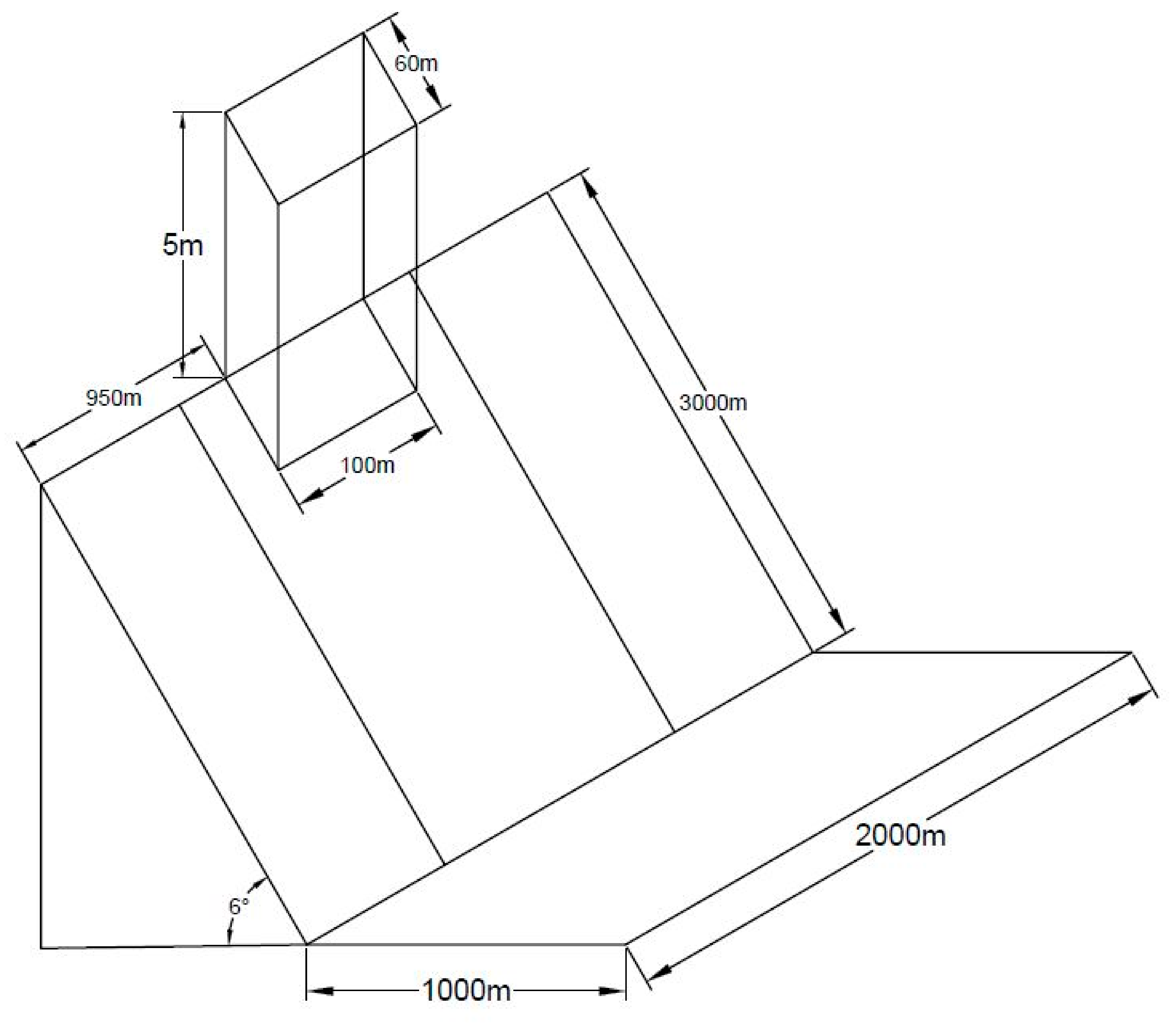
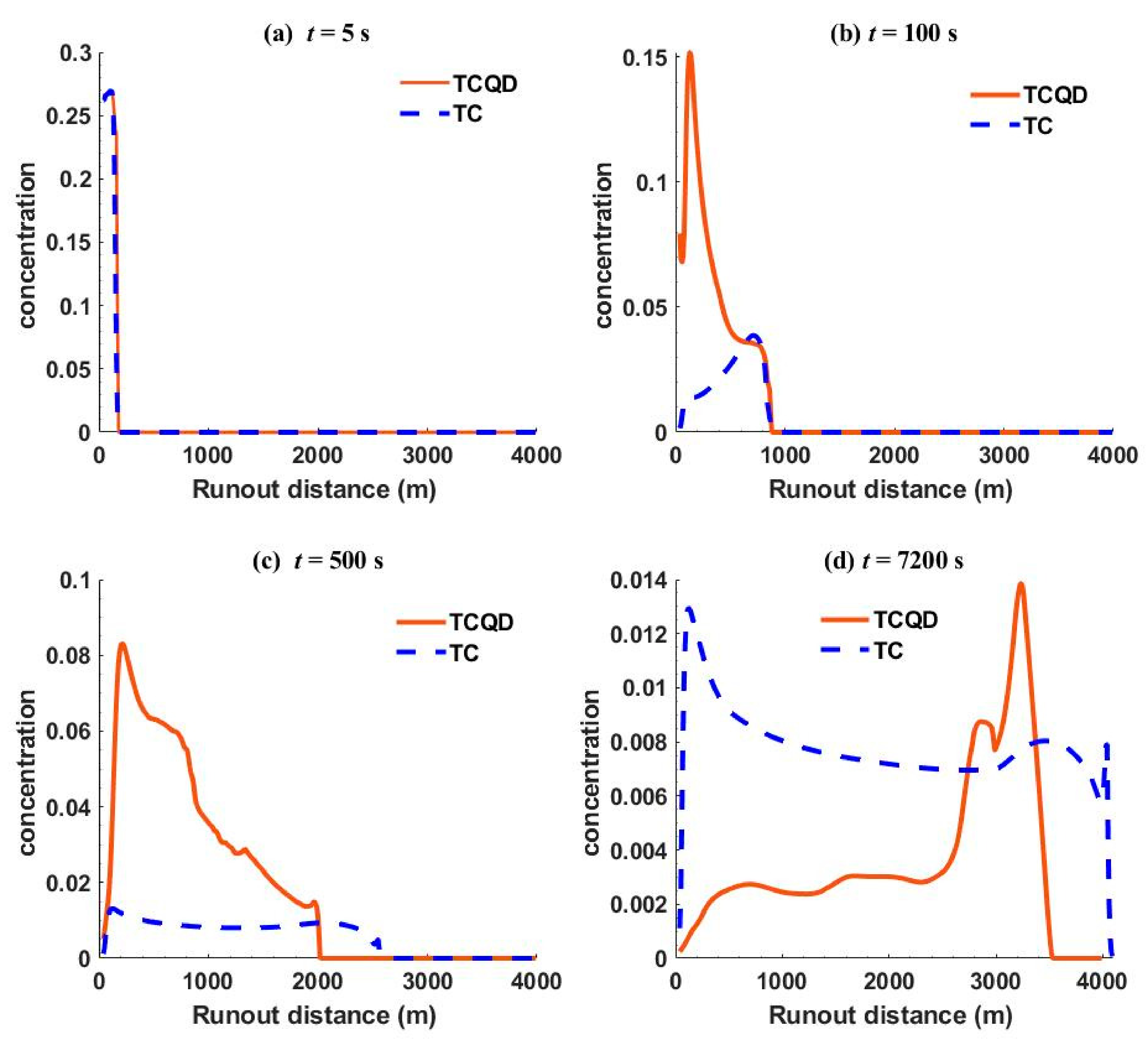
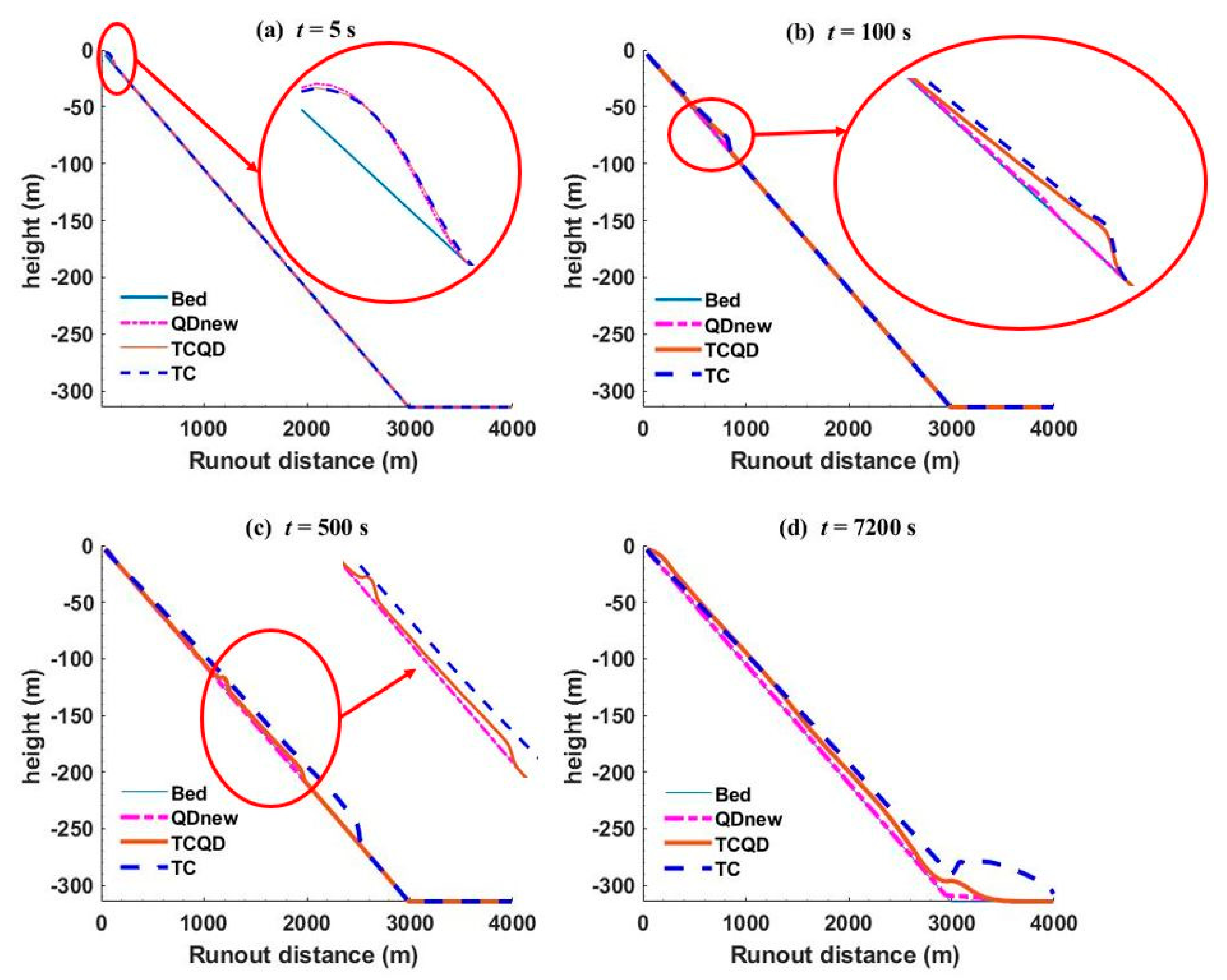
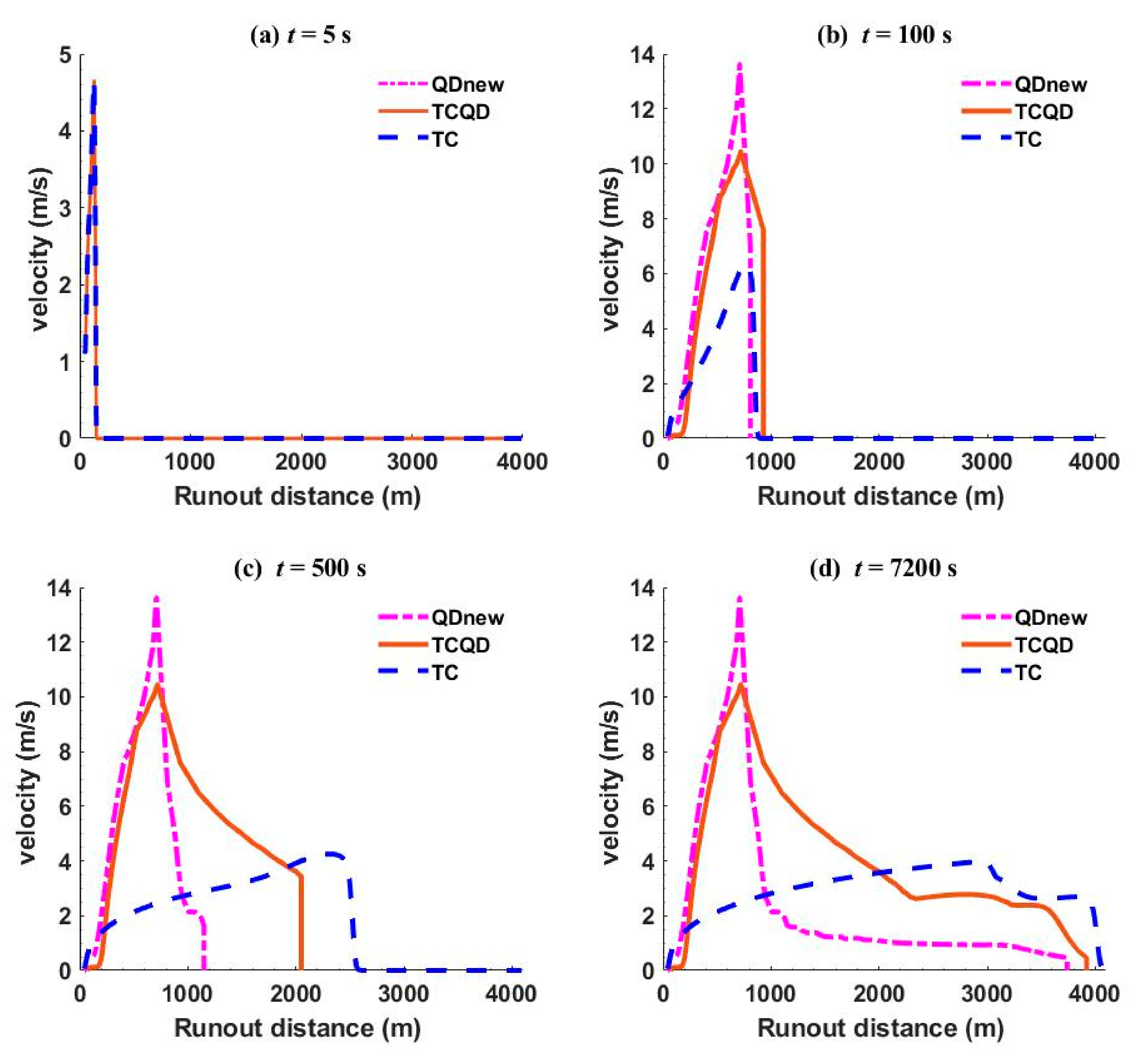
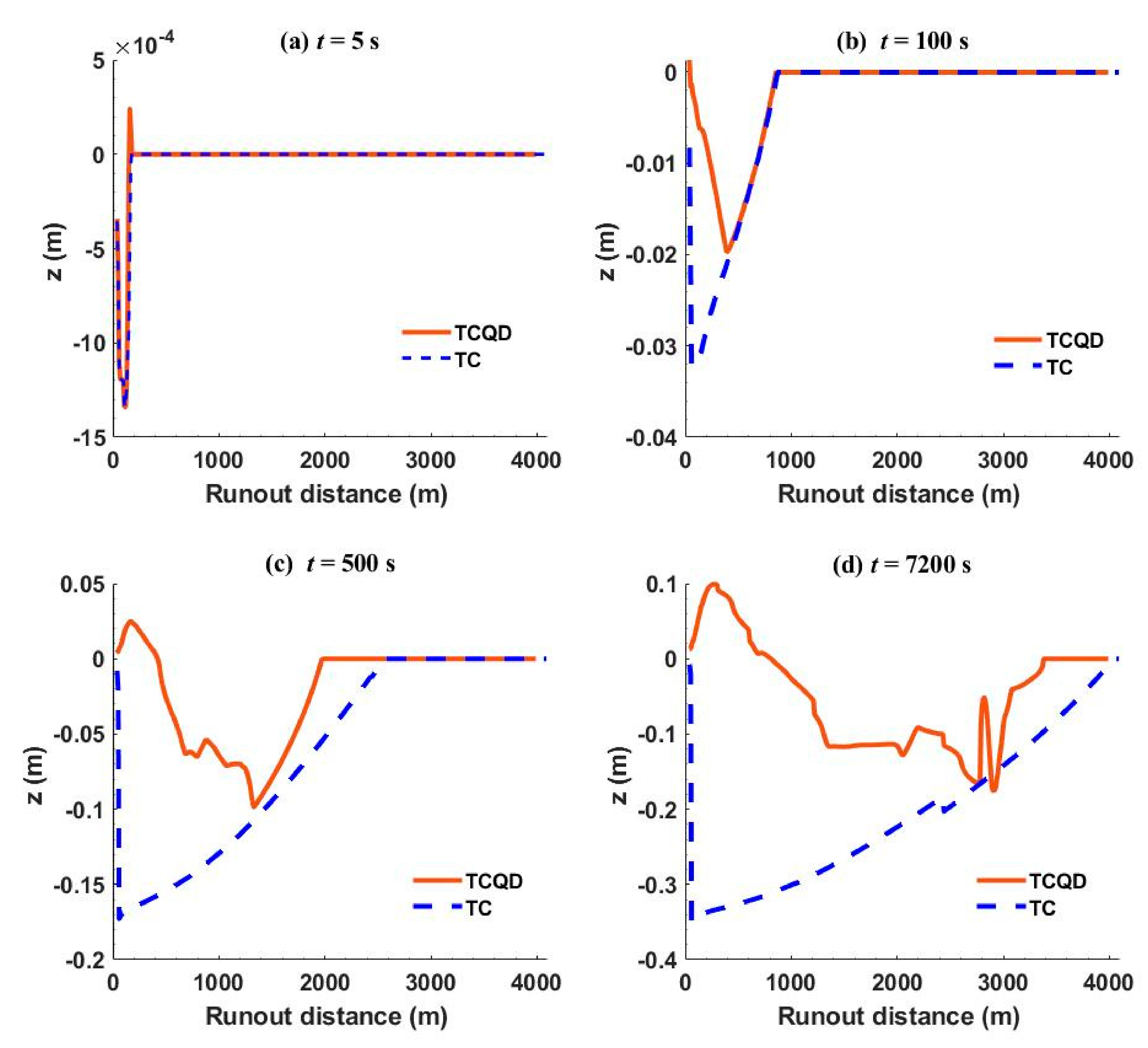
4.1. Application to Debris Flow over a Continental Shelf that Leads to Deep Sea

To further exhibit the importance of the bed deformation, models QDnew, TC, and TCQD were applied to debris flow propagation over a schematized continental shelf that leads to the deep sea (Figure 5). The distance along the shoreline was 4000 m, while across the shoreline was 2000 m. The slope angle was set as 6° at 3000 m from the start of the shelf and the deposition bed was set as flat (0°) for the remaining 1000 m. The length and width of the initial failure geometry were, respectively, set as 60 m and 100 m, while the height was 5 m. The debris flow was treated as a Bingham fluid with a yield stress of 100 Pa and dynamic viscosity of 20 Pa.s. The concentration of the debris was 0.27 and the density of the ambient fluid was 1000 kg/ m 3 . The total time of simulation was 7200 s.
Figure 6a–d shows the debris heights at different times for QDnew, TCQD, and TC. There was a significant difference in the morphology of debris along the slope and on the bed from the three models during the simulation time. Firstly, for 5 s, the debris flow for the three models crashed under the influence of gravity and reached the same runout distance (Figure 6a) since they had the same initial geometry and the influence of bed deformation may not have been significant enough at that particular time. However, as the flow progressed and at time 100 s (Figure 6b), the TCQD and TC models were far ahead and almost at the same runout distance with a considerable amount of debris materials at the flow front, while the QDnew model was much behind with lower amount of debris materials. At time 500 s (Figure 6c), the turbidity current model TC went much farther downslope and TCQD was some meters behind, while QDnew was almost lying flat on the bed even as it progressed slowly, which was likely due to a lower amount of materials since it lacked bed interaction. The longest runout distance of TC at 500 s also confirmed the findings of Huang and Garcia [8], which indicated that a flow without yield stress was faster and could experience a longer runout distance than a typical debris flow influenced by yield stress. Finally, at 7200 s (Figure 6d), the debris materials arrived at the deposition bed for the three models, however, with a significant difference in the amount of deposit. The turbidity current model had the largest amount of materials, while the QDnew model had the lowest, showing a change in the amount of debris materials at the start and the end of the flow. The incorporation of more sediments into a debris flow emphasized the importance of the bed deformation equation, even though a turbidity current may have had more influence on the bed than a debris flow. Debris deposition by the three models after the slope break also gave us some information about debris flow and turbidity currents. Distinct features were seen at the deposition bed, which was likely due to the influence of the slope break. Since the steep slope sharply reduced to zero, this affected the momentum of the onrushing debris flow. In the case of QDnew and TCQD, immediately as the flows reached the deposition bed, all momentum was lost, causing very slow movement or creeping, which eventually led to a complete stop, as defined by the debris rheology governed by yield stress and dynamic viscosity. The implication of this on bed facilities is quite significant. This can lead to a deep burial of facilities due to thick deposits, which, in turn, can cause an increase in pressure and may cause the breaking or destruction of these facilities. The turbidity current model TC, on the other hand, allowed for the spreading of bed materials. Since it was not governed by yield stress and viscosity, the momentum was not completely lost on the deposition bed, and the more the deposit transported downslope, the more the spreading or area of deposit on the deposition bed. This can also lead to the burial of bed facilities. Further, there may be some advantages in their deposition, which could include the formation of hydrocarbon after so many years. Since this was not the focus of our study, we reserved it for future study.
The velocity profiles for the three models at different times are shown in Figure 7a–d. From Figure 7a, the three models experienced a sharp increase in velocity to about 4.5 m/s due to the influence of gravity causing a crashing of the debris. This could explain the same runout distance experienced at 5 s. However, at time 100 s (Figure 7b), the debris models QDnew and TCQD still had a significant increase in their velocity, respective to about 14 m/s and 10 m/s, while the turbidity current flow had an insignificant increase despite having a longer runout distance as TCQD. The lower velocity of the TCQD and TC models compared to the QDnew model could be as a result of more materials being transported by them as a result of the interaction with the bed leading to more resistance to flow, but a sustained flow. As the flow progressed at 500 s (Figure 7c), there was a sharp decrease in the velocity of QDnew and TCQD since the debris was getting settled and the shear resistance was getting higher, while TC still experienced a slight increase. The decrease by QDnew was sharper since it had less material than TCQD and could only support consistency in flow as long as materials were available for transport. Finally, at 7200 s (Figure 7d), the debris models already lost most of their momentum and were slowing down. Since TCQD carried more materials due to the bed interaction ability, the velocity was quite higher than that of QDnew with no bed interaction ability. TC, on the other hand, was also experiencing a gradual drop in velocity since there was a slope break, though not as sharp as the debris models, and thereby allowing further spreading of sediments on the bed (Figure 7d) compared to the debris models where their deposition was vertically oriented, that is, an increase in deposit thickness.
The concentration profiles by TC and TCQD at different times are shown in Figure 8a–d. At the start of flow when the time was 5 s, the debris was just experiencing a crash and the spreading or differences were not significant enough. However, at 100 s and 500 s (Figure 8b,c), the sediments spread farther downslope, even though the spreading was more prevalent in TC than TCQD, since the rheology of TCQD facilitated higher shear resistance than TC with a lower shear resistance. Finally, at 7200 s (Figure 8d), the sediments were deposited and the higher concentration for TCQD was seen at the slope break, which could have been a result of the stoppage of flow confirming vertically oriented deposition, while TC had sediments spreading as the flow progressed along the deposition bed, indicating horizontally oriented deposition.
Finally, the bed profiles of TC and TCQD for different times are shown in Figure 9a–d. This signified the importance of the bed deformation equation in TC and TCQD, which was lacking in QDnew. The scoured depths at 5 s (Figure 9a) were similar since the flow had just started, with very minimal bed changes. However, there was a considerable difference as the flow progressed. At 100 s of the flow (Figure 9b), both models experienced significant erosion, even though erosion was more rampant in TC than TCQD. The erosion pattern of TC looked regular, as the greatest erosion occurred at the flow tail, while that of TCQD was irregular, whereby the erosion was strongest at the flow front with a haggard pattern. As the flow approached 7200 s (Figure 9d), there was considerable deposition at the flow tail of the debris flow for TCQD compared to the flow tail at 500 s, which indicated that the debris was getting fully deposited due to loss of momentum as it approached the flat bed. Additionally, both erosions in the models TC and TCQD at this time experienced a decrease in erosion and more deposition since the bed was getting gentle. The erosion phenomenon is one of the dangers associated with debris flow, which can lead to the exposure of materials on the sea bed and as well their destruction. Therefore, our observations stressed the importance of the bed deformation equation in the modeling of debris flows, and this study reasonably proved that a debris flow can be erosional and depositional.

4.2. Sensitivity Analyses

The model TCQD was further used to carry out a sensitivity analysis to test the impact of several parameters on the deformation of the sediment bed using the geometry of the continental shelf in Figure 7. The parameters used in the model application served as a reference case and were labeled case 1 in Table 2. Cases 2 and 3 showed the impact of sediment size on the bed while cases 4 and 5 illustrated the influence of the slope angle on the bed. Further, cases 6 and 7 showed the influence of the bed porosity while cases 8 and 9 gave more information on how the concentration of debris (mass, density) can impart the bed.

4.2.1. Impact of Sediment Size and Bed Slope Angle on Bed Thickness

Figure 10a shows the result of the different sediment sizes of 37 µm, 50 µm, and 100 µm, representing cases 1–3. The findings showed that the bed sediment sizes had a strong influence on the erosion and deformation of the bed. The bed with the highest sediment size, that is, case 3, which was made of coarse particles (100 µm), had the highest scoured depth compared to finer sediment size (37 µm, case 1), which had the least scoured depth. This could be a result of the high-speed condition that defines the value of the erosion coefficient. When the speed of the debris was high, the erosion coefficient can be insensitive to the sediment size and the coefficient would be determined by the speed of the flow (Equations (11) and (12)). On the other hand, the net sediment change flux (Equation (10)) was directly influenced by the sediment size. Therefore, the flow with higher particle size was more entrained, which may even lead to more erosion of sediment than the entrainment by water. According to Gauer and Issler [47], the erosion speed increases with an increase in particle size. Davies and McSaveney [48] recommended that smaller particle sizes of bed sediments should not be used for erodible beds in experimental investigations as the materials become too fine, leading to a high basal resistance that prevents entrainment and could even generate great dust instead. Additionally, Iverson et al. [49] explained that large cohesion (finer sediments) of sediment beds could lead to higher shear resistance, which causes lesser erosion. Therefore, larger bed particles should be used to study the entrainment property of a flow. From this particular observation, the size of sediment plays a very important role in how much the bed is affected during a debris flow.
Different bed slope angles of 3°, 6°, and 9°, representing cases 4, 5, and 1, respectively, were also compared in Figure 10b. The findings (Figure 10b) showed that the steepest slope (9°, case 5) had the deepest scoured depth through the flow time compared to the gentlest slope (3°, case 4), which only experienced deposition since it could only move for some few meters. This indicated that the steeper the slope, the more dangerous a debris flow can be. The result also showed that the gentlest slope had the shortest runout distance. This could be easily explained. A debris flow over a steeper bed slope (9°) is expected to be faster since gravity impact will be higher and therefore, a longer runout distance compared to a gentle slope where gravity impact is limited. In fact, the debris along the 3° slope barely moved away from the starting point. This indicated that the bottom slope had a direct relationship with the runout distance, whereby the steeper the bottom slope, the longer the runout distance, and this was similar to the conclusion of Qian and Das [7].

4.2.2. Impact of Bed Porosity and Debris Concentration on Bed Thickness

Another important factor that determines the weakness of the bed and vulnerability to erosion is the bed porosity. Porosities of 0.2, 0.5, and 0.7 representing cases 6, 1, and 7, respectively, were also compared to test the bed failure against a debris flow, and the result is shown in Figure 10c. The findings showed that the higher the porosity of the bed, the greater the tendency to bed failure, and the deeper the bed scouring depth. A mild porosity of 0.2 (case 6) showed a lesser scouring depth, making the bed less affected by debris flow. This indicated that the more the bed materials are loose, the more they can be eroded. This agreed with the opinions of several researchers. When the substrate is loose, the intense impact can erode a large amount of bed materials [16]. Reid et al. [50], in their study, proved that wetter bed sediment allows for more erosion compared to a drier bed. They further claimed that the pore pressure in bed sediment causes a disturbance in the stress state and the structure of soils, which could lead to a reduction in shear strength, and thereby aid erosion. When the substrate is saturated, should a debris flow collide intensely, the substrate becomes liquefied under impact loading, and this may significantly reduce the shear resistance of the bed materials [51,52]. Therefore, bed porosity plays a strong role in how much the bed will be scoured during a debris flow.
The debris concentration, that is, mass and density, is also a major factor that should be considered in the flow of debris. Due to a difference in the solid volume fraction between the bed and the debris flow, the concentration of the body tends to vary by eroding more materials [53]. Therefore, this study did a comparison on the effect of different concentrations (0.27, 0.5, and 0.8, representing cases 1, 8, and 9, respectively) on the bed, and the result is shown in Figure 10d. The result showed a significant difference made by different concentrations on the sediment bed after a debris flow. Since concentration is directly proportional to mass and density, the results showed that the higher the mass of debris, the deeper it can scour, indicating higher strength and energy for debris transport. Further, the more it scours, the more the bed sediments it incorporates into its flow. This, therefore, makes the flow travel a longer distance and time, since it has more materials to move or sustain the flow, and the more sediment volume that will be deposited at the end of the flow. This supports the claim by Liu et al. [54], who indicated that the amount of sediments in a debris flow increases with entrainment compared to that without entrainment. In an experimental investigation by Lu et al. [16], they claimed that a high debris mass enhances the entrainment effect because of greater entrainment energy, which makes the erosion process last longer.

5. Conclusions

Two-dimensional models (TCQD and QDnew) were developed from the turbidity current model (TC) to predict the movement of debris flow over subaerial and subaqueous environments. This is quite important, because of marine facilities that are laid on the sea bed, particularly pipelines and submarine cables. The models were built on the complete mass and momentum conservation laws of the water–sediment mixture and mass conservation of the sediment and bed material. TCQD and TC, which can interact with the bed, were only different through the bed shear stress formulation. While TCQD contained the effect of yield stress and dynamic viscosity on the debris model, this was lacking in TC. Additionally, QDnew was a simplified form of TCQD, whereby erosion and deposition were ignored in the former, while these were considered in the latter. The models were first validated against experimental investigations (Wright and Krone [36]; Mohrig et al. [23]). The three models (QDnew, TCQD, and TC) were then applied to a schematic continental shelf that led to the deep sea with feedback of bed deformation. TC and TCQD showed a significant bed degradation through the flow, which, therefore, led to a large number of thick deposits compared to the initial volume, even though TC had a horizontally oriented deposit while TCQD had a vertically oriented deposit. QDnew, on the other hand, had the lowest deposit since it could not entrain materials and, therefore, no change in volume of debris materials. A sensitivity analysis was then carried out to find the impact of bed parameters on the evolution of the bed during a debris flow. Findings showed that bed sediment size, bed slope, concentration (mass and density) of debris, and bed porosity play a very significant role in how deep a bed is scoured during a debris flow, with all of the factors showing a positive correlation. This study is, therefore, able to numerically show the impact of erosion and deposition on a debris flow.

Author Contributions

Conceptualization, P.H.; Methodology, P.H., and A.A.A.; Resources, P.H.; Investigation, P.H., A.A.A. All authors have read and agreed to the published version of the manuscript.

Funding

This research was funded by the National Natural Science Foundation of China (No. 11772300; 11872332), the Zhejiang Natural Science Foundation (No. LR19E090002), and the HPC Center OF ZJU (ZHOUSHAN CAMPUS).

Institutional Review Board Statement

Not applicable.

Informed Consent Statement

Not applicable.

Data Availability Statement

Not applicable.

Conflicts of Interest

The authors declare no conflict of interest.

References

  1. Qian, X.; Xu, J.; Das, H.S.; Wang, D.; Bai, Y. Improved Modeling of Subaerial and Subaqueous Muddy Debris Flows. J. Hydraul. Eng. 2020, 146, 06020007. [Google Scholar] [CrossRef]
  2. De Blasio, F.V. Hydroplaning and submarine debris flows. J. Geophys. Res. 2004, 109. [Google Scholar] [CrossRef]
  3. Imran, J.; Parker, G.; Locat, J.; Lee, H. 1D numerical model of muddy subaqueous and subaerial debris flows. J. Hydraul. Eng. 2001, 27, 717–729. [Google Scholar] [CrossRef]
  4. Kim, J.; Løvholt, F.; Issler, D.; Forsberg., C.F. Landslide material control on tsunami genesis—The Storegga Slide and tsunami (8,100 years BP). J. Geophys. Res. Oceans 2019, 124, 3607–3627. [Google Scholar] [CrossRef] [Green Version]
  5. McDougall, S.; Hungr, O. A model for the analysis of rapid landslide motion across three-dimensional terrain. Can. Geotech. J. 2004, 41, 1084–1097. [Google Scholar] [CrossRef]
  6. Pastor, M.; Quecedo, M.; González, E.; Herreros, I.; Fernández Merodo, J.A.; Mira, P. A simple approximation to bottom friction for Bingham fluid depth integrated models. J. Hydraul. Eng. 2004, 130, 149–155. [Google Scholar] [CrossRef]
  7. Qian, X.; Das, H.S. Modeling Subaqueous and Subaerial Muddy Debris Flows. J. Hydraul. Eng. 2019, 145, 04018083. [Google Scholar] [CrossRef]
  8. Huang, X.; García, M.H.; Huang, X.; García, M.H. A Perturbation Solution for Bingham-Plastic Mudflows. J. Hydraul. Eng. 1997, 123, 986–994. [Google Scholar] [CrossRef]
  9. Pastor, M.; Blanc, T.; Haddad, B.; Petrone, S.; Sanchez Morles, M.; Drempetic, V.; Issler, D.; Crosta, G.B.; Cascini, L.; Sorbino, G.; et al. Application of a SPH depth-integrated model to landslide run-out analysis. Landslides 2004, 11, 793–812. [Google Scholar] [CrossRef] [Green Version]
  10. Pudasaini, S.P. A general two-phase debris flow model. J. Geophys. Res. Earth Surf. 2012, 117, F03010. [Google Scholar] [CrossRef]
  11. Meng, X.; Wang, Y. Investigations of Gravity-Driven Two-Phase Debris Flows. In Recent Advances in Modeling Landslides and Debris Flows; Springer Series in Geomechanics and Geoengineering; Wu, W., Ed.; Springer: Cham, Switzerland, 2015. [Google Scholar] [CrossRef]
  12. Wang, W.; Chen, G.; Han, Z.; Zhou, S.; Zhang, H.; Jing, P. 3D numerical simulation of debris-flow motion using SPH method incorporating non-Newtonian fluid behavior. Nat Hazards 2016, 81, 1981–1998. [Google Scholar] [CrossRef]
  13. Braun, A.; Cuomo, S.; Petrosino, S.; Wang, X.; Zhang, L. Numerical SPH analysis of debris flow run-out and related river damming scenarios for a local case study in SW China. Landslides 2018, 15, 535–550. [Google Scholar] [CrossRef]
  14. Brufau, P.; Garcia-Navarro, P.; Ghilardi, P.; Natale, L.; Savi, F. 1D mathematical modeling of debris flow. J. Hydraul. Res. 2000, 38, 435–446. [Google Scholar] [CrossRef]
  15. Zhou, G.G.D.; Du, J.; Song, D. Numerical study of granular debris flow run-up against slit dams by discrete element method. Landslides 2020, 17, 585–595. [Google Scholar] [CrossRef]
  16. Lu, P.; Yang, X.; Xu, F.; Hou, T.; Zhou, J. An Analysis of the Entrainment Effect of Dry Debris Avalanches on Loose Bed Materials; SpringerPlus: Cham, Switzerland, 2016; pp. 1–15. [Google Scholar]
  17. Toniolo, H.; Harff, P.; Marr, J.; Paola, C.; Parker, G. Experiments on reworking by successive unconfined subaqueous and subaerial muddy debris flows. J. Hydraul. Eng. 2004, 130, 38–48. [Google Scholar] [CrossRef]
  18. Takebayashi, H.; Fujita, M. Numerical Simulation of a Debris Flow on the Basis of a Two-Dimensional Continuum Body Model. Geosciences 2020, 10, 45. [Google Scholar] [CrossRef] [Green Version]
  19. Ali, S.Z.; Dey, S. Origin of the scaling laws of sediment transport. Proc. R. Soc. A 2017, 473, 20160785. [Google Scholar] [CrossRef]
  20. Ali, S.Z.; Dey, S. Impact of phenomenological theory of turbulence on pragmatic approach to fluvial hydraulics. Phys. Fluids 2018, 30, 045105. [Google Scholar] [CrossRef]
  21. Venditti, J.G.; Church, M.; Bennett, S.J. On interfacial instability as a cause of transverse subcritical bed forms. Water Resour. Res. 2006, 42, W07423. [Google Scholar] [CrossRef] [Green Version]
  22. Dey, S. Fluvial Hydrodynamics: Hydrodynamic and Sediment Transport Phenomena; Springer: Berlin, Germany, 2014. [Google Scholar]
  23. Naqshband, S.; Ribberink, J.S.; Hurther, D.; Hulscher, S.J.M.H. Bed load and suspended load contributions to migrating sand dunes in equilibrium. J. Geophys. Res. Earth Surf. 2014, 119, 1043–1063. [Google Scholar] [CrossRef] [Green Version]
  24. Ourmières, Y.; Chaplin, J.R. Visualizations of the disturbed-laminar waveinduced flow above a rippled bed. Exp. Fluids 2004, 36, 908–918. [Google Scholar] [CrossRef]
  25. Recking, A.; Bacchi, V.; Naaim, M.; Frey, P. Antidunes on steep slopes. J. Geophys. Res. Earth Surf. 2009, 114, F04025. [Google Scholar] [CrossRef]
  26. Eekhout, J.P.C.; Hoitink, A.J.F.; Mosselman, E. Field experiment on alternate bar development in a straight sand-bed stream. Water Resour. Res. 2013, 49, 8357–8369. [Google Scholar] [CrossRef]
  27. Li, J.; Cao, Z.; Pender, G.; Liu, Q. A double layer-averaged model for dam-break flows over mobile bed. J. Hydraul. Res. 2013, 51, 518–534. [Google Scholar] [CrossRef] [Green Version]
  28. O’Brien, J.S.; Julien, P.J.; Fullerton, W.T. Two-dimensional water flood and mudflow simulation. J. Hyd. Eng. 1993, 119, 244. [Google Scholar] [CrossRef]
  29. Egashira, S.; Miyamoto, K.; Takahiro, I. Constitutive Equations of Debris Flows and Their Applicability. In Debris Flow Hazard Mitigation: Mechanics, Prediction and Assessment; ASCE: New York, NY, USA, 1997; pp. 340–349. [Google Scholar]
  30. Takahashi, T. Debris Flow. Annu. Rev. Fluid Mech. 1981, 13, 57–77. [Google Scholar] [CrossRef]
  31. Armanini, A.; Fraccarollo, L. Critical Conditions for Debris Flow. In Debris Flow Hazard Mitigation: Mechanics, Prediction, and Assessment; ASCE: New York, NY, USA, 1997; pp. 434–443. [Google Scholar]
  32. Hirano, M.; Harada, T.; Banihabib, M.E.; Kawahara, K. Estimation of Hazard Area Due to Debris Flow”, Debris Flow Hazard Mitigation: Mechanics, Prediction and Assessment; ASCE: San Francisco, CA, USA, 1997; pp. 697–706. [Google Scholar]
  33. Hu, P.; Cao, Z.; Pender, G. Well-balanced two-dimensional coupled modelling of submarine turbidity currents. In Maritime Engineering, Proceedings of the Institute of Civil Engineers; ICE Publishing: London, UK, 2012; Volume 165, pp. 169–188. [Google Scholar]
  34. Wright, V.; Krone, R.B. Laboratory and Numerical Study of Mud and Debris Flow; Rep. 1 and 2; Department of Civil Engineering, University of California: Davis, CA, USA, 1987. [Google Scholar]
  35. Mohrig, D.; Elverhøi, A.; Parker, G. Experiments on the relative mobility of muddy subaqueous and subaerial debris flows, and their capacity to remobilize antecedent deposits. Mar. Geol. 1999, 154, 117–129. [Google Scholar] [CrossRef]
  36. Hu, P.; Cao, Z.; Pender, G.; Tan, G. Numerical modelling of turbidity currents in the Xiaolangdi reservoir, Yellow River, China. J. Hydrol. 2012, 464–465, 41–53. [Google Scholar] [CrossRef]
  37. Hu, P.; Li, Y. Numerical modeling of the propagation and morphological of turbidity currents using a cost-saving strategy of solution updating. Int. J. Sed. Res. 2020, 35, 587–599. [Google Scholar] [CrossRef]
  38. Fukushima, Y.; Parker, G.; Pantin, H.M. Prediction of ignitive turbidity currents in Scripps Submarine Canyon. Mar. Geol. 1985, 67, 55–81. [Google Scholar] [CrossRef]
  39. Parker, G.; Fukushima, Y.; Pantin, H.M. Self-accelerating turbidity currents. J. Fluid Mech. 1986, 171, 145–181. [Google Scholar] [CrossRef]
  40. Zhang, R.J.; Xie, J.H. Sedimentation Research in China-Systematic Selections; China Water and Power Press: Beijing, China, 1993. [Google Scholar]
  41. Herschel, W.H.; Bulkley, R. Konsistenzmessungen von Gummi-Benzollösungen (Measuring the consistency of rubber benzene solution). Kolloid Z. 1926, 39, 291–300. [Google Scholar] [CrossRef]
  42. Marr, J.G.; Elverhoi, A.; Harbitz, C.; Imran, J.; Harff, P. Numerical simulation of mud-rich subaqueous debris flows on the glacially active margins of the Svalbard-Barents Sea. Mar. Geol. 2002, 188, 351–364. [Google Scholar] [CrossRef]
  43. Parsons, J.D.; Friedrichs, C.T.; Traykovski, P.A.; Mohrig, D.; Imran, J.; Syvitski, J.P.M.; Parker, G.; Puig, P.; Buttles, J.L.; García, M.H. The mechanics of marine sediment gravity flows. In Continental Margin Sedimentation: From Sediment Transport to Sequence Stratigraphy; Nittrouer, C.A., Austin, J.A., Field, M.E., Kravitz, J.H., Syvitski, J.P.M., Wiberg, P.L., Eds.; Blackwell Publishing: Oxford, UK, 2007. [Google Scholar]
  44. Hu, P.; Cao, Z.X. Fully coupled mathematical modeling of turbidity currents over erodible bed. Adv. Water Res. 2009, 32, 1–15. [Google Scholar] [CrossRef]
  45. Aureli, F.; Maranzoni, A.; Mignosa, P.; Ziveri, C. A weighted surface-depth gradient method for the numerical integration of the 2D shallow-water equations with topography. Adv. Water Res. 2008, 31, 962–974. [Google Scholar] [CrossRef]
  46. Dong, Y.; Wang, D.; Lan, C. Assessment of depth-averaged method in analysing runout submarine landslide. Landslides 2019, 17, 543–555. [Google Scholar] [CrossRef]
  47. Gauer, P.; Issler, D. Possible erosion mechanisms in snow avalanches. Ann. Glaciol. 2004, 38, 384–392. [Google Scholar] [CrossRef] [Green Version]
  48. Davies, T.R.; McSaveney, M.J. Runout of dry granular avalanches. Can. Geotech. J. 1999, 36, 313–320. [Google Scholar] [CrossRef]
  49. Iverson, R.M.; Reid, M.E.; Logan, M.; LaHusen, R.G.; Godt, J.W.; Griswold, J.P. Positive feedback and momentum growth during debris-flow entrainment of wet bed sediment. Nat. Geosci. 2011, 4, 116–121. [Google Scholar] [CrossRef]
  50. Reid, M.E.; Iverson, R.M.; Logan, M.; LaHusen, R.G.; Godt, J.W.; Griswold, J.P. Entrainment of bed sediment by debris flows: Results from large-scale experiments. In Proceedings of the Fifth International Conference on debris flow hazards mitigation, mechanics, prediction and assessment, Padua, Italy, 14–17 June 2011; pp. 367–374. [Google Scholar]
  51. Hungr, O.; Evans, S.G. Entrainment of debris in rock avalanches: An analysis of a long run-out mechanism. Geol. Soc. Am. Bull. 2004, 116, 1240–1252. [Google Scholar] [CrossRef]
  52. Wang, G.; Sassa, K.; Fukuoka, H. Downslope volume enlargement of a debris slide-debris flow in the 1999 Hiroshima, Japan, rainstorm. Eng. Geol. 2003, 69, 309–330. [Google Scholar] [CrossRef]
  53. Pudasaini, S.P.; Fischer, J.T. A New Two-Phase Erosion-Deposition Model for Mass Flows; Geophysical Research Abstract: Vienna, Austria, 2016; Volume 18, EGU2016-4424. [Google Scholar]
  54. Liu, W.; He, S.; Chen, Z.; Yan, S.; Deng, Y. Effect of viscosity changes on the motion of debris flow by considering entrainment. J. Hydraul. Res. 2020, 59, 1–16. [Google Scholar] [CrossRef]
Figure 1. Comparison of debris-flow height between experimental, analytical, and numerical data sets for case WK87 (“Exp.” data from Wright and Krone [34]; “Analytic” data from Huang and García [8]; IM from Imran et al. [3]; Dong from Dong et al. [46]; “Num. QD19, QD20” data from Qian and Das [7], Qian et al. [1], resp.).
Water 13 01698 g001
Figure 2. (a) Sensitivity result for different concentrations using TC and TCQD and comparison of debris-flow height with experimental and numerical data sets for case WK87 (“Exp.” data from Wright and Krone [34]). (b) Velocity profiles for QDnew, TC, and TCQD.
Water 13 01698 g002
Figure 3. Comparison of debris-flow height between experimental and numerical data sets for case M2a (“Exp.” data from Mohrig et al. [23]; “Num. QD19, QD20” data from Qian and Das [7], Qian et al. [1], resp.).
Water 13 01698 g003
Figure 4. Comparison of debris-flow height between experimental and numerical data sets for case M3a (“Exp.” data from Mohrig et al. [35]; “Num. QD19, QD20” data from Qian and Das [7], Qian et al. [1], resp.).
Water 13 01698 g004
Figure 5. Schematic diagram of a continental shelf that leads to the deep sea (not drawn to scale).
Water 13 01698 g005
Figure 6. Debris heights along the slope for QDnew, TC, and TCQD at different times. (ad) show the debris flow heights at 5 s, 100 s, 500 s, and 7200 s, respectively.
Water 13 01698 g006
Figure 7. Velocity profiles of QDnew, TCQD, and TC at different times. (ad) show the velocity profiles at 5 s, 100 s, 500 s, and 7200 s, respectively.
Water 13 01698 g007
Figure 8. Concentration profiles of TCQD and TC at different times. (ad) show the concentration profiles at 5 s, 100 s, 500 s, and 7200 s, respectively.
Water 13 01698 g008
Figure 9. Bed deformation profiles of TCQD and TC at different times. (ad) show the bed deformation profiles at 5 s, 100 s, 500 s, and 7200 s, respectively.
Water 13 01698 g009
Figure 10. (d) Comparisons of the evolution of the sediment bed. (a) different sediment sizes (b) different bed slopes, (c) different slopes, and (d) different concentrations.
Water 13 01698 g010
Table 1. Summary of percentage estimation for the model performance of QDnew, TCQD, and TC.
CasesModelsEstimation (%)
WK87QDnew7.9
TCQD−2.4
TC29.3
M2aQDnew1.48
TCQD3.06
TC38.7
M3aQDnew−4.2
TCQD−2.4
TC12.9
Table 2. Summary of sensitivity analysis parameters.
Case No.d (µm)   S b   Angle   ( ° ) Porosityc τ y i e l d   ( Pa ) μ (Pa.s) Remarks
13760.50.2710020Reference case
25060.50.2710020Impact of sediment size
310060.50.2710020
43730.50.2710020Impact of bed slope angle
53790.50.2710020
63760.20.2710020Impact of bed porosity
73760.70.2710020
83760.50.510020Impact of concentration/mass/density
93760.50.810020
Publisher’s Note: MDPI stays neutral with regard to jurisdictional claims in published maps and institutional affiliations.

