Overland Flow Resistance Law under Sparse Stem Vegetation Coverage

Abstract

To explore the characteristics of overland flow resistance under the condition of sparse vegetative stem coverage and improve the basic theoretical research of overland flow, the resistance characteristics of overland flow were systematically investigated under four slope gradients (S), seven flow discharges (Q), and six degrees of vegetation coverage (Cr). The results show that the Manning roughness coefficient (n) changes with the ratio of water depth to vegetation height (h/hv) while the Reynolds number (Re), Froude number (Fr), and slope (S) are closely related to vegetation coverage. Meanwhile, h/hv, Re, and Cr have strong positive correlations with n, while Fr and S have strong negative correlations with n. Through data regression analysis, a power function relationship between n and hydraulic parameters was observed and sensitivity analysis was performed. It was concluded that the relationship between n and h/hv, Re, Cr, Q, and S shows the same law; in particular, for sparse stem vegetation coverage, Cr is the dominant factor affecting overland flow resistance under zero slope condition, while Cr is no longer the first dominant factor affecting overland flow resistance under non-zero slope condition. In the relationship between n and Fr, Cr has the least effect on overland flow resistance. This indicates that when Manning roughness coefficient is correlated with different hydraulic parameters, the same vegetation coverage has different effects on overland flow resistance. Therefore, it is necessary to study overland flow resistance under the condition of sparse stalk vegetation coverage.

1. Introduction

Overland flow is one of the causes of soil erosion and water loss. It is also the main driving factor for the migration of pollutants, sediment production, and topographic evolution [1,2,3,4]. Overland flow characteristics are mainly affected by surface coverage, slope, and flow discharge [5,6]. Vegetation plays an important role in the benign cycle of the ecological environment and has become an indispensable part of the ecological environment, so it is for the ecological slope [7,8,9,10,11,12]. Vegetation modifies the mixing effect of turbulence and dissipates the energy of overland flow, affects sediment transport and settlement, and then reduces soil erosion on slopes. Meanwhile, only when vegetation cover reaches a certain degree can the vegetation effect be prominent; if the vegetation cover is too large, the effect of vegetation will not only not increase, but the surface soil moisture and nutrients will decrease greatly due to the sharp increase of vegetation consumption, leading to soil drying and increasing soil burden. Therefore, it is necessary to clarify the change characteristics of the vegetation slope runoff resistance coefficient, reveal the hydrodynamic characteristics and dynamic erosion processes of slope runoff, and provide a scientific basis for the treatment of vegetation as it relates to soil erosion.

The presence of vegetation has significant effects on the resistance of land to overland flow [8,13,14,15,16,17,18,19]. At present, a great amount of research has been conducted on the influence of vegetation on the Manning roughness coefficient. Previous studies have mainly focused on the effects of vegetation type [20,21,22], vegetation flexibility [23], vegetation relative submergence height [24,25], and vegetation stem diameter [19,26] on the parameters of flow resistance. However, the effect of vegetation coverage on flow resistance and characteristics has also been studied, but the research premise is mostly based on larger vegetation coverage [27,28,29,30,31].

In fact, plant density plays an important role in influencing flow resistance [32]. With the continuous strengthening of research on the characteristics of resistance to overland flow, the effects of vegetation cover on flow resistance have been given an increasing amount of attention recently. Zhao et al. [19] considered that the Reynolds number (Re) for vegetated slopes was much higher than it was for bare slopes due to the influence of vegetation stems on the effective flow width and unit flow discharge. Pan and Shangguan [33] and Wu et al. [34] found that on natural slope, the vegetation stems could increase the infiltration and reduce the runoff and then weaken the soil erosion. Therefore, the Re decreased as vegetative cover increased under simulated rainfall on mobile beds. In addition, the Froude number (Fr) decreased and Manning roughness coefficient (n) increased with increased vegetative cover [19,33,35]. Nepf [36] believed that even with similar arrays and Reynolds numbers, the coefficient of flow resistance may decrease with increasing vegetation density. The experiment of Liu and Zeng [37] revealed that the Drag coefficient logarithmically increases with the vegetation density under supercritical flow, while for subcritical flow, the Drag coefficient logarithmically decreases with the vegetation density. This has also been presented by Wu et al. [38] based on limited experimental results, whom concluded that the roughness coefficients for sub- and supercritical flows have opposite trends of variation. However, Stoesser et al. [39] believed that the Drag coefficient increased with increasing vegetation density.

Therefore, the effects of the density of vegetation cover on the flow resistance coefficient and hydraulic parameters remain unclear. In addition, as far as the study of vegetation cover is concerned, many researchers of studied the types of vegetation cover [8,19,40,41], with most research concentrating on grass cover [42,43,44,45,46,47,48]. However, some studies have shown that many areas are still sparsely vegetated [49,50], especially in the wind and water erosion transitional belt of the Loess Plateau, where the vegetation is relatively vulnerable to erosion and most areas have <10% vegetation cover [40]. In regions with sparse vegetation cover, the vegetation type mainly consists of stalk and woody vegetation such as shrubs and trees [51]. However, relatively few studies have addressed the characteristics of overland flow resistance in areas covered by sparsely vegetated areas with stem-type and woody vegetation, which is also the focus of this article.

Traditional studies of vegetative cover have considered the combined roles of leaves and stems. However, the presence of vegetation stems will affect the longitudinal turbulent mixing effect and energy dissipation of flow [52,53,54]. In addition, Zhou and Shangguan [55,56] conducted research on loess erosion through simulated rainfall experiments, and the results showed that vegetation stalks have a greater contribution to reducing runoff. Pan et al. [33] showed that vegetation stems can significantly reduce the sediment yield of overland flow. Because water and sediments mainly pass between and directly act on vegetation stems, vegetative stems behave as the dominant roughness element in overland flow [19]. Thus, this paper simulated vegetation water discharge and used fluid mechanics theory to clarify the characteristics of overland flow resistance under the condition of sparse stem cover within a certain range of flow and slope; quantify the intrinsic relationship between the Manning roughness coefficient and the characteristic hydraulic parameters of the overland flow (h/hv, Cr, S, Re, Fr, Q). Especially in the fragile ecological environment areas where stem vegetation is mainly distributed, the vegetation coverage on the slope is highly sparse. However, few studies have been conducted on the effect of sparse vegetation coverage on the characteristics of overland flow. Therefore, it is necessary to clarify the effect of sparse vegetation coverage on the characteristics of overland flow resistance. It provides a more comprehensive theoretical framework for future studies on the effect of vegetation coverage on overland flow. The results help to simplify the calculation of hydraulic parameters used to predict sediment transport capacity, so as to better understand the role of plants in soil and water conservation.

2. Methods and Material

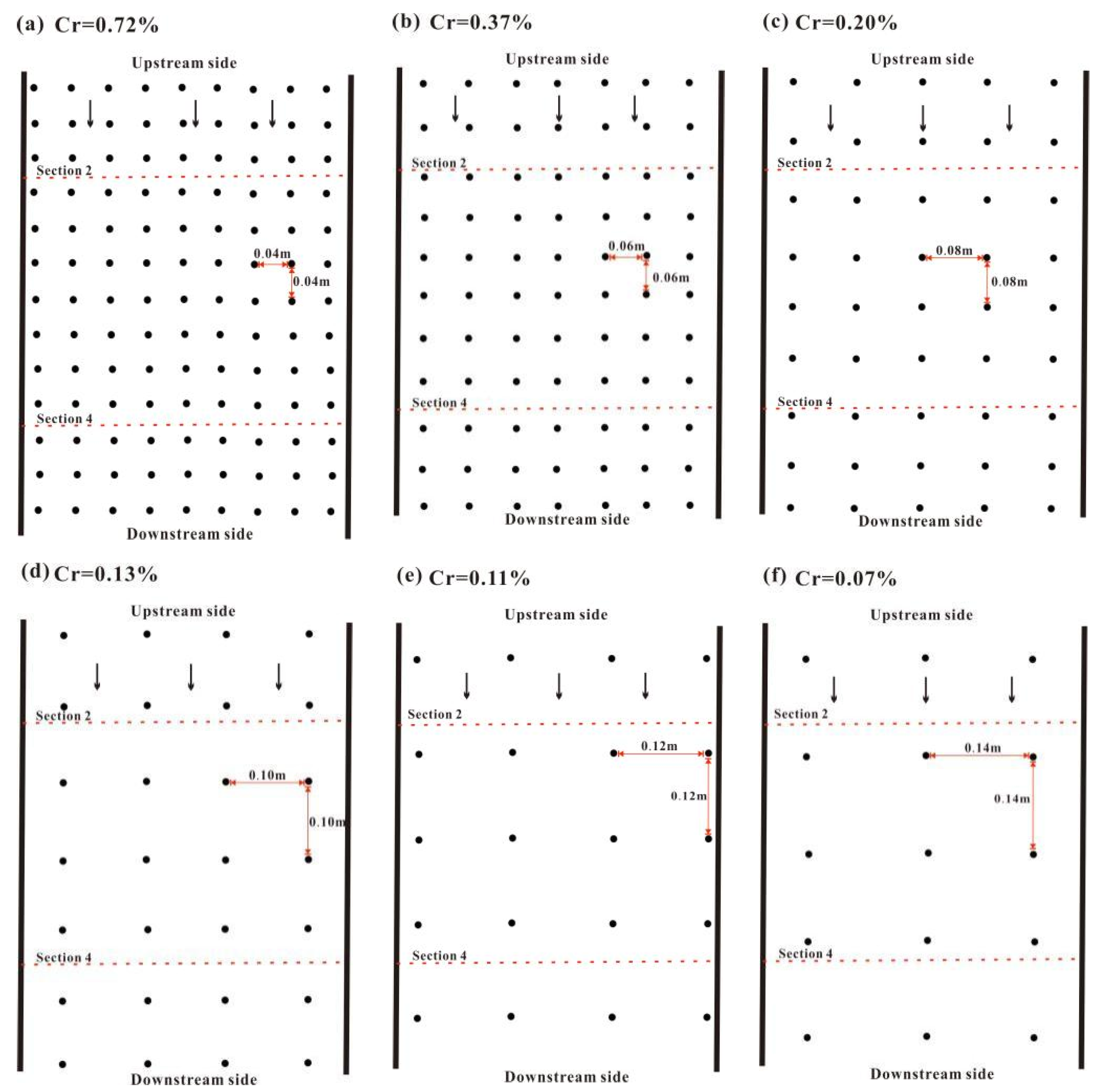
2.1. Experimental Structure

The overland flow study reported here mainly used the basic theory of flow in an open channel [57,58]. Many studies on the effects of vegetation on a slope during water erosion have used variable slopes involving rectangular flume experiments. To enhance the experimental effect and improve the experimental efficiency, single-plant vegetation has sometimes been generalized into an effective water-blocking cylinder in these experiments [59,60]. The structure of the test tank used in the present study is shown in Figure 1. The following design points were determined based on the purpose of the test:

(1) The test area was a polymethyl methacrylate flume. Four slopes (0, 1.0%, 2.0%, and 3.0%) were selected. The test flume was 5.0 m long with a width of 0.4 m and a height of 0.3 m; this flume was divided into three parts: an upstream flat water section (1 m), a vegetation coverage section (3 m), and a downstream water measuring section (1 m).

(2) Plastic cylindrical rods were used to simulate the stems of rigid vegetation. The height of the simulated vegetation (hv) was set at 0.15 m with a stem diameter (d) of 0.004 m to match the scale of the model. Simulated vegetation was arranged in a regular pattern; the distances between two rows of cylinders were 0.04 m, 0.06 m, 0.08 m, 0.10 m, 0.12 m, and 0.14 m, respectively. The ratios of stem diameter to adjacent plant spacing (d/l) were 10.00%, 6.67%, 5.00%, 4.00%, 3.33%, and 2.86%, respectively. The total number of cylindrical rods in each entire vegetation segment was 688, 420, 344, 239, 172, and 134, respectively. The stem cover (Cr) values assessed in this study were approximately 0.72%, 0.37%, 0.20%, 0.13%, 0.11%, and 0.07%, respectively (Figure 2), the corresponding stem cover (Cr) values can be calculated by using Equation (1) in the “Data Analysis” section.

(3) A quantitative analysis of the Manning roughness coefficient and hydraulic parameters was conducted to systematically study the effects of the change of stem vegetation on the internal relationship between the coefficient and parameters. The final design of seven discharge flows (Q) were 0.0313 m³/min, 0.1205 m³/min, 0.2190 m³/min, 0.3019 m³/min, 0.4241 m³/min, 0.5203 m³/min, and 0.6319 m³/min (0.0005 m³/s, 0.0020 m³/s, 0.0037 m³/s, 0.0050 m³/s, 0.0071 m³/s, 0.0087 m³/s, 0.0105 m³/s). In this study, a total of 168 water discharge tests were conducted, and 1176 sets of test data were obtained.

(4) In order to avoid the phenomenon of a high level of water jump in the upstream of the vegetation section and the downstream wake depth of the vegetation section, the influence of the flow instability on the test results was eliminated as much as possible. A water leveling device was set up upstream of the vegetation section, and observations of the length of the water depth and high area were performed downstream. Because the length of the upstream flat water section and the downstream water measuring section are both 1 m, it was found through observation that the upstream water jump and the downstream water flooding phenomenon did not affect the vegetation section. The length of the vegetation coverage section was 3 m, and 5 fixed longitudinal observation sections were set at equal intervals (As shown in Figure 1). The distance between adjacent sections is 0.75 m. In order to further ensure the full development of upstream water flows, this experiment used Section 2 and Section 4 as the observation sections for water depth measurement. The vegetation cover observation length was 1.5 m. As a result, the influence of the instability of the upstream water flow on the accuracy of the observation data of the vegetation section was further reduced.

2.2. Data Analysis

The ratio of the total area of stem vegetation to the total area of the flume bed of the vegetation test section is used to quantify the vegetative stem cover. Its expression is as follows:

$$Cr=\frac{N\pi d^2}{4WL}$$

(1)

where Cr is effective vegetative stem coverage (%), d is the diameter of the stem vegetation (m). N is the number of stem vegetation with diameter d. W is the width of the test flume (0.4 m), and L is the vegetation paving test section (3 m).

Because of the existence of stem vegetation, the cross-sectional area of overland flow is reduced; thus, the flume width cannot represent the effective flow width. The effective flow width is calculated as follows [61]:

$$w=W\times (1-Cr)$$

(2)

where w is the effective flow width of the section (m). The hydraulic radius R is the ratio of the interface water area to the wet circumference (m). It is expressed as follows:

$$R=A/P$$

(3)

P is the wet perimeter (m). A is the effective cross-sectional area of the flow (m²); it is expressed as follows:

$$A=w\times h$$

(4)

$$P=\frac{2hL+\left(WL-\frac{N\pi d^2}{4}\right)+N\pi dh}{L}$$

(5)

where h is the mean flow depth (m). The mean inter-stem velocity was estimated as follows:

$$V=Q/\left(w\times h\right)$$

(6)

where V is the mean velocity (m s⁻¹). Q is the discharge (m³ s⁻¹), which is determined by the electromagnetic flowmeter (Model: LDG—MIK—DN100).

During the experiment, we measured the pressure with piezometer tubes in Section 2 and Section 4 and recorded the flow depths as h₂ and h₄, respectively. R₂, R₄ and V₂, V₄ are respectively calculated by Equations (3) and (6). The flow depth h, current velocity V, and the hydraulic radius R were calculated using the mean values of cross Section 2 and Section 4 (i.e., h = (h₂ + h₄)/2; R = (R₂ + R₄)/2; V= (V₂ + V₄)/2).

The flow pattern is the basic parameter of the hydrodynamic characteristics. Generally, the Re and Fr are used to distinguish the flow pattern parameters. The Reynolds number is a parameter that reflects the motion state of a liquid and measures the ratio of inertial force to viscous force in the process of liquid flow. The Reynolds number can be expressed as

$$Re=\frac{VR}{\nu }$$

(7)

where R is the hydraulic radius, and $\nu$ is the motion viscosity coefficient (m²/s). Using the Poiseuille formula, $\nu$ was calculated as:

$$\nu =0.01775/\left(1+0.337T+0.00022T^2\right)$$

(8)

where $T$ is the temperature of the water (°C).

In the mechanical sense, the Froude number represents the ratio between the action of the inertial force and the action of gravity in the flow process of water. The expression of the Froude number is

$$Fr=\frac{V}{\sqrt{gh}}$$

(9)

where g is the acceleration due to gravity (m/s²).

Manning roughness coefficient, n, reflects the retardation effect of bed roughness on the flow process. The flow resistance of a vegetation slope is generally believed to mainly consist of boundary resistance or particle resistance and additional resistance caused by water flowing through vegetation, which can be obtained by Equation (10).

$$n=R^{2/3}{J}^{1/2}/V$$

(10)

where J is the hydraulic gradient.

The hydraulic gradient is the head loss per unit distance along the water flow path, which can be obtained by Equation (11).

$$J=\frac{h_f}{l}$$

(11)

where l is the length of water along the course (m). In this experiment, l is the distance between Section 2 and Section 4, with a length of 1.5 m. h_f is the frictional head loss (m)

$$h_f=\left(z_2-z_4\right)+\frac{(V_2^2-V_4^2)}{2g}$$

(12)

where $z_2$ and $z_4$ are the head height of the initial (Section 2) and final positions (Section 4) (m), and $\frac{(V_2^2-V_4^2)}{2g}$ is the flow head difference between the initial and final positions.

The following statistical parameters and equations were used to evaluate the performance of the Manning roughness coefficient. The Nash-Sutcliffe model efficiency (NSE) was calculated as

$$NSE=\frac{{{\displaystyle \sum }}_{i=1}^N{\left(O_i-O_{av}\right)}^2-{{\displaystyle \sum }}_{i=1}^N{\left(p_i-O_i\right)}^2}{{{\displaystyle \sum }}_{i=1}^N{\left(O_i-O_{av}\right)}^2}$$

(13)

where O_i, P_i, and O_av are the measured, analogue, and average values of the measured values, respectively, and N is the number of samples. Values of NSE closer to 1 indicate a better simulation effect of the model.

Through the calculation of the above formulas, the values of relevant hydraulic parameters under different stem cover conditions in four gentle slope states were obtained, which were used to systematically study the relationship between the slope flow resistance and water depth, flow pattern, stem density, and slope. The specific experimental data are shown in

Table 1. Experimental data of hydraulic parameters of six different vegetation stem cover under the condition of S = 0.0% (Cr is 0.72%, 0.37%, 0.20%, 0.13%, 0.11% and 0.07%, respectively).

Slope S (%)	Stem Cover Cr (%)	Q (m3/min)	Parameter
			Water Depth of the Measure Section		haverage (m)	Re	Fr	n
			h2 (m)	h4 (m)
0.0%	0.72%	0.0313	0.0148	0.0119	0.0134	1218	0.2756	0.0215
		0.1205	0.0351	0.0311	0.0331	3847	0.2692	0.0266
		0.2190	0.0536	0.0485	0.0511	6041	0.2552	0.0311
		0.3019	0.0660	0.0601	0.0630	7634	0.2562	0.0325
		0.4241	0.0832	0.0759	0.0796	9626	0.2540	0.0354
		0.5203	0.0961	0.0879	0.0920	10,962	0.2505	0.0371
		0.6319	0.1081	0.0990	0.1036	12,483	0.2547	0.0375
	0.37%	0.0313	0.0125	0.0102	0.0113	1254	0.3511	0.0147
		0.1205	0.0320	0.0296	0.0308	4145	0.2982	0.0197
		0.2190	0.0479	0.0450	0.0464	6803	0.2930	0.0221
		0.3019	0.0609	0.0575	0.0592	8687	0.2803	0.0247
		0.4241	0.0759	0.0716	0.0738	11,264	0.2833	0.0272
		0.5203	0.0875	0.0826	0.0850	13,039	0.2807	0.0286
		0.6319	0.1000	0.0947	0.0974	14,916	0.2783	0.0294
	0.20%	0.0313	0.0116	0.0262	0.0189	1458	0.1894	0.0187
		0.1205	0.0250	0.0381	0.0316	4664	0.2999	0.0234
		0.2190	0.0401	0.0527	0.0464	7641	0.2980	0.0254
		0.3019	0.0522	0.0646	0.0584	9841	0.2887	0.0267
		0.4241	0.0686	0.0804	0.0745	12,752	0.2805	0.0290
		0.5203	0.0798	0.0915	0.0856	14,862	0.2787	0.0292
		0.6319	0.0919	0.1030	0.0975	17,141	0.2782	0.0306
	0.13%	0.0313	0.0125	0.0112	0.0119	1330	0.3246	0.0126
		0.1205	0.0305	0.0290	0.0297	4619	0.3137	0.0149
		0.2190	0.0473	0.0450	0.0462	7723	0.2949	0.0201
		0.3019	0.0586	0.0557	0.0571	10,103	0.2952	0.0230
		0.4241	0.0744	0.0715	0.0730	13,220	0.2873	0.0235
		0.5203	0.0861	0.0825	0.0843	15,463	0.2839	0.0263
		0.6319	0.0975	0.0931	0.0953	17,967	0.2868	0.0287
	0.11%	0.0313	0.0137	0.0128	0.0133	5106	0.2736	0.0125
		0.1205	0.0334	0.0323	0.0328	17,976	0.2704	0.0156
		0.2190	0.0490	0.0478	0.0484	30,625	0.2745	0.0165
		0.3019	0.0603	0.0591	0.0597	40,371	0.2762	0.0159
		0.4241	0.0755	0.0739	0.0747	53,611	0.2770	0.0187
		0.5203	0.0869	0.0857	0.0863	63,102	0.2736	0.0160
		0.6319	0.0988	0.0968	0.0978	73,698	0.2757	0.0202
	0.07%	0.0313	0.0105	0.0079	0.0092	1286	0.4814	0.0106
		0.1205	0.0302	0.0285	0.0294	4382	0.3191	0.0159
		0.2190	0.0458	0.0443	0.0451	7396	0.3053	0.0164
		0.3019	0.0577	0.0560	0.0568	9676	0.2970	0.0181
		0.4241	0.0729	0.0714	0.0721	12,753	0.2919	0.0170
		0.5203	0.0840	0.0822	0.0831	14,980	0.2894	0.0185
		0.6319	0.0955	0.0941	0.0948	17,407	0.2885	0.0162

,

Table 2. Experimental data of hydraulic parameters of six different vegetation stem cover under the condition of S = 1.0% (Cr is 0.72%, 0.37%, 0.20%, 0.13%, 0.11% and 0.07%, respectively).

Slope S (%)	Stem Cover Cr (%)	Q (m3/min)	Parameter
			Water Depth of the Measure Section		haverage (m)	Re	Fr	n
			h2 (m)	h4 (m)
1.0%	0.72%	0.0313	0.0071	0.0064	0.0068	1297	0.7529	0.0176
		0.1205	0.0181	0.0223	0.0202	4360	0.5676	0.0227
		0.2190	0.0318	0.0387	0.0353	6897	0.4478	0.0254
		0.3019	0.0437	0.0497	0.0467	8622	0.4031	0.0285
		0.4241	0.0602	0.0642	0.0622	10,778	0.3668	0.0328
		0.5203	0.0734	0.0760	0.0747	12,160	0.3417	0.0361
		0.6319	0.0850	0.0878	0.0864	13,743	0.3339	0.0358
	0.37%	0.0313	0.0050	0.0045	0.0047	1376	1.2956	0.0097
		0.1205	0.0136	0.0154	0.0145	4898	0.9263	0.0155
		0.2190	0.0216	0.0310	0.0263	8360	0.7107	0.0176
		0.3019	0.0322	0.0433	0.0377	10,554	0.5626	0.0189
		0.4241	0.0482	0.0579	0.0530	13,323	0.4680	0.0228
		0.5203	0.0601	0.0687	0.0644	15,264	0.4277	0.0255
		0.6319	0.0722	0.0802	0.0762	17,372	0.4029	0.0272
	0.20%	0.0313	0.0109	0.0078	0.0094	1342	0.4751	0.0117
		0.1205	0.0318	0.0298	0.0308	4417	0.2985	0.0183
		0.2190	0.0480	0.0459	0.0469	7342	0.2882	0.0197
		0.3019	0.0599	0.0575	0.0587	9526	0.2838	0.0212
		0.4241	0.0725	0.0693	0.0709	12,621	0.3004	0.0232
		0.5203	0.0877	0.0844	0.0860	14,455	0.2754	0.0251
		0.6319	0.0997	0.0960	0.0979	16,692	0.2757	0.0265
	0.13%	0.0313	0.0038	0.0061	0.0049	1457	1.2748	0.0105
		0.1205	0.0132	0.0138	0.0135	5054	1.0237	0.0144
		0.2190	0.0205	0.0343	0.0274	8996	0.6878	0.0163
		0.3019	0.0318	0.0437	0.0377	11,335	0.5640	0.0191
		0.4241	0.0479	0.0600	0.0539	14,549	0.4578	0.0210
		0.5203	0.0604	0.0723	0.0664	16,797	0.4095	0.0225
		0.6319	0.0713	0.0823	0.0768	19,452	0.3985	0.0246
	0.11%	0.0313	0.0038	0.0051	0.0044	1356	1.4426	0.0092
		0.1205	0.0110	0.0130	0.0120	4909	1.2245	0.0123
		0.2190	0.0176	0.0298	0.0237	8839	0.8582	0.0160
		0.3019	0.0222	0.0420	0.0321	11,973	0.7746	0.0139
		0.4241	0.0413	0.0581	0.0497	14,481	0.5251	0.0133
		0.5203	0.0534	0.0687	0.0611	16,684	0.4669	0.0154
		0.6319	0.0662	0.0810	0.0736	19,110	0.4267	0.0163
	0.07%	0.0313	0.0048	0.0060	0.0054	1303	1.0671	0.0123
		0.1205	0.0124	0.0184	0.0154	4868	0.8715	0.0163
		0.2190	0.0168	0.0339	0.0253	9052	0.8173	0.0150
		0.3019	0.0208	0.0450	0.0329	12,247	0.7793	0.0122
		0.4241	0.0445	0.0605	0.0525	14,118	0.4808	0.0142
		0.5203	0.0562	0.0713	0.0638	16,374	0.4368	0.0160
		0.6319	0.0683	0.0832	0.0757	18,872	0.4081	0.0163

,

Table 3. Experimental data of hydraulic parameters of six different vegetation stem cover under the condition of S = 2.0% (Cr is 0.72%, 0.37%, 0.20%, 0.13%, 0.11% and 0.07%, respectively).

Slope S (%)	Stem Cover Cr (%)	Q (m3/min)	Parameter
			Water Depth of the Measure Section		haverage (m)	Re	Fr	n
			h2 (m)	h4 (m)
2.0%	0.72%	0.0313	0.0062	0.0032	0.0047	1475	1.4638	0.0114
		0.1205	0.0127	0.0145	0.0136	4637	1.0204	0.0195
		0.2190	0.0209	0.0241	0.0225	7714	0.8731	0.0230
		0.3019	0.0285	0.0364	0.0325	9779	0.7019	0.0269
		0.4241	0.0411	0.0526	0.0468	12,201	0.5698	0.0301
		0.5203	0.0517	0.0640	0.0578	13,746	0.5073	0.0321
		0.6319	0.0644	0.0764	0.0704	15,269	0.4570	0.0344
	0.37%	0.0313	0.0026	0.0039	0.0033	1447	2.3332	0.0080
		0.1205	0.0105	0.0115	0.0110	5024	1.4012	0.0145
		0.2190	0.0154	0.0192	0.0173	8774	1.3014	0.0167
		0.3019	0.0218	0.0245	0.0231	11,498	1.1527	0.0187
		0.4241	0.0267	0.0447	0.0357	15,588	0.8989	0.0224
		0.5203	0.0350	0.0583	0.0466	17,774	0.7367	0.0232
		0.6319	0.0425	0.0683	0.0554	20,319	0.6853	0.0228
	0.20%	0.0313	0.0022	0.0042	0.0032	1522	2.5853	0.0078
		0.1205	0.0114	0.0107	0.0110	4983	1.3902	0.0144
		0.2190	0.0179	0.0185	0.0182	8650	1.1918	0.0179
		0.3019	0.0198	0.0257	0.0227	11,769	1.1987	0.0188
		0.4241	0.0252	0.0466	0.0359	16,326	0.9156	0.0226
		0.5203	0.0302	0.0582	0.0442	19,304	0.8319	0.0224
		0.6319	0.0345	0.0701	0.0523	22,758	0.7992	0.0207
	0.13%	0.0313	0.0042	0.0032	0.0037	1416	1.8839	0.0089
		0.1205	0.0097	0.0116	0.0107	5176	1.4743	0.0142
		0.2190	0.0154	0.0169	0.0161	9061	1.4273	0.0152
		0.3019	0.0195	0.0221	0.0208	12,184	1.3474	0.0167
		0.4241	0.0210	0.0381	0.0295	17,558	1.2180	0.0206
		0.5203	0.0284	0.0525	0.0404	20,401	0.9368	0.0227
		0.6319	0.0332	0.0617	0.0475	23,928	0.8961	0.0226
	0.11%	0.0313	0.0042	0.0047	0.0044	1330	1.4198	0.0127
		0.1205	0.0107	0.0106	0.0107	4916	1.4591	0.0139
		0.2190	0.0154	0.0148	0.0151	8717	1.5694	0.0132
		0.3019	0.0195	0.0172	0.0184	11,838	1.6228	0.0124
		0.4241	0.0250	0.0361	0.0305	15,999	1.0961	0.0212
		0.5203	0.0284	0.0487	0.0386	19,462	0.9845	0.0227
		0.6319	0.0332	0.0605	0.0469	22,991	0.9078	0.0228
	0.07%	0.0313	0.0038	0.0045	0.0042	1305	1.5701	0.0115
		0.1205	0.0103	0.0102	0.0103	4829	1.5414	0.0131
		0.2190	0.0148	0.0160	0.0154	8554	1.5287	0.0143
		0.3019	0.0182	0.0202	0.0192	11,574	1.5183	0.0149
		0.4241	0.0235	0.0381	0.0308	16,096	1.1061	0.0214
		0.5203	0.0268	0.0520	0.0394	19,772	0.9872	0.0227
		0.6319	0.0302	0.0620	0.0461	23,620	0.9655	0.0227

and

Table 4. Experimental data of hydraulic parameters of six different vegetation stem cover under the condition of S = 3.0% (Cr is 0.72%, 0.37%, 0.20%, 0.13%, 0.11% and 0.07%, respectively).

Slope S (%)	Stem Cover Cr (%)	Q (m3/min)	Parameter
			Water Depth of the Measure Section		haverage (m)	Re	Fr	n
			h2 (m)	h4 (m)
3.0%	0.72%	0.0313	0.0059	0.0021	0.0040	1733	2.1338	0.0083
		0.1205	0.0136	0.0094	0.0115	4980	1.3546	0.0170
		0.2190	0.0202	0.0177	0.0189	8167	1.1312	0.0217
		0.3019	0.0261	0.0246	0.0253	10,553	1.0050	0.0248
		0.4241	0.0338	0.0389	0.0363	13,485	0.8250	0.0295
		0.5203	0.0403	0.0547	0.0475	15,326	0.6898	0.0322
		0.6319	0.0483	0.0657	0.0570	17,344	0.6380	0.0329
	0.37%	0.0313	0.0035	0.0022	0.0029	1471	2.9053	0.0062
		0.1205	0.0098	0.0088	0.0093	5097	1.7923	0.0131
		0.2190	0.0152	0.0145	0.0148	8851	1.6196	0.0154
		0.3019	0.0189	0.0181	0.0185	11,866	1.6071	0.0157
		0.4241	0.0248	0.0247	0.0248	15,916	1.4560	0.0179
		0.5203	0.0291	0.0292	0.0292	18,926	1.3955	0.0189
		0.6319	0.0311	0.0371	0.0341	22,372	1.3525	0.0206
	0.20%	0.0313	0.0034	0.0017	0.0026	1534	3.6021	0.0041
		0.1205	0.0091	0.0086	0.0088	5055	1.9421	0.0122
		0.2190	0.0159	0.0140	0.0149	8859	1.6079	0.0154
		0.3019	0.0204	0.0180	0.0192	11,885	1.5234	0.0166
		0.4241	0.0242	0.0238	0.0240	16,162	1.5243	0.0174
		0.5203	0.0280	0.0279	0.0279	19,369	1.4884	0.0181
		0.6319	0.0324	0.0324	0.0324	22,929	1.4490	0.0187
	0.13%	0.0313	0.0032	0.0021	0.0026	1460	3.1964	0.0056
		0.1205	0.0086	0.0097	0.0092	5198	1.8405	0.0135
		0.2190	0.0132	0.0146	0.0139	9187	1.7905	0.0148
		0.3019	0.0164	0.0176	0.0170	12,417	1.8144	0.0148
		0.4241	0.0204	0.0232	0.0218	17,027	1.7675	0.0161
		0.5203	0.0255	0.0293	0.0274	20,274	1.5401	0.0187
		0.6319	0.0287	0.0375	0.0331	24,155	1.4269	0.0211
	0.11%	0.0313	0.0031	0.0033	0.0032	1336	2.3287	0.0090
		0.1205	0.0090	0.0072	0.0081	5048	2.2281	0.0098
		0.2190	0.0137	0.0107	0.0122	8992	2.2080	0.0098
		0.3019	0.0161	0.0145	0.0153	12,029	2.1365	0.0113
		0.4241	0.0194	0.0186	0.0190	16,522	2.1598	0.0118
		0.5203	0.0235	0.0210	0.0222	19,966	2.1012	0.0115
		0.6319	0.0271	0.0249	0.0260	23,738	2.0127	0.0125
	0.07%	0.0313	0.0033	0.0048	0.0040	1344	1.6988	0.0131
		0.1205	0.0095	0.0076	0.0086	4932	2.0548	0.0109
		0.2190	0.0145	0.0121	0.0133	8701	1.9099	0.0124
		0.3019	0.0178	0.0156	0.0167	11,741	1.8746	0.0131
		0.4241	0.0238	0.0223	0.0230	15,920	1.6200	0.0162
		0.5203	0.0268	0.0278	0.0273	19,103	1.5359	0.0182
		0.6319	0.0295	0.0331	0.0313	22,817	1.5259	0.0191

.

3. Results and Discussion

3.1. Statistical Analysis

All statistical analyses were performed in First Optimization software (version 5.0). To analyze the correlations between the resistance coefficient and hydraulic parameters, gravel coverage degrees, slope gradients, and flow discharges, a regression analysis was implemented to quantify the relationship between independent and dependent variables.

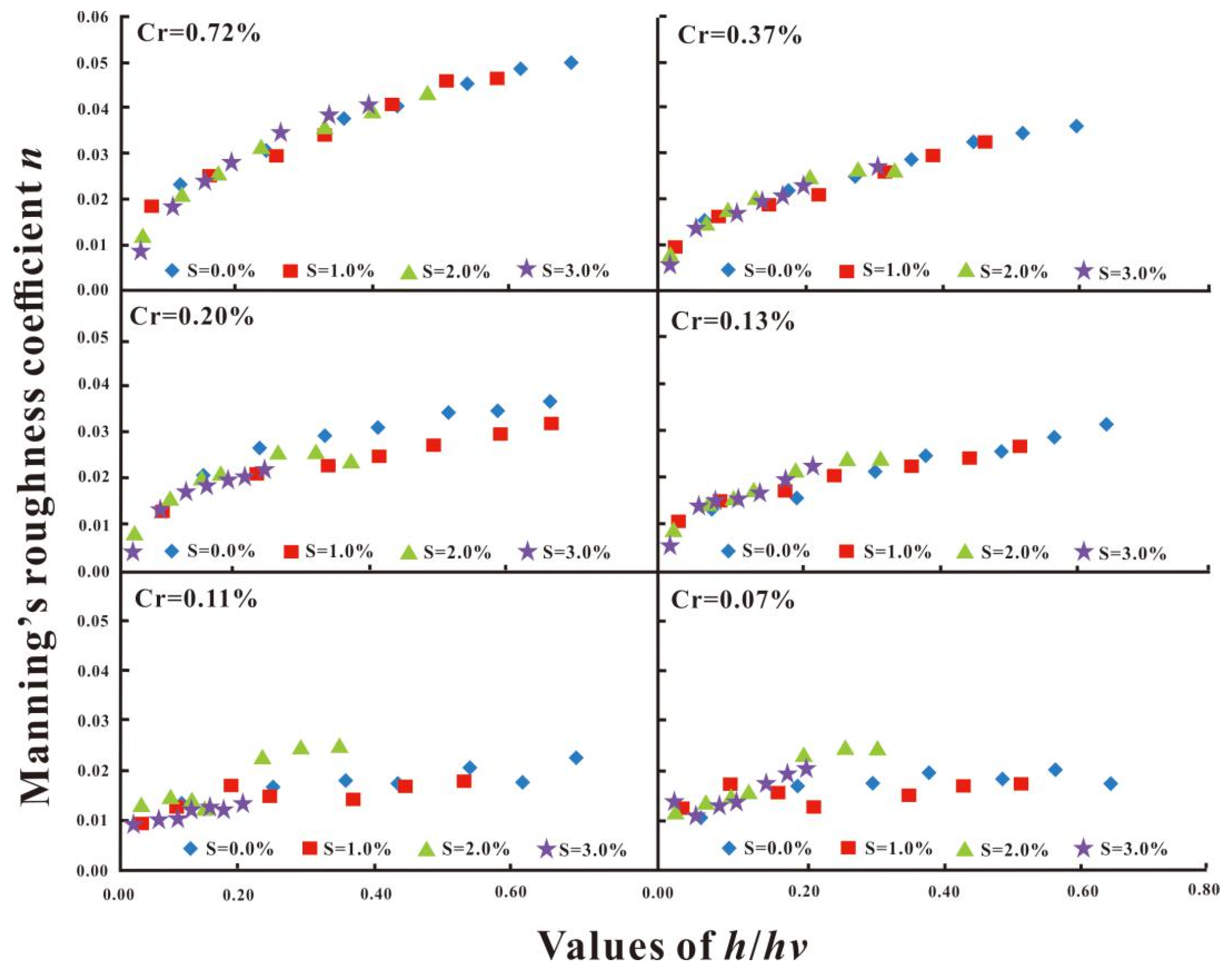
3.2. The Relationship between n and h/hv under Different Density and Slope Conditions

It is generally believed that the resistance caused by vegetation to water flow acts on the water body along the water depth [62,63]; then, the flow resistance coefficient is positively related to the water depth. It should be pointed out that this experiment is related to the non-submerged state of vegetation. In order to make the experiment and the results show better physical meaning, this study did not directly choose the water depth but the ratio h/hv of the water depth to the height of the vegetation, and the study was carried out in a dimensionless form. Variation characteristics of water flow resistance coefficient under different coverage density and slope conditions. In order to further analyze the variation law of the flow resistance coefficient for overland flow with non-submerged vegetation, the test data were organized as shown in Figure 3.

Figure 3 shows the trend of variation in the vegetation Manning roughness coefficient n with the values of h/hv under six coverage conditions. Under six different stem cover densities, n increased with h/hv as a power function (Figure 3). This is consistent with the conclusion that the relationship between flow resistance and water depth in Zhang et al. [64] and Juha [65] was based on the influence of the distribution of vegetation on slope flow resistance. In terms of the coefficient of resistance and values of h/hv, as the vegetation coverage increased, the correlation between the coefficient of resistance and values of h/hv strengthened, which is consistent with the results of previous literature [66,67]. When Cr ≥ 0.13%, its regression correlation coefficient R² was always greater than 0.8835 (mean was approximately 0.9266); when Cr ≤ 0.11%, the correlation between the resistance coefficient and h/hv was weak, and its regression correlation coefficient R² was less than 0.5769 (mean was approximately 0.5109). In addition, the n value of all test points did not increase from zero, which was caused by the wall friction from the plexiglass plate laid on the test floor; Jin et al. [25] and Jeon et al. [68] also had similar ideas related to the flow resistance of partially submerged stems.

The dn/d (h/hv) ratio increased with increasing vegetation coverage (Figure 3). This indicates that under high coverage, when Re is held constant and the increase in velocity is small, the water depth is bound to increase which causes the drag caused by vegetation in increase along the water depth. The drag caused by the wall friction was far less than the additional resistance of the vegetation. This is consistent with the conclusion of James et al. [69] on the additional resistance of vegetation. In addition, with a constant values of h/hv, the coverage and the resistance coefficient were positively correlated. Under the same coverage, the slope has almost no effect on the resistance coefficient.

The factors affecting resistance to overland flow in areas covered by vegetation mainly include ratio of water depth to vegetation height, coverage, slope, flow, and so on. The power function formula between h/hv, Cr, S and n can be obtained using data regression analysis. The NSE values in Equations (14) and (15) were 0.8571 and 0.8528, respectively, which are close to 1, indicating that the equation is very good. The absolute value of the index of each variable can reflect the sensitivity of the change to the resistance coefficient. It can be seen that under the condition of zero slope, Cr (0.2968) has a slightly greater influence on the drag coefficient than h/hv (0.2941), so it is the dominant factor affecting the overland flow resistance. Under the condition of non-zero slope, h/hv (0.3472) is the dominant factor affecting the resistance coefficient, followed by Cr (0.1986) and S (0.0873), the latter having the smallest effect.

$$n=0.1894C{r}^{0.2968}{\left(h/hv\right)}^{0.2941},NSE=0.8571,N=42,S=0$$

(14)

$$n=0.1621C{r}^{0.1968}{S}^{0.0873}{\left(h/hv\right)}^{0.3472},NSE=0.8528,N=126,S\ne 0$$

(15)

3.3. The Relationship between n and Re under Different Density and Slope Conditions

For the open channel flow of submerged vegetation, n is a constant, which does not change with a change in water depth, Reynolds number, and relative roughness, but is related to the boundary material. Due to the influence of surface conditions such as vegetation shape, stiffness, density, and distribution form, the relationship between n and Re of overland flow with vegetation is more complicated than that of open channel flow, and its change trend is closely related to the composition of rough vegetation units. Figure 4 plots the variation law of n and Re under different coverage, which can be used to explore the characteristics of vegetation resistance.

Figure 4 shows the range of the Re value was 1218–24,155; the research flow patterns were transition flow and turbulent flow. Under six coverage conditions, n increased with the increase of Re, which is consistent [11,70] or inconsistent [8,71,72,73] with the research conclusions of various scholars. This is true because the former group of scholars studied turbulent flow, while the latter group studied laminar, from which it can be inferred that the flow pattern of the overland flow is the main factor affecting the relationship between the resistance coefficient and Re. This phenomenon may occur because the composition of the flow resistance is different in different conditions. In the case where Re is very small, because the flow is not easily spread across the entire bottom slope, the boundary resistance generated by the inner wall of the flume has an absolute advantage over the morphological resistance due to the presence of vegetation; as Re increases, the boundary resistance is continuously decreasing while the morphological resistance is prominent.

When Cr is relatively large, the rate of change of n with Re is relatively large; that is, the larger Re is, the greater the increment of n is. This is true because an increase in vegetation density reduces the cross section of water area, increases the wet cycle of vegetation flow, and increases the solid-liquid contact area, so the vegetation change rate is greater. It can also be seen from Figure 4 that when Cr ≥ 0.13%, under the condition of the same coverage density and the same Reynolds number, a larger S corresponds to a smaller n value. When Cr decreases further ≤ 0.11%, this phenomenon gradually disappears.

The occurs because as the slope continues to increase, the potential energy of the flow and the inertial force of the flow both increased continuously; the turbulence of the flow also increased continuously, causing under the same Re conditions. The thickness of the water layer on the slope is lessened, the solid–liquid contact area is continuously reduced, the Manning roughness coefficient decreases, and the flow resistance capacity of slope decreases correspondingly. However, when the amount of vegetation coverage is relatively small, the influence of slope on the resistance coefficient is difficult to reflect because the morphological resistance of vegetation plays only a small role.

The power function formula between Re, Cr, S and n can be obtained based on the regression analysis data. Using Equations (16) and (17), the NSE values were 0.6944 and 0.7767, respectively, the representation effect of the model is relatively general. According to the fitting formula, Cr and Re are positively correlated with n, while S and n are negatively correlated with each other. Moreover, under zero slope condition, Cr (0.3283) is the dominant factor affecting the Manning roughness coefficient, under non-zero slope test condition, Re (0.3372) is the leading factor affecting the resistance coefficient, followed by Cr (0.2912) and finally S (0.2085).

$$n=0.0476C{r}^{0.3283}R{e}^{0.1393},NSE=0.6944,N=42,S=0$$

(16)

$$n=0.0021C{r}^{0.2912}{S}^{-0.2085}R{e}^{0.3372},NSE=0.7767,N=126,S\ne 0$$

(17)

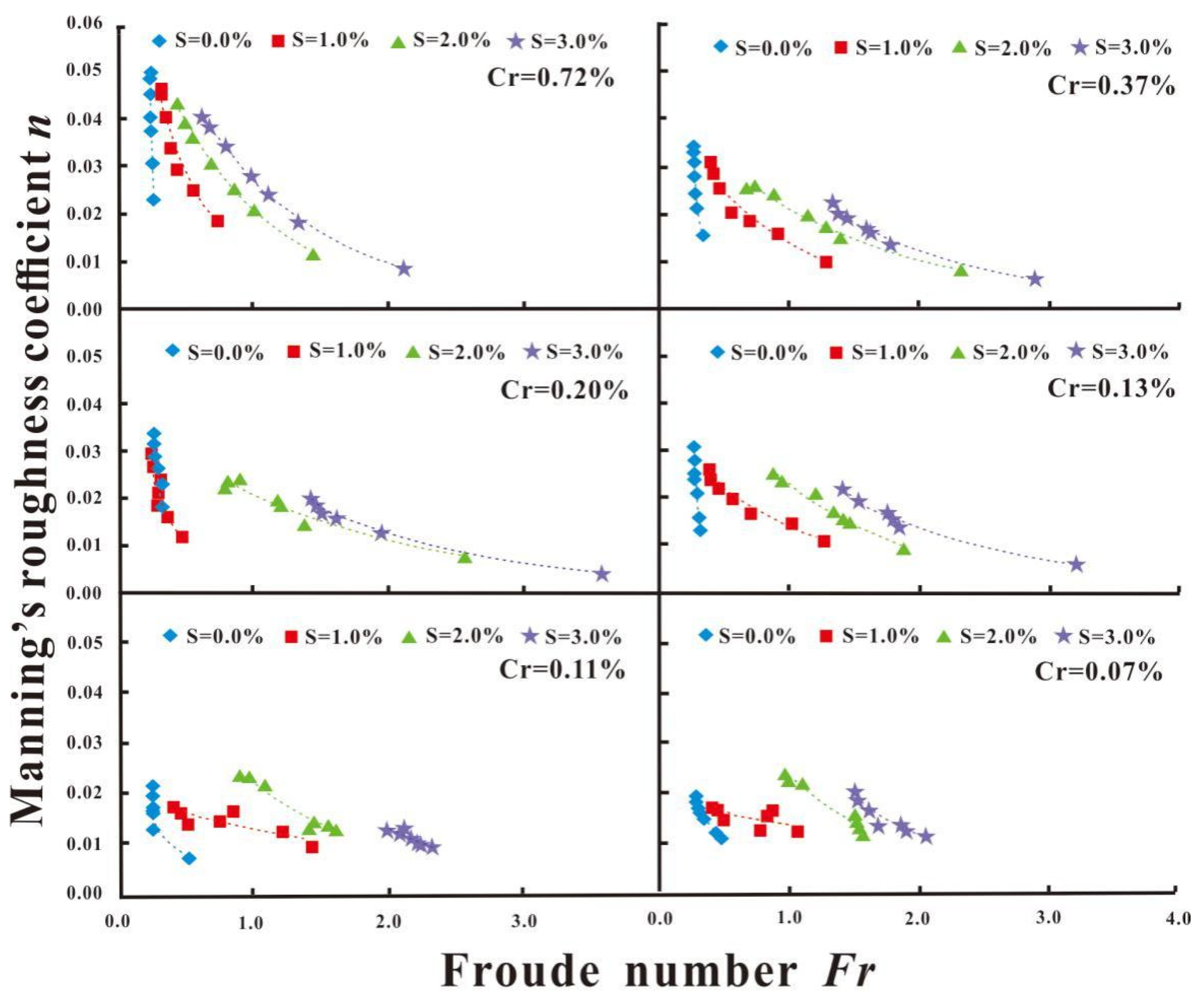
3.4. The Relationship between n and Fr under Different Density and Slope Conditions

The resistance coefficient is closely related to the Reynolds number, but also to its Froude number. The Fr is used to indicate whether the overland flow is in a rapid-flow or slow-flow state and represents the ratio of inertia force to gravity. When the flow rate is basically held unchanged, with a larger Froude number the average flow velocity of overland runoff will be larger, runoff will have a stronger ability to cause erosion, the water depth will be shallower, and the runoff on the slope will be smaller. Previous studies have considered that there is a power function relationship between the resistance coefficient and the Froude number, but the influence of coverage and slope has seldom been considered. In order to fully consider the relationship between the resistance coefficient and the Froude number under different coverage and slope conditions, the test data were organized as shown in Figure 5.

The Fr value ranged within 0.1894 and 3.6021 showing the flow pattern evolved from subcritical to supercritical flow (Figure 5). With an increase of Fr, n showed a decreasing trend, which is similar to the conclusions of Li et al. [70] and Zhang et al. [11]; Fr basically presents the change rule of a power function. When Fr is constant, a larger S resulted in a greater resistance coefficient. As coverage decreases, the correlation between n and Fr weaker, and the range of n values is shranking (Figure 5). Under the same coverage conditions, as the slope increased, the flow from slow to rapid development improved. In addition, when the slope S ≤ 1.0% the flow state under this study conditions was slow flow; meanwhile, when the slope S > 1.0% the flow changed to rapids flow.

Using the data regression analysis, the power function formula for Fr, Cr, S and n could be obtained. Compared with other hydraulic parameters, the correlation was slightly worse, and the NSE values in Equations (18) and (19) were 0.5587 and 0.7613, respectively. According to the fitting formula, under a constant Fr condition, Cr and S were positively correlated with n, while Fr and n were negatively correlated. In addition, within the slope range of this test, Fr was the leading factor affecting the resistance coefficient, followed by S and finally Cr.

$$n=0.0496C{r}^{0.2396}F{r}^{-0.5458},NSE=0.5587,N=42,S=0$$

(18)

$$n=0.2502C{r}^{0.1079}{S}^{0.4998}F{r}^{-0.6186},NSE=0.7613,N=126,S\ne 0$$

(19)

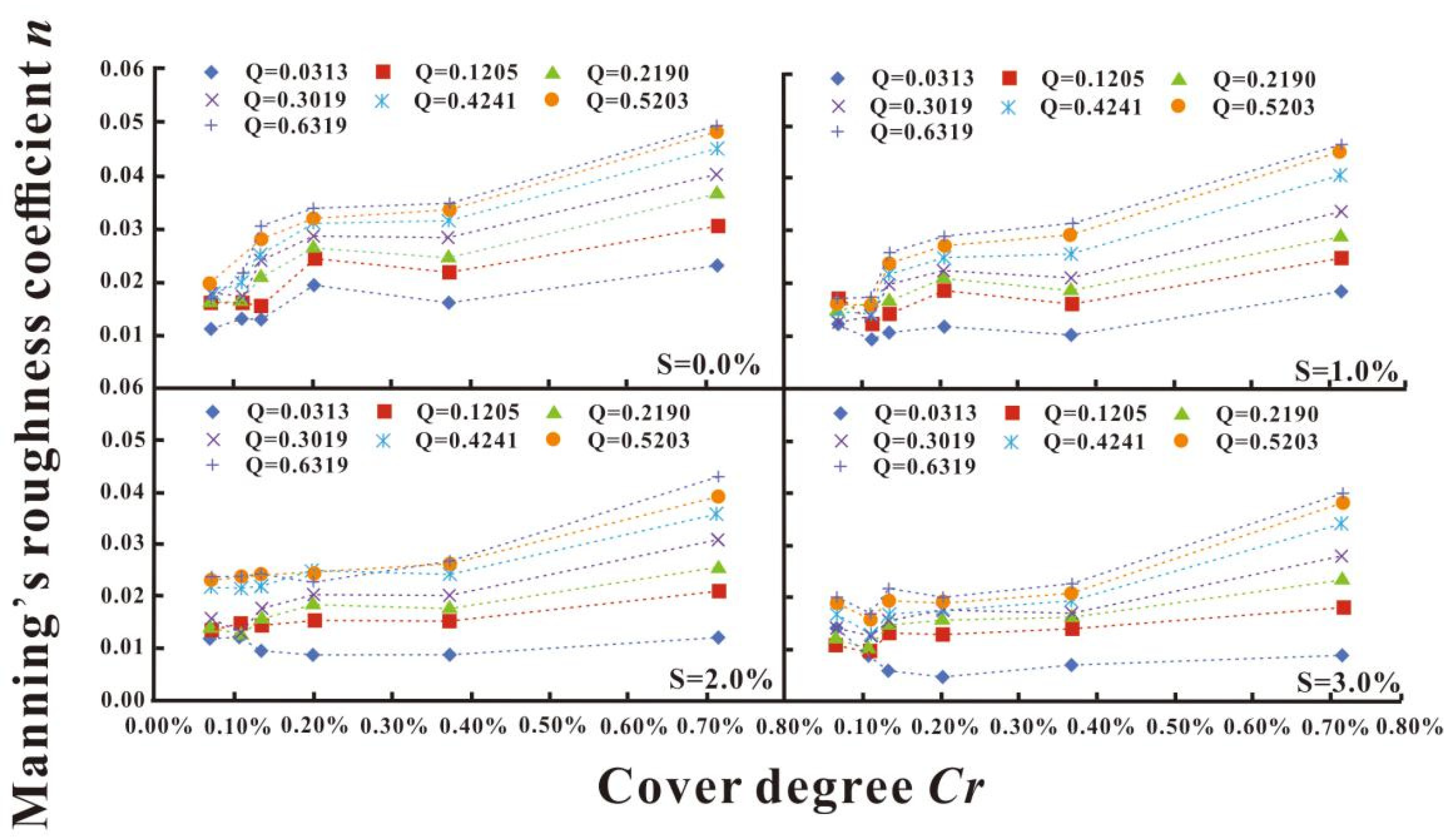
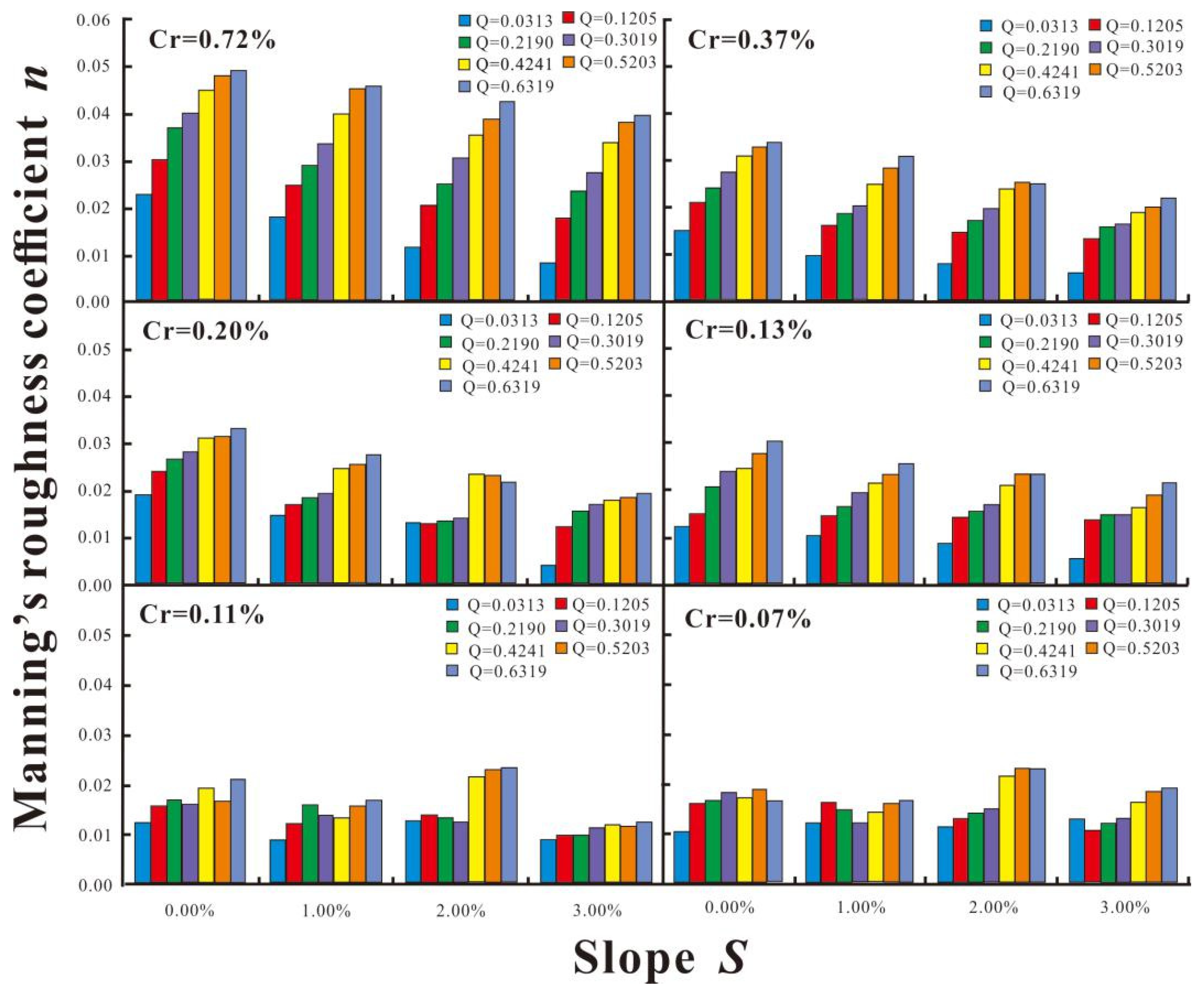
3.5. The Relationship between n and Cr and S under Different Flow Discharge Conditions

The density of vegetation coverage and the slope are important factors affecting the change of resistance of sloping surface. In order to further study the influence of coverage density and slope on the Manning roughness coefficient, the experimental data are organized as shown in Figure 6 and Figure 7. Under the four slope conditions, n gradually increased with an increase of Cr, and dn/dCr gradually decreased with an increase of slope, especially when the S is 2.0% or 3.0%; with Cr continuously increasing from 0.07% to 0.37%, n was basically in a steady change (Figure 6). In addition, under the same coverage conditions, n increased with an increase of Q and the two were positively correlated. This finding was consistent with some previous results showing that the Manning roughness coefficient increased with an increasing degree of coverage [19,33,34,35]. This occurred because under the same flow conditions with greater vegetation coverage the double-layer advantages of the number of plants and the thickness of the backwater increased the solid–liquid contact area, and the water blocking ability was bound to increase.

However, some inconsistent opinions have been expressed related to the relationship between the resistance coefficient and slope gradient. Wang et al. [74] study showed that under the steep slope test conditions where the flow regime is laminar flow, when the vegetation coverage is greater than 4.65%, the resistance coefficient decreases with the increase of the slope, that is, the two are in a negative correlation. When the vegetation coverage is less than 4.65%, the slope has little effect on resistance coefficient, and there is basically no change with the increase in slope. Pan and Shangguan [73,75] showed that under the condition of laminar flow steep slope, for bare slope, the surface water resistance coefficient increased with the increase of slope, while the slope vegetation coverage was 70%, showing an opposite trend. It can be seen that the vegetation coverage is an important factor affecting the trend change between the resistance coefficient and the slope. However, under the condition of gentle slope with transitional flow and turbulent flow, the influence of sparse stem vegetation coverage on the relationship between overland flow resistance coefficient and slope remains to be studied. In order to further explore the inherent relationship between the two, the test data is sorted out as shown in Figure 7.

When the stem coverage density was 0.72% to 0.13%, n decreased with an increase of S; that is, a negative correlation existed between n and S. As the coverage decreased further (Cr ≤ 0.11%), the slope had little effect on the roughness coefficient. This indicates that with the decrease of vegetation cover density to a certain extent, particle resistance plays a dominant role in water flow resistance, while vegetation form resistance plays a small role, which is similar to the conclusion of Zhang et al. [76] that “particle resistance is not or rarely affected by slope S”, so Manning roughness coefficient tends to be stable with the increase of slope.

Because Figure 6 and Figure 7 both reflect the relationship between Cr, S, and n under different flow discharges, the power function formula between Cr, S, Q, and n could be obtained based on the data regression analysis. In Equations (20) and (21), the NSE values were 0.8550 and 0.8095, respectively, and was close to 1 showing equation was optimal. According to the fitting formula, Cr, Q and n are positively correlated under the same flow condition, negative correlation existed between S and n. It can be seen that under the condition of zero slope, the influence of Cr (0.2693) on the flow resistance of slope is obviously greater than that of Q (0.1994), so it is the dominant factor affecting the overland flow resistance. Under the condition of non-zero slope, Q (0.2997) is the dominant factor affecting the resistance coefficient, followed by Cr (0.2540) and S (0.1529), the latter having smallest effect.

$$n=0.1562C{r}^{0.2693}{Q}^{0.1994},NSE=0.8550,N=42,S=0$$

(20)

$$n=0.0691C{r}^{0.2540}{S}^{-0.1529}F{r}^{0.2997},NSE=0.8095,N=126,S\ne 0$$

(21)

4. Conclusions

For overland flows with discharges ranging from 0.0313 to 0.6319 m³/min and a slope from 0% to 3.0%, a number of hydraulic parameters were measured with a vegetative stem cover from 0.07% to 0.72% to investigate the effects of the resistance to overland flow under the condition of sparse stem cover. The following conclusions can be drawn based on this experimental study:

The value of n showed a power function increasing with an increase of h/hv; the correlation between n and h/hv was stronger with an increase in vegetation cover. Meanwhile, dn/d (h/hv) increased with an increase of Cr. Under the condition of zero slope, Cr was the dominant factor affecting the overland flow resistance. Under the condition of non-zero slope, h/hv was the dominant factor affecting the resistance coefficient, followed by Cr and S, the latter having smallest effect.

In addition, n increased with an increase of Re; when Cr was greater, the rate of change of n with Re was larger. Also, Cr and Re were positively correlated with n. Under the same Fr both Cr and S were positively correlated with n, and Fr and n were negatively correlated with each other.

The value of n gradually increased with an increase of Cr; the dn/dCr ratio gradually decreased with an increase of S. Under the same Cr, n had a positive correlation with Q. Meanwhile, n decreased with increasing S, so the two had a negative correlation. As the coverage decreased further (Cr ≤ 0.11%), S had little effect on the roughness coefficient.

In short, the relationship between n and h/hv, Re, Cr, and S all shows the same law; that is, for sparse stem vegetation coverage, Cr is the dominant factor affecting overland flow resistance under zero slope condition, while Cr is no longer the first dominant factor affecting overland flow resistance under non-zero slope condition. Therefore, Cr is an important factor affecting slope flow resistance and hydraulic parameters.

References

1. Cheng, N.S.; Nguyen, H.T.; Tan, S.K.; Shao, S.D. Scaling of velocity profiles for depth-limited open channel flows over simulated rigid vegetation. J. Hydraul. Eng. 2012, 138, 673–683. [Google Scholar] [CrossRef]
2. Zhang, K.D.; Wang, G.Q.; Sun, X.M.; Wang, J.J. Hydraulic characteristic of overland flow under different vegetation coverage. Adv. Water Sci. 2014, 25, 825–834. [Google Scholar]
3. Vargas-Luna, A.; Crosato, A.; Uijttewaal, W.S.J. Effects of vegetation on flow and sediment transport: Comparative analyses and validation of predicting models. Earth Surf. Proc. Land. 2015, 40, 157–176. [Google Scholar] [CrossRef]
4. Zhu, H.C.; Zhao, Y.P.; Liu, H.Y. Scale characters analysis for gully structure in the watersheds of loess landforms based on digital elevation models. Front. Earth Sci. Pro. 2018, 12, 431–443. [Google Scholar] [CrossRef]
5. Dunkerley, D.L. Flow threads in surface runoff: Implications for the assessment of flow properties and friction coefficients in soil erosion and hydraulics investigations. Earth Surf. Proc. Land. 2004, 29, 1012–1026. [Google Scholar] [CrossRef]
6. Ali, M.; Sterk, G.; Seeger, M. Effect of flow discharge and median grain size on mean flow velocity under overland flow. J. Hydrol. 2012, 337, 150–160. [Google Scholar] [CrossRef]
7. Wang, W.J.; Huai, W.X.; Zeng, Y.H.; Zhou, J.F. Analytical solution of velocity distribution for flow through submerged large deflection flexible vegetation. Appl. Math. Mech. 2015, 36, 107–120. [Google Scholar] [CrossRef] [Green Version]
8. Ding, W.F.; Li, M. Effects of grass coverage and distribution patterns on erosion and overland flow hydraulic characteristics. Environ. Earth Sci. 2016, 75, 1–14. [Google Scholar] [CrossRef]
9. Mohammadiun, S.; Neyshabouri, S.A.A.S.; Naser, G.; Vahabi, H. Numerical investigation of submerged vane effects on flow pattern in a 90 junction of straight and bend open channels. Iran J. Sci. Technol. Trans. Civ. Eng. 2016, 40, 1–17. [Google Scholar] [CrossRef]
10. Yasi, M.; Ashori, M. Environmental flow contributions from inbasin rivers and dams for saving Urmia lake. Iran J. Sci. Technol. Trans. Civ. Eng. 2017, 41, 1–10. [Google Scholar] [CrossRef]
11. Zhang, S.T.; Zhang, J.Z.; Liu, Y.; Liu, Y.C. Effects of farmland vegetation row direction on overland flow hydraulic characteristics. Hydrol. Res. 2018, 49, 1991–2001. [Google Scholar] [CrossRef] [Green Version]
12. Zhou, Z.; Li, X.; Chen, L.; Li, B.; Liu, T. Macrobenthic assemblage characteristics under stressed waters and ecological health assessment using AMBI and M-AMBI: A case study at the Xin’an River Estuary, Yantai, China. Acta Oceanol. Sin. 2018, 37, 77–86. [Google Scholar] [CrossRef]
13. Turner, A.K.; Chanmeesri, N. Shallow flow of water through non-submerged vegetation. Agric. Water Manag. 1984, 8, 375–385. [Google Scholar] [CrossRef]
14. Weltz, M.A.; Arsland, A.B.; Lane, L.J. Hydraulic roughness coefficients for native rangelands. J. Irrig. Drain. Eng. 1992, 118, 776–790. [Google Scholar] [CrossRef] [Green Version]
15. Gilley, J.E.; Kottwitz, E.R. Darcy-Weisbach roughness coefficients for selected crops. Trans. ASAE 1994, 37, 467–471. [Google Scholar] [CrossRef]
16. Wu, F.S. Characteristics of flow resistance in open channels with non-submerged rigid vegetation. J. Hydrodyn. Ser. B 2008, 20, 239–245. [Google Scholar] [CrossRef]
17. Cao, Y.; Zhang, G.; Tang, K.; Luo, R. Experiment on the effect of simulated surface cover on the overland flow velocity. J. Mt. Sci. 2011, 29, 654–659. [Google Scholar]
18. Fathi-Moghadam, M.; Drikvandi, K. Manning roughness coefficient for rivers and flood plains with non-submerged vegetation. Int. J. Hydraulic. Eng. 2012, 1, 1–4. [Google Scholar]
19. Zhao, C.; Gao, J.; Huang, Y.; Wang, G.; Zhang, M. Effects of vegetation stems on hydraulics of overland flow under varying water discharges. Land Degrad. Dev. 2016, 27, 748–757. [Google Scholar] [CrossRef]
20. Abrahams, A.D.; Parsons, A.J.; Wainwright, J. Resistance to overland flow on semiarid grassland and shrubland hillslopes, Walnut Gulch, southern Arizona. J. Hydrol. 1994, 156, 431–446. [Google Scholar] [CrossRef]
21. Järvelä, J. Effect of Submerged Flexible Vegetation on Flow Structure and Resistance. J. Hydrol. 2005, 307, 233–241. [Google Scholar] [CrossRef]
22. Gabarròn-Galeote, M.A.; Mart ınez-Murillo, J.F.; Quesada, M.A.; Ruiz-Sinoga, J.D. Seasonal Changes in the Soil Hydrological and Erosive Response Depending on Aspect, Vegetation Type and Soil Water Repellency in Different Mediterranean Micro Environments. Solid Earth 2013, 4, 497–509. [Google Scholar] [CrossRef] [Green Version]
23. Xia, J.H.; Nehal, L. Hydraulic features of flow through emergent bending aquatic vegetation in the riparian zone. Water 2013, 5, 2080–2093. [Google Scholar] [CrossRef]
24. Okamoto, T.A.; Nezu, I. Turbulence structure and “Monami” phenomena in flexible vegetated open-channel flows. J. Hydraul. Res. 2009, 47, 798–810. [Google Scholar] [CrossRef]
25. Jin, C.X.; Römkens, M.J.M.; Griffioen, F. Estimating Manning’s roughness coefficient for shallow overland flow in non-submerged vegetative filter strips. Trans. ASAE 2000, 43, 1459–1466. [Google Scholar] [CrossRef]
26. Kothyari, U.C.; Hayashi, K.; Hashimoto, H. Drag coefficient of unsubmerged rigid vegetation stems in open channel flows. J. Hydraul. Res. 2009, 48, 829–830. [Google Scholar] [CrossRef]
27. Kowobary, T.S.; Rice, C.E.; Garton, J.E. Effect of roughness elements on hydraulic resistance for overland flow. Trans. ASAE 1972, 15, 979–984. [Google Scholar] [CrossRef]
28. Carollo, F.G.; Ferro, V.; Termini, D. Flow resistance law in channels with flexible submerged vegetation. J. Hydraul. Eng. 2005, 131, 554–564. [Google Scholar] [CrossRef] [Green Version]
29. Ghisalberti, M.; Nepf, H.M. The structure of the shear layer in flows over rigid and flexible canopies. Environ. Fluid Mech. 2006, 6, 277–301. [Google Scholar] [CrossRef]
30. Nepf, H.M. Hydrodynamics of vegetated channels. J. Hydraul. Res. 2012, 50, 262–279. [Google Scholar] [CrossRef] [Green Version]
31. Ferro, V. Assessing flow resistance law in vegetated channels by dimensional analysis and self-similarity. Flow Meas. Instrum. 2020, 69, 101610. [Google Scholar] [CrossRef]
32. Chiew, Y.M.; Tan, S.K. Frictional resistance of overland flow on tropical turfed slope. J. Hydraul. Eng. 1992, 118, 92–97. [Google Scholar] [CrossRef]
33. Pan, C.Z.; Shangguan, Z.P. Runoff Hydraulic Characteristics and Sediment Generation in Sloped Grassplots under Simulated Rainfall Conditions. J. Hydrol. 2006, 331, 178–185. [Google Scholar] [CrossRef]
34. Wu, S.F.; Wu, P.T.; Feng, H.; Merkley, G.P. Effects of alfalfa coverage on runoff, erosion and hydraulic characteristics of overland flow on loess slope plots. Front. Environ. Sci. Eng. 2011, 5, 76–83. [Google Scholar] [CrossRef]
35. Salman, M.; Manochehr, G.; Ali, J. Effect of rock fragments cover on distance of rill erosion initiation and overland flow hydraulics. Int. J. Soil Sci. 2012, 7, 100–107. [Google Scholar] [CrossRef] [Green Version]
36. Nepf, H.M. Drag, turbulence, and diffusion in flow through emergent vegetation. Water Resour. Res. 1999, 36, 1985–1986. [Google Scholar] [CrossRef]
37. Liu, X.; Zeng, Y. Drag coefficient for rigid vegetation in subcritical open channel. Procedia Eng. 2016, 154, 1124. [Google Scholar] [CrossRef] [Green Version]
38. Wu, F.C.; Shen, H.W.; Chou, Y.J. Variation of roughness coefficient for unsubmerged and submerged vegetation. J. Hydraulic. Eng. 1999, 125, 934–942. [Google Scholar] [CrossRef] [Green Version]
39. Stoesser, T.; Kim, S.J.; Diplas, P. Turbulent Flow through Idealized Emergent Vegetation. J. Hydraulic. Eng. 2010, 136, 1003–1017. [Google Scholar] [CrossRef]
40. Sun, W.; Shao, Q.; Liu, J. Soil erosion and its response to the changes of precipitation and vegetation cover on the Loess Plateau. J. Geogr. Sci. 2013, 23, 1091–1106. [Google Scholar] [CrossRef]
41. Fu, S.H.; Mu, H.L.; Liu, B.Y.; Yu, X.J.; Liu, Y.G. Effect of plant basal cover on velocity of shallow overland flow. J. Hydrol. 2019, 577, 123947. [Google Scholar] [CrossRef]
42. Babalola, O.; Oshunsanya, S.O.; Are, K. Effects of vetiver grass (Vetiveria nigritana) strips, vetiver grass mulch and an organomineral fertilizer on soil, water and nutrient losses and maize (Zea mays, L.) yields. Soil Till. Res. 2007, 96, 6–18. [Google Scholar] [CrossRef]
43. Deletic, A. Sediment transport in urban runoff over grassed areas. J. Hydrol. 2005, 301, 108–122. [Google Scholar] [CrossRef]
44. Ghadiri, H.; Rose, C.W.; Hogarth, W.L. The influence of grass and porous barrier strips on runoff hydrology and sediment transport. Trans. ASAE 2001, 44, 259–268. [Google Scholar] [CrossRef]
45. Hussein, J.; Ghadiri, H.; Yu, B.; Rose, C. Sediment retention by a stiff grass hedge under subcritical flow conditions. Soil Sci. Soc. Am. J. 2007, 71, 1516–1523. [Google Scholar] [CrossRef] [Green Version]
46. Pan, C.Z.; Ma, L.; Shangguan, Z.P. Effectiveness of grass strips in trapping suspended sediments from runoff. Earth Surf. Proc. Land. 2010, 35, 1006–1013. [Google Scholar] [CrossRef]
47. Xiao, B.; Wang, Q.H.; Wu, J.Y.; Huang, C.W.; Yu, D.F. Protective function of narrow grass hedges on soil and water loss on sloping croplands in Northern China. Agric. Ecosyst. Environ. 2010, 139, 653–664. [Google Scholar] [CrossRef]
48. Zhou, Z.C.; Gan, Z.T.; Shangguan, Z.P. Sediment trapping from hyperconcentrated flow as affected by grass filter strips. Pedosphere 2013, 23, 372–375. [Google Scholar] [CrossRef]
49. Xin, Z.; Xu, J.; Zheng, W. Spatiotemporal variations of vegetation cover on the Chinese Loess Plateau (1981–2006): Impacts of climate changes and human activities. Sci. China Ser. D 2008, 51, 67–78. [Google Scholar] [CrossRef]
50. Zhang, B.; Wu, P.; Zhao, X.; Wang, Y.; Gao, X. Changes in vegetation condition in areas with different gradients (1980–2010) on the Loess Plateau, China. Environ. Earth Sci. 2013, 68, 2427–2438. [Google Scholar] [CrossRef]
51. Ma, L.; Pan, C.Z.; Teng, Y.G.; Shangguan, Z.P. The performance of grass filter strips in controlling high-concentration suspended sediment from overland flow under rainfall/non-rainfall conditions. Earth Surf. Proc. Land. 2013, 38, 1523–1534. [Google Scholar] [CrossRef]
52. Braud, I.; Vich, A.I.J.; Zuluaga, J.; Fornero, L.; Pedrani, A. Vegetation influence on runoff and sediment yield in the Andes region: Observation and modelling. J. Hydrol. 2001, 254, 124–144. [Google Scholar] [CrossRef]
53. Michaelides, K.; Lister, D.; Wainwright, J.; Parsons, A.J. Vegetation controls on small-scale runoff and erosion dynamics in a degrading dryland environment. Hydrol. Process. 2009, 23, 1617–1630. [Google Scholar] [CrossRef]
54. Xu, Q.X.; Wang, T.W.; Cai, C.F.; Li, Z.X.; Shi, Z.H.; Fang, R.J. Responses of runoff and soil erosion to vegetation removal and tillage on steep lands. Pedosphere 2013, 23, 532–541. [Google Scholar] [CrossRef]
55. Zhou, Z.C.; Shangguan, Z.P. The effects of ryegrass roots and shoots on loess erosion under simulated rainfall. Catena 2007, 70, 350–355. [Google Scholar] [CrossRef]
56. Zhou, Z.C.; Shangguan, Z.P. Effect of ryegrasses on soil runoff and sediment control. Pedosphere 2008, 18, 131–136. [Google Scholar] [CrossRef]
57. Hsieh, T. Resistance of cylinder piers in open-channel flow. J. Hydraul. Div. 1964, 90, 161–173. [Google Scholar] [CrossRef]
58. Li, R.M.; Shen, H.W. Effect of tall vegetation on flow and sediment. J. Hydraul. Div. 1973, 99, 793–814. [Google Scholar] [CrossRef]
59. Huthoff, F.; Augustijn, D.C.M.; Hulscher, S.J.M.H. Analytical solution of the depth-averaged flow velocity in case of submerged rigid cylindrical vegetation. Water Resour. Res. 2007, 43, 129–148. [Google Scholar] [CrossRef] [Green Version]
60. Yagci, O.; Tschiesche, U.; Kabdasli, M.S. The role of different forms of natural riparian vegetation on turbulence and kinetic energy characteristics. Adv. Water Resour. 2010, 33, 601–614. [Google Scholar] [CrossRef]
61. Abrahams, A.D.; Li, G.; Krishnan, C.; Atkinson, J.F. A sediment transport equation for interrill overland flow on rough surfaces. Earth Surf. Proc. Land. 2001, 26, 1443–1459. [Google Scholar] [CrossRef]
62. Stone, B.M.; Shen, H.T. Hydraulic resistance of flow in channels with cylindrical roughness. J. Hydraulic. Eng. 2002, 128, 500–506. [Google Scholar] [CrossRef]
63. Zhang, S.T.; Li, G.B. Effect of partially submerged vegetation distribution directions on flood flow resistance. Environ. Earth Sci. 2019, 36, 1147–1155. [Google Scholar] [CrossRef]
64. Zhang, S.T.; Liu, Y.C.; Zhang, J.Z.; Liu, Y.; Wang, Z.K. Study of the impact of vegetation direction and slope on drag coefficient. Iran J. Sci. Technol. Trans. Civ. Eng. 2018, 42, 381–390. [Google Scholar] [CrossRef]
65. Juha, J. Flow resistance of flexible and still vegetation: A flume study with natural vegetations. J. Hydrol. 2002, 269, 44–54. [Google Scholar]
66. Roche, N.; Daıän, J.F.; Lawrence, D.S.L. Hydraulic modeling of runoff over a rough surface under partial inundation. Water Resour. Res. 2007, 43, 8410–8420. [Google Scholar] [CrossRef] [Green Version]
67. Wang, G.Y.; Liu, Y.H.; Wang, X.H. Experimental investigation of hydrodynamic characteristics of overland flow with geocell. J. Hydrodyn. Ser. B 2012, 24, 737–743. [Google Scholar] [CrossRef]
68. Jeon, H.S.; Obana, M.; Tsujimoto, T. Concept of bed roughness boundary layer and its application to bed load transport in flow with non-submerged vegetation. J. Water Res. Prot. 2014, 6, 881–887. [Google Scholar] [CrossRef] [Green Version]
69. James, C.S.; Goldbeck, U.K.; Patini, A.; Jordanova, A.A. Influence of foliage on flow resistance of emergent vegetation. J. Hydraul. Res. 2008, 46, 536–542. [Google Scholar] [CrossRef]
70. Li, G.; Wang, X.; Zhao, X.; Huang, E.; Liu, X.; Cao, S. Flexible and rigid vegetation overland flow resistance. Trans. ASAE 2013, 56, 919–926. [Google Scholar]
71. Zhang, G.H.; Liu, G.B.; Yi, L.; Zhang, P.C. Effects of patterned Artemisia capillaris on overland flow resistance under varied rainfall intensities in the Loess Plateau of China. J. Hydrol. Hydromech. 2014, 62, 334–342. [Google Scholar] [CrossRef] [Green Version]
72. Zhang, S.T.; Liu, Y. Experimental study on anisotropic attributes of surface roughness in watersheds. J. Hydrol. Eng. 2017, 22, 6017005. [Google Scholar] [CrossRef]
73. Pan, C.; Ma, L.; Wainwright, J.; Shangguan, Z. Overland flow resistances on varying slope gradients and partitioning on grassed slopes under simulated rainfall. Water Resour. Res. 2016, 52, 2490–2512. [Google Scholar] [CrossRef] [Green Version]
74. Wang, J.J.; Zhang, K.D.; Gong, J.G.; Yang, F.; Dong, X. Overland flow resistance law under different vegetation coverage. J. Soil Water Conserv. 2015, 25, 1–6. [Google Scholar]
75. Pan, C.Z.; Shangguan, Z.P. Infuence of forage grass on hydrodynamic characteristics of slope erosion. J. Hydraulic. Eng. 2005, 36, 371–377. [Google Scholar]
76. Zhang, K.D.; Wang, G.Q.; Wang, Z.L.; Liu, J.E.; Lv, H.X. Experiments on hydraulic characteristics of roll wave for sheet flow with artificial rough bed. Trans. CSAE 2011, 27, 25–30. [Google Scholar]
Figure 1. Experimental setup to measure the hydraulic parameters.
Water 13 01657 g001
Figure 2. Vegetation distribution under different coverage densities (a) Cr = 0.72%, (b) Cr = 0.37%, (c) Cr = 0.20%, (d) Cr = 0.13%, (e) Cr = 0.11%, (f) Cr = 0.07%.
Water 13 01657 g002
Figure 3. Manning’s roughness coefficient (n) for different combinations of ratio of water depth to vegetation height (h/hv), stem cover (Cr) and slope gradient (S). Stem cover range: 0.72, 0.37, 0.20, 0.13, 0.11, 0.07%; slope gradient range: 0, 1.0, 2.0, 3.0%.
Water 13 01657 g003
Figure 4. Manning’s roughness coefficient (n) for different combinations of Reynolds number (Re), stem cover (Cr) and slope gradient (S). Stem cover range: 0.72, 0.37, 0.20, 0.13, 0.11, 0.07%; slope gradient range: 0, 1.0, 2.0, 3.0%.
Water 13 01657 g004
Figure 5. Manning’s roughness coefficient (n) for different combinations of Froude number (Fr), stem cover (Cr) and slope gradient (S). Stem cover range: 0.72, 0.37, 0.20, 0.13, 0.11, 0.07%; slope gradient range: 0, 1.0, 2.0, 3.0%.
Water 13 01657 g005
Figure 6. The relationship between Manning’s roughness coefficient (n) and stem cover (Cr) under different flow discharge (Q) and slope gradient (S) conditions. Stem cover range: 0.72, 0.37, 0.20, 0.13, 0.11, 0.07%; slope gradient range: 0, 1.0, 2.0, 3.0%; flow discharge range: 0.0313, 0.1205, 0.2190, 0.3019, 0.4241, 0.5203, 0.6319 m3/min.
Water 13 01657 g006
Figure 7. The relationship between Manning’s roughness coefficient (n) and slope gradient (S) under different flow discharge (Q) and stem cover (Cr) conditions. Stem cover range: 0.72, 0.37, 0.20, 0.13, 0.11, 0.07%; slope gradient range: 0, 1.0, 2.0, 3.0%; flow discharge range: 0.0313, 0.1205, 0.2190, 0.3019, 0.4241, 0.5203, 0.6319 m3/min.
Water 13 01657 g007