Assessing Climatic Drivers of Spring Mean and Annual Maximum Flows in Western Canadian River Basins

Abstract

Flows originating from cold and mountainous watersheds are highly dependent on temperature and precipitation patterns, and the resulting snow accumulation and melt conditions, affecting the magnitude and timing of annual peak flows. This study applied a multiple linear regression (MLR) modelling framework to investigate spatial variations and relative importance of hydroclimatic drivers of annual maximum flows (AMF) and mean spring flows (MAMJflow) in 25 river basins across western Canada. The results show that basin average maximum snow water equivalent (SWEmax), April 1st SWE and spring precipitation (MAMJprc) are the most important predictors of both AMF and MAMJflow, with the proportion of explained variance averaging 51.7%, 44.0% and 33.5%, respectively. The MLR models’ abilities to project future changes in AMF and MAMJflow in response to changes to the hydroclimatic controls are also examined using the Canadian Regional Climate Model (CanRCM4) output for RCP 4.5 and RCP8.5 scenarios. The results show considerable spatial variations depending on individual watershed characteristics with projected changes in AMF ranging from −69% to +126% and those of MAMJflow ranging from −48% to +81% by the end of this century. In general, the study demonstrates that the MLR framework is a useful approach for assessing the spatial variation in hydroclimatic controls of annual maximum and mean spring flows in the western Canadian river basins. However, there is a need to exercise caution in applying MLR models for projecting changes in future flows, especially for regulated basins.

1. Introduction

Streamflows originating from cold and mountainous regions are significantly affected by increasing air temperature and changes in precipitation patterns associated with global warming. A warming climate results in a shift in precipitation from snow towards rain, affecting the snowpack volume and snowmelt timing [1]. The magnitude and timing of peak streamflow events are also affected, often exacerbating flood events and causing significant damages [2,3,4]. Western Canada consists of a diverse region spanning mid- to high-latitudes with highly contrasting topography (Figure 1) and hydroclimatic regimes [5,6]. Water availability over the majority of the region is largely controlled by snowmelt, especially from alpine areas in the headwaters of many of the river basins [7]. Hence, the snowmelt-driven spring freshet is the dominant hydrological event for most of the rivers [8]. While winter temperature and precipitation affect snowfall amount and late-winter snowpack, spring temperatures affect the rate and timing of spring snowmelt, directly influencing spring runoff volumes and peak flows [9]. Some cold-season high flows in coastal regions are also associated with long-duration rainfalls resulting from persistent storms, while intense short-duration rainstorms are often responsible for high flow events in relatively small drainage basins [10]. Peak flows generated by such intense and/or excessive rainfall typically occur in late spring and summer, when atmospheric convective precipitation is more common [11].

Several studies indicate that western Canadian snowpack is diminishing, especially in the southern regions, reducing the amount of water stored over the winter months and affecting the amount of runoff produced in the spring and summer [12,13,14,15]. Both glacial retreat and shrinking snowpacks have been accompanied by changes in runoff patterns and streamflow timing, two factors that can have substantial effects on aquatic ecosystems and urban water systems [16,17,18]. Studies also suggested that the changes in the timing and magnitude of hydrologic extremes may be one of the most significant consequences of climate change in Canada [2,19]. Future projections over cold region watersheds indicate continued changes in the different components of the hydrologic cycle, such as temperature, precipitation, snow accumulation and melt, with the potential to further impact local and regional hydrological regimes. In many cases, such projected changes are also expected to cause changes in the magnitude and timing of the spring freshet and peak flow events [15,20]. However, peak flow prediction is a challenging endeavor due to the different mechanisms involved and the nonlinear, nonstationary nature of the underlying hydrological processes.

Statistical modelling techniques such as multiple linear regression (MLR) have been widely used in hydrology, e.g., for establishing predictor–predictand relationships and identifying predictors’ relative importance such as in spring freshet and peak flow prediction [21,22,23,24]. Such statistical predictions of hydrologic time series mostly depend on historic observations and are based on the correlations between the predictand and predictor variables that manifest the influence of large-scale climate on the hydrologic regime [21]. In this context, for snow-dominated regions like western Canada, where peak streamflow is highly dependent on snowpack [10], the inclusion of snow storage in the regression model could provide a potential pathway for improving the linear regression model. If acceptable levels of correlations are found, an MLR framework can be useful to build models for predicting the spring freshet and peak flows. There may also be a possibility to extend the MLR approach to projecting flows for future climate. However, this could be challenging if projected changes in the temperature and precipitation distributions are large, thus shifting the distribution of streamflow extremes beyond the range of historical observations. Therefore, there is a need to evaluate carefully the ability of the MLR models to simulate future streamflow changes. Such evaluations can provide insights that could be useful for other snow-dominated regions of the world. Besides, there is also a need to analyze the model’s predictive ability in basins affected by direct human impacts, such as regulation and diversion that could significantly alter the streamflow regime and affect the predictability of streamflow response.

Given the aforementioned knowledge gaps, the first objective of this study is an application of the MLR modelling framework to assess the relative importance of different climatic drivers on the spatial and temporal variation in annual maximum flow (AMF) and mean spring flows (comprising March, April, May and June, hereafter MAMJflow). The application is conducted over 25 western Canadian river basins where the relative importance of a number of predictors, including the annual maximum snow water equivalent (SWEmax) or April 1st SWE, mean spring precipitation (MAMJpcp) and temperature (MAMJtemp), is analyzed over the 1980 to 2012 historical period. The second objective of the study is to investigate the applicability of the MLR model to project changes in the AMF and MAMJflow in the region, using CanRCM4 projected climatic drivers corresponding to RCP4.5 and RCP 8.5 scenarios over the 21st century. The study also examines differences in MLR model performances between regulated and unregulated basins.

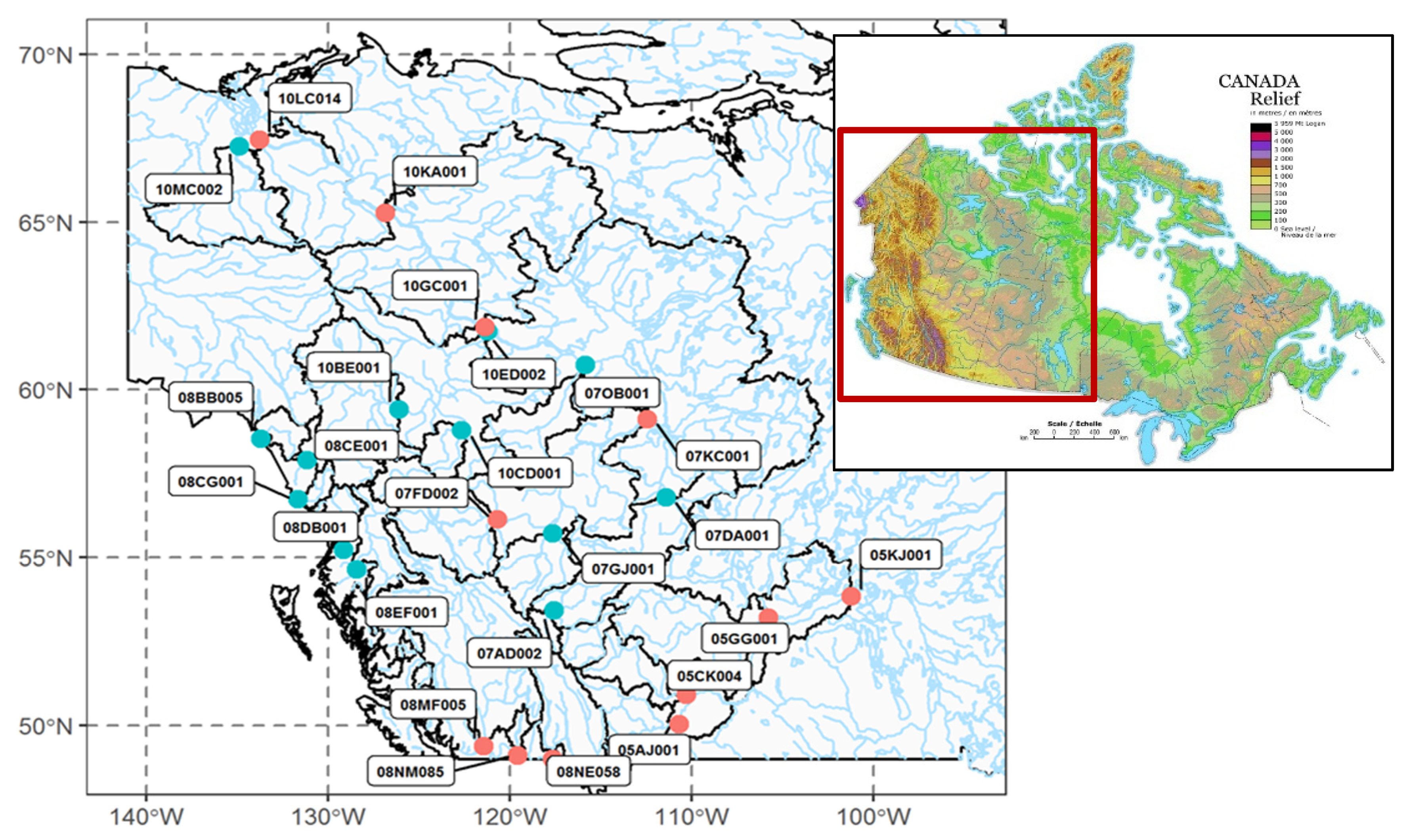
2. Study Area and Data Sets

This study assesses all major river basins across western Canada with a total area of around 2.5 million square kilometers (Figure 1). The region’s physiography is dominated by the Western Cordillera mountains, which are the hydrologic apex of major western North American rivers that drain to the Pacific and Arctic oceans [17]. The major watersheds in the region include the Mackenzie, Yukon, Fraser, Colombia and Saskatchewan, and the flow in each of these river systems is heavily dependent on from mountain snowpack and glaciers [7]. Twenty-five Water Survey of Canada (WSC) hydrometric stations each with drainage areas of more than 7500 square kilometers are utilized. The threshold for the drainage area was chosen to ensure an ample number of grids for the predictor variables described below. Most of the selected stations are located in British Columbia (10), Alberta (6) and the Northwest Territories (7), with the remaining two in Manitoba (1) and Saskatchewan (1). Daily streamflow data from the Water Survey of Canada (WSC) HYDAT database over the 1980–2012 historical period were used to extract AMF and MAMJflow at each of the 25 stations. Basin boundary delineation for each station was obtained from the National Hydrometric Network basin polygons online database [25] and verified with in-house delineations generated by the GRASS GIS tools [26].

Some of the rivers in the study region, such as the Peace River in the Mackenzie basin, tributaries of the Fraser basin and a large part of the Colombia River, are regulated for hydropower production. Similarly, most parts of the Saskatchewan and Okanagan rivers have a system of reservoirs and diversions for irrigation and hydroelectricity [7]. Therefore, while data from 13 of the selected stations represent unregulated natural flows, the 12 remaining stations are designated as regulated with major upstream structure(s) altering the natural flow regime. The level of flow alterations in the regulated stations varies, with the Fraser River at Hope having minor flow alteration, while stations in the Peace and Columbia basins are affected by major flow alterations from upstream dams [27]. Flows in the Saskatchewan and Okanagan basins are also affected by water withdrawal. Nonetheless, the effect of upstream regulation on hydrologic regime usually diminishes with distance downstream of the regulation location. Therefore, regulated stations were included in the study to explore whether the annual peak flows in these locations are influenced by antecedent climatic conditions and if the MLR can still capture the prevailing relationship between the climatic drivers and mean spring and annual peak flows in such basins. Since major regulations in each of those 12 basins started before 1980, the study employed the 1980–2012 historical streamflow data for better consistency. The 25 stations and their drainage areas and geographic coordinates are provided in

Table 1. Hydrometric stations across western Canada used for annual maximum and mean spring flow analysis and MLR modelling.

Number	Station Name	Area (km2)	Lat	Lon	Regulation
10LC014	Mackenzie River at Arctic Red River	1,680,000	67.4560	−133.7533	Yes
10KA001	Mackenzie River at Norman Wells	1,590,000	65.2720	−126.8500	Yes
10GC001	Mackenzie River at Fort Simpson	1,300,000	61.8684	−121.3589	Yes
05KJ001	Saskatchewan River at the Pas	389,000	53.8381	−101.2087	Yes
07KC001	Peace River at Peace Point	293,000	59.1181	−112.4369	Yes
10ED002	Liard River near the Mouth	275,000	61.7427	−121.2280	No
08MF005	Fraser River at Hope	217,000	49.3860	−121.4542	Yes
08NE058	Columbia River at International Boundary	156,000	49.0008	−117.6283	Yes
07DA001	Athabasca River below Fort McMurray	133,000	56.7804	−111.4022	No
05GG001	North Saskatchewan River at Prince Albert	131,000	53.2034	−105.7721	Yes
10BE001	Liard River at lower Crossing	104,000	59.4125	−126.0972	No
07FD002	Peace River near Taylor	101,000	56.1394	−120.6724	Yes
10MC002	Peel River above Fort McPherson	70,600	67.2589	−134.8888	No
05AJ001	South Saskatchewan River at Medicine Hat	56,368	50.0421	−110.6775	Yes
07OB001	Hay River near Hay River	51,700	60.7430	−115.8596	No
07GJ001	Smoky River at Watino	50,300	55.7146	−117.6231	No
05CK004	Red Deer River near Bindloss	47,849	50.9027	−110.2995	Yes
08EF001	Skeena River at Usk	42,300	54.6319	−128.4306	No
08CE001	Stikine River at Telegraph Creek	29,000	57.9003	−131.1597	No
10CD001	Muskwa River near Fort Nelson	20,300	58.7881	−122.6616	No
08DB001	Nass River above Shumal Creek	18,400	55.2623	−129.0850	No
08BB005	Taku River near Juneau	16,700	58.5386	−133.7000	No
07AD002	Athabasca River at Hinton	9760	53.4243	−117.5694	No
08CG001	Iskut River below Johnson River	9500	56.7344	−131.6690	No
08NM085	Okanagan River near Oliver	7540	49.1146	−119.5667	Yes

.

Daily precipitation and daily maximum and minimum air temperature data were obtained from the Pacific Climate Impacts Consortium’s Pacific North-Western North America meteorological (PNWNAmet) dataset [28]. PNWNAmet is a temporally consistent high-resolution gridded daily meteorological dataset at 1/16° spatial resolution for northwestern North America interpolated from temporally consistent long-term homogenized daily station data covering 1945 through 2012. Additionally, historical gridded SWE data were obtained from the NASA Global Modeling and Assimilation Office’s (GMAO) Modern-Era Retrospective Analysis for Research and Applications, Version 2 (MERRA-2) [29]. MERRA-2 provides atmospheric and surface reanalysis data at 50 km spatial resolution from 1980 to the present. As MERRA-2 uses observation-based precipitation data to drive the land surface water budget, its SWE product has lower bias and correlates better against reference data from the Canadian Meteorological Centre than other reanalysis products [30]. For each of the 25 stations, gridded precipitation, temperature and SWE data were extracted and then averaged over the contributing drainage basins. The 1980–2012 time window for the historical period was chosen based on an overlapping time frame between the MERRA-2 data, which starts in 1980, and the PNWNAmet data, which ends in 2012.

3. Application Methods

3.1. Multiple Linear Regression (MLR)

MLR is an extension of ordinary least square regression that can model the linear relationship between several explanatory (predictor) variables and a response (predictand) variable as shown in Equation (1), where i is the index of each observation, y_i is the response variable, x_i represents the explanatory variables, β₀ is the y-intercept, β_p represents slope coefficients and $\mathsf{ϵ}$ is the residual. MLR provides a computationally easy and simple to interpret method of predicting streamflow. The main assumptions are that there is a linear relationship between the predictor and predictand variables and that the predictors are not too highly correlated with each other.

$$y_i={\beta }_0+{\beta }_1{x}_{i1}+{\beta }_2{x}_{i2}+\dots +{\beta }_p{x}_{ip}+\mathsf{ϵ}$$

(1)

While hydrologic processes have nonlinear characteristics, a number of previous studies have shown that MLR between selected predictors and predictand variables can explain most of the variance in catchment responses [21,22,23,24]. In most of the cases, predictors were selected based on an understanding of the physical processes, relevant literature and initial exploratory data analysis. The MLR is also a relatively simple approach for identifying the relative importance of the different potential predictors and the level of significance in the linear relationship established between the predictor and response variables. In this study, the MLR models relate the AMF or MAMJflow (predictands) at each of the 25 hydrometric stations over western Canada with the corresponding basin average values of selected hydroclimatic drivers (predictors). Seven predictors were selected based on the underlying physical processes, relevant literature and initial exploratory data analysis [8,21,24]. As the SWEmax and April 1st SWE are highly correlated, the MLR uses either the magnitude and timing of SWEmax or April 1st SWE, but not both, to avoid multicollinearity. Average spring temperature and precipitation are calculated over the months from March to June (hence MAMJtemp and MAMJpcp respectively). The monthly rates of change in spring temperature (spring warming rate) and precipitation (the spring rate of increasing/decreasing in precipitation) are also calculated as the slope of each variable between March and June (hence MAMJtemp-slope and MAMJpcp-slope, respectively). The nonparametric Spearman’s rank correlation between each predictor and predictand measures the strength and direction of monotonic association between two variables and is estimated using Equation (2), where Di is the difference in ranks between the ith pair of predictor and predictand and n is the number of data pairs (see

Table 2. Hydroclimatic predictors used in the MLR models to predict AMF and MAMJflow at each of the hydrometric stations.

Predictor Name	Abbreviation	Units	Data Source
Annual maximum snow water equivalent	SWEmax	$\mathrm{mm}$	MERRA-2
Date of annual maximum snow water equivalent	SWEmax-date	Date number	MERRA-2
April 1st snow water equivalent	SWEapril 1st	$\mathrm{mm}$	MERRA-2
Average spring temperature	MAMJtemp	$℃$	PNWNAmet
Rate of change in spring temperature	MAMJtemp-slope	$℃/\mathrm{month}$	PNWNAmet
Total spring precipitation	MAMJpcp	$\mathrm{mm}$	PNWNAmet
Rate of change in spring precipitation	MAMJpcp-slope	$\mathrm{mm}/\mathrm{month}$	PNWNAmet

) [31]. The correlation coefficient, r_s, takes values from +1 to −1, and the strength of the rank correlations was analyzed in terms of statistical significance tests at the 5% significance level.

$$r_s=1-\frac{6{{\displaystyle \sum }}_{i=1}^n{D}_i^2}{n\left(n^2-1\right)}$$

(2)

MLR models are fitted to the predictor/predictand data at each station over the 1980 to 2012 historical period, with MAMJpcp, MAMJpcp-slope, MAMJtemp, MAMJtemp-slope as common predictors and either April 1st SWE or SWEmax and its timing as additional predictors and either AMF or MAMJflow as predictand. First, a best subsets regression approach, as implemented in the R leaps package version 3.0, was employed to fit MLR models to all possible combinations of the predictor variables and each of the two predictands. Then, the best fitting MLR model from the pool of all possible combinations with one to five predictor variables (when using April 1st SWE) or one to six predictor variables (when using SWEmax and its timing) were chosen based on the sum-of-squares of residuals [32]. This approach involved an exhaustive comparison of models from each predictor size group and ended in the selection of models with the lowest Akaike information criterion (AIC) [32].

These five or six models each selected from a predictor size group were then compared in terms of their predictive power by repeated k-fold cross-validation, with k = 5 [33]. The k-fold cross-validation procedure divides the limited dataset into k nonoverlapping folds. Each of the k folds is given an opportunity to be used as a held-back test set, whilst all other folds collectively are used as a training dataset. A total of k models were fit and evaluated on the k hold-out test sets and the mean performance was reported. The model with the lowest root-mean-square error (RMSE) from k-fold cross-validation was selected as the final model if it was statistically significant at a p-value of 0.05. All selected models were also tested for their fulfillment of the regression assumptions by computing their variance inflation factors (VIF) with the intention of removing highly correlated predictors with VIF above the most common acceptable threshold of 5 [33,34].

3.2. Predictors’ Relative Importance

Predictor relative importance refers to the quantification of an individual predictor’s contribution to a multiple regression model. To identify which predictors are the most influential in explaining variation in AMF and MAMJflow, the total explained variance, R², of each selected model for a station was decomposed into the proportion explained by each individual predictor using the Lindemann, Merenda and Gold (LMG) method as implemented in the R package relimpo [35]. In addition to the variance explained by each predictor, the percentage of the total variance (explained by the model, R²) that is contributed by each predictor variable provides a measure of the relative importance of each variable. Analysis of these metrics included the frequency of dominant predictors among all station models, where a dominant predictor is defined as the predictor in a model with the highest relative importance. The spatial distribution of dominant predictors was also mapped as it may be a good indicator of the effect of watershed features on predictor–predictand relationships.

3.3. Future Projection of Annual Peak and Spring Flows

To evaluate the applicability of the selected MLR models for estimating future magnitudes of AMF and MAMJflow, climatic predictors derived from the Canadian Regional Climate Model (CanRCM4; Scinocca et al., 2016) [36] under RCP4.5 and RCP8.5 future scenarios were used. The CanRCM4 output used in this study is from the CORDEX Experiments for North America (NAM-22), which is at 0.22° or approximately 25 km resolution and driven by the CanESM2 GCM [36]. Recognizing that RCM outputs usually have systematic biases [37], this study employed the “delta change method”, to account for the biases in future predictor values. Mean projected changes in each of the predictor variables between the 1976–2005 baseline and the two future periods (2041–2070 and 2071–2100) were computed from the CanRCM4 data and then averaged over the basin area contributing to each of the 25 hydrometric stations. The future predictor values for each hydrometric station were computed by applying the CanRCM4 delta changes on the observed values derived from MERRA-2 and PNWNAmet over the historical period as shown in Equation (3) below:

$$\left\{\begin{array}{c}{\mathsf{\Delta }}_m=CanRCM{4}_{future}-CanRCM{4}_{baseline}\mathrm{or}{\mathsf{\Delta }}_m=CanRCM{4}_{future}/CanRCM{4}_{baseline}\hfill \\ Scenari{o}_{future}=Observe{d}_{historical}+{\mathsf{\Delta }}_m\mathrm{or}Scenari{o}_{future}=Observe{d}_{historical}\ast {\mathsf{\Delta }}_m\hfill \end{array}\right.$$

(3)

Changes between the baseline and future periods were calculated in terms of ratios for SWEmax, SWEapril 1st, MAMJpcp, MAMJpcp-slope and MAMJtemp-slope or differences for MAMJtemp and SWEmax-date and applied to the historical observations to obtain the corresponding future projections (Equation (3)). The MLR model for each station was then forced with the adjusted hydroclimatic predictors to compute AMF and MAMJflow corresponding to the different RCP scenarios and future periods.

4. Results and Discussion

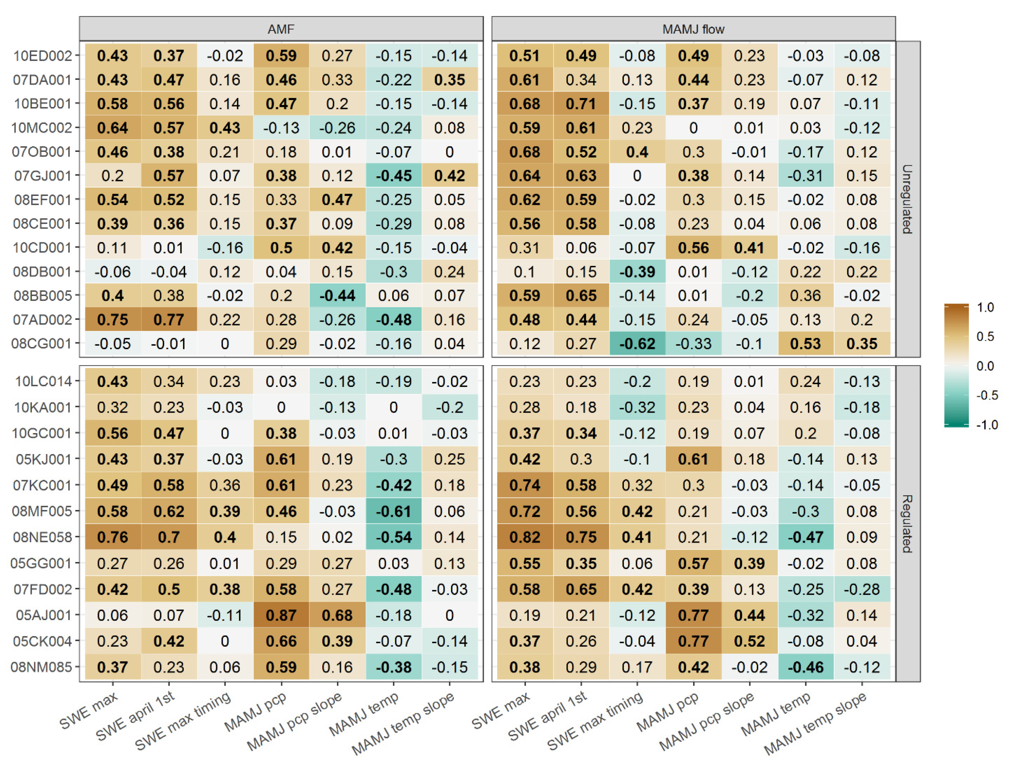
4.1. Spearman’s Rank Correlation

The Spearman correlations between the selected predictors and predictands at each of the 25 hydrometric stations are presented in Figure 2. The correlation coefficients (as expressed by r_s) indicate that both the AMF and MAMJflow at most of the stations are positively correlated with SWEmax, April 1st SWE and spring precipitation (MAMJpcp) and negatively correlated with mean spring temperature (MAMJtemp), though the correlation strength varies. However, there are some smaller watershed stations in the Pacific coastal region (e.g., 08CG001 and 08DB001) and some regulated stations (e.g., 05AJ001) that show weaker correlations with these predictors. This is mainly because peak flows in those coastal watersheds are less controlled by snowmelt and more by rainfall, and in regulated stations, they are affected by regulations. The correlations with SWEmax timing (SWEmax-date) and mean spring precipitation and temperature slopes (MAMJtemp-slope and MAMJpcp-slope, respectively) are generally weaker, although they are significant at some specific stations. While there are some differences in the correlation matrix between regulated and unregulated stations, the results do not indicate one group as being more correlated than the other.

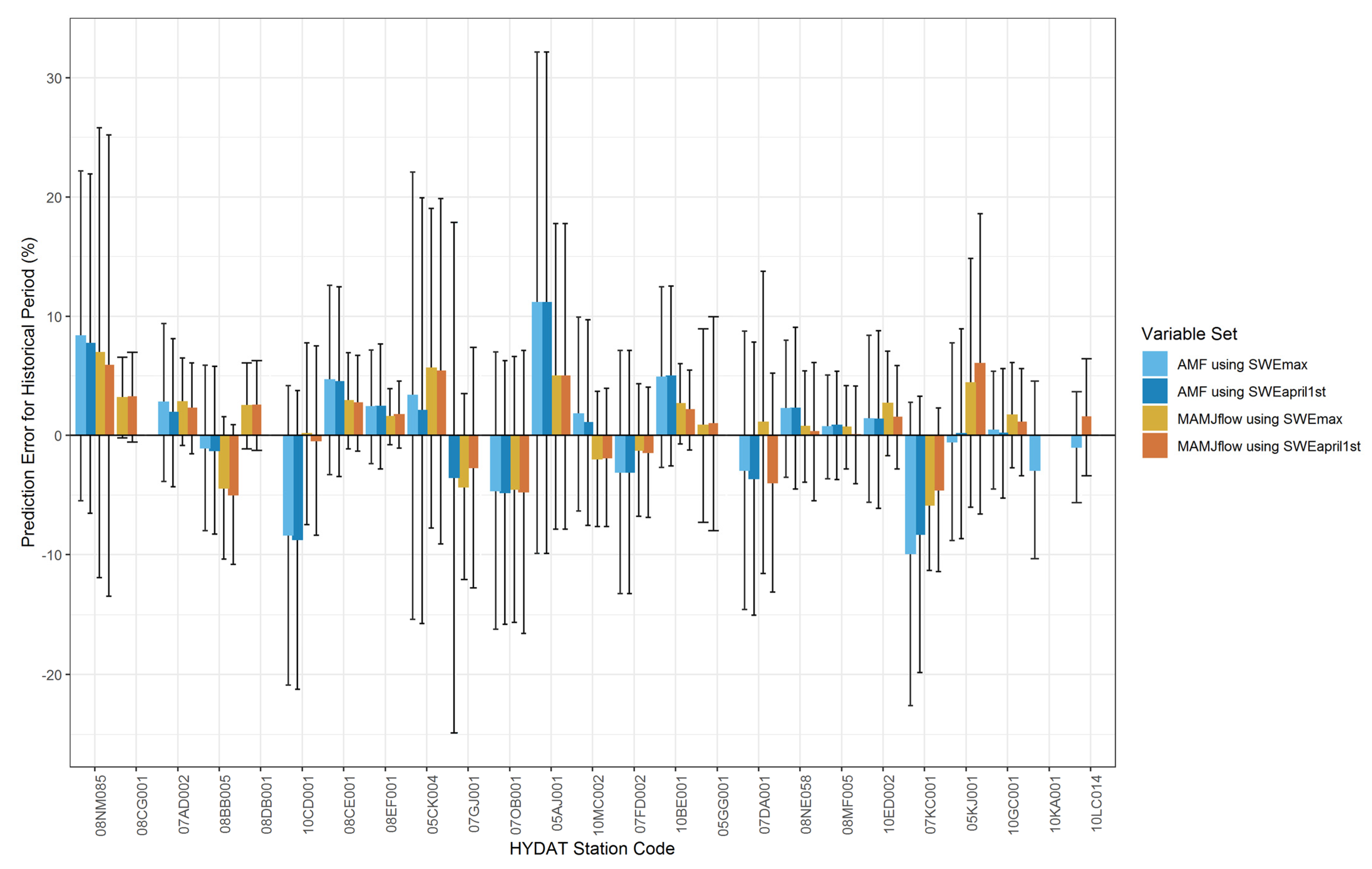
4.2. MLR Model Performances

The MLR models fitted to each of the 25 stations and four combinations (with either AMF or MAMJflow as predictand and either SWEmax and its timing or April 1st SWE as predictors) over the 1980 to 2012 period resulted in a total of 100 optimized models. None of the selected models were found to have problematic multicollinearity, with VIF less than 5 indicating no significant correlation between predictor variables [31]. This may be explained in part by the careful initial variable selection which included the decision to build models with either SWEmax or April 1st SWE but not both variables. However, 12 models (9 for AMF and 3 for MAMJflow, out of the 100) that are not statistically significant (p-value > 0.05) were removed, resulting in the final selection of 88 MLR models. Some of the stations where the MLR models are not statistically significant are located in the Pacific coastal region (e.g., 08CG001, 08DB001), while others are in the interior of the Mackenzie basin with relatively large drainage areas that are affected by the Peace River regulations (e.g., 10KA001, 10LC014). Nonetheless, MLR models also show good performances in most other regulated basins comparable to those of the nonregulated ones. The list of all selected models corresponding to each hydrometric station along with models’ R² and p-values is provided in Supplementary Materials.

The MLR performances are presented in Figure 3, which summarizes the mean percentage differences between model-predicted and observed AMF and MAMJflow over the 1980–2012 historical period for those models with p-value < 0.05 along with error bars indicating the 95% confidence interval. The results generally indicate a good model performance with the historical period mean prediction error at most stations being within ±10% of the observed values. However, few stations have prediction errors in some years in the order of ±20%. It is also not surprising that most of the stations with relatively higher prediction error are located in highly regulated watersheds (e.g., 08NM085 and 05AJ001 have water withdrawals, and 07KC001 is affected by reservoir regulation). Other factors including the size and hypsometry of the contributing watershed may also affect the performance of the MLR models. However, since the effects of the different factors are overlapping, it is hard to clearly identify the specific reason for some of the unsatisfactory performances. The error in predicting AMF is relatively larger than that in predicting MAMJflow. This is also expected because MAMJflow is averaged flow over four months where the daily variations are smoothened out while AMF is a peak of daily flows occurring at any time during the spring or summer high flow seasons. For the majority of the stations, the MLR models with either SWEmax or April 1st SWE as predictor show similar performances, except in a few stations where using April 1st SWE resulted in a relatively smaller prediction error.

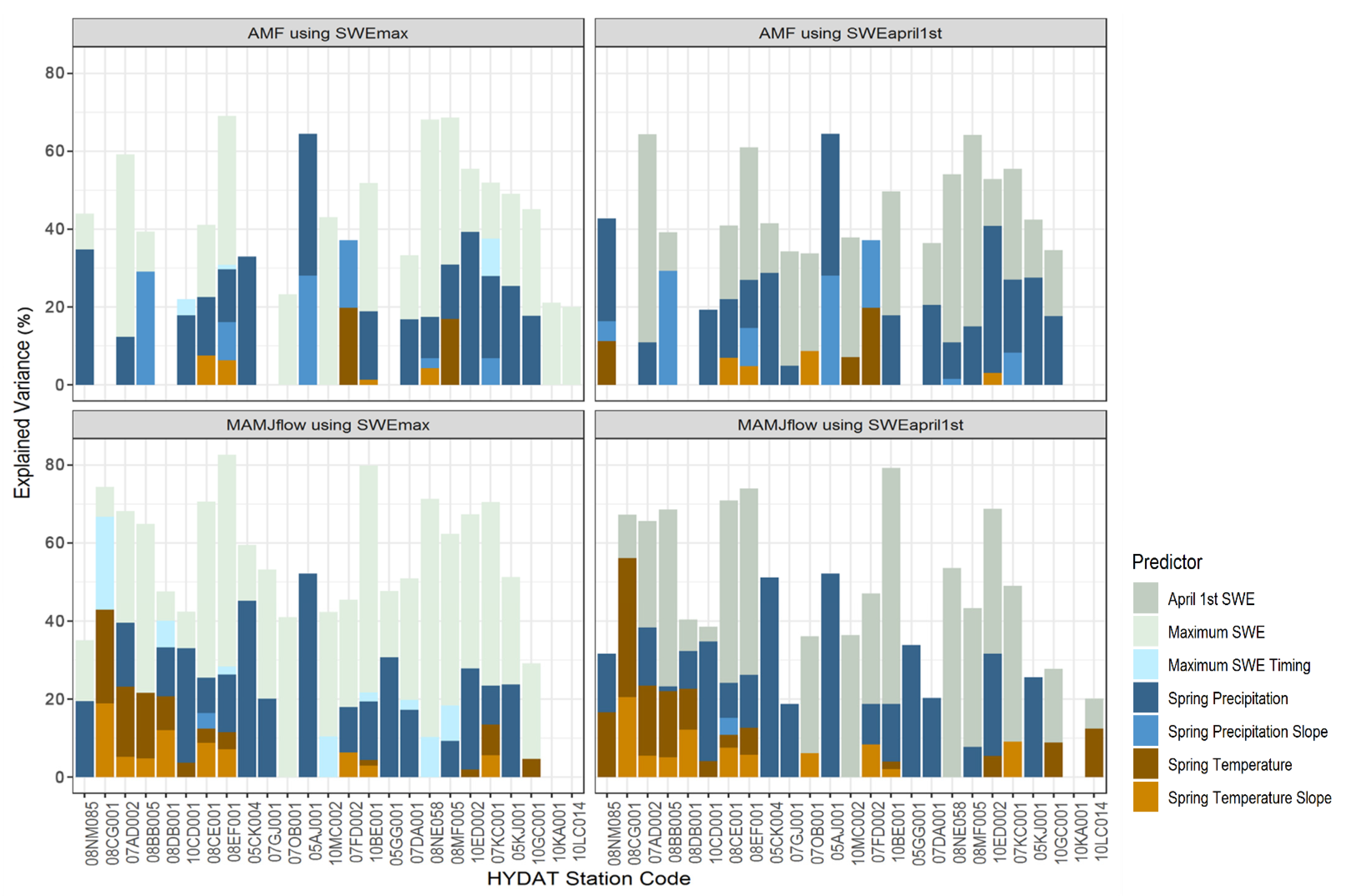
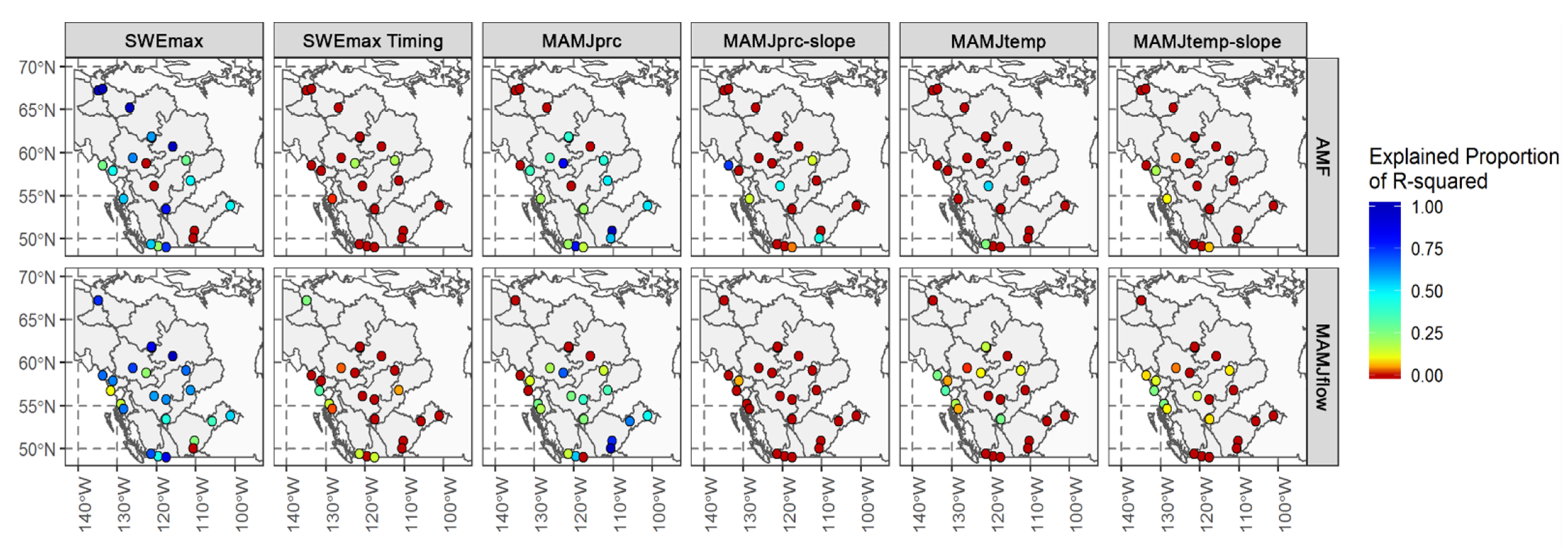
4.3. Predictors’ Relative Importance

Figure 4 shows the relative importance of each climatic predictor in the MLR models in explaining the variances of the predictands at each hydrometric station. Top and bottom panels correspond to AMF and MAMJflow while left and right sides display SWEmax and April 1st SWE, respectively. For the majority of stations, April 1st SWE or SWEmax contributed the highest proportion of explained variance, indicating the relatively higher importance of snow accumulation in predicting AMF and MAMJflow. For most stations, MAMJPrc has the second-highest predictor importance. The proportion of explained variance in predicting both AMF and MAMJflow averaged across all stations is in the order of 44% for April 1st SWE and 51.7% for SWEmax. This is followed by MAMJprc with the proportion of explained variance ranging between 29.4% and 37.6% under the different categories. However, for some regulated stations (e.g., 08NM085, 05CK004, 05AJ001, 05KJ001), the predictor importance of MAMJprc is higher than that of SWE. MAMJprc-slope contributed more to the explained variance of AMF while MAMJtemp and MAMJtemp-slope contributed more to the explained variance of MAMJflow at about half of the stations. While MAMJprc-slope contributes to around 10% of the explained variance in predicting AMF, its contribution to predicting MAMJflow is almost nonexistent (<0.3%). The results also show that the contribution of MAMJtemp and MAMJtemp-slope to the explained variance is relatively small and with higher contribution to predicting MAMJflow (5–13%) than to AMF (2–5%).

Similarly, Figure 5 presents the spatial distribution of predictors’ relative importance for the AMF and MAMJflows at each of the 25 stations over western Canada. Once again the figure shows SWEmax as the most important predictor at most stations (21/25 for AMF and 24/25 for MAMJflow), followed by MAMJprc, which is also an important predictor (20/25 for AMF and 19/25 for MAMJflow). MAMJtemp and MAMJtemp-slope are important predictors of MAMJflow for about one-third of the stations, mostly located in the middle part of the study region, while their contribution to predicting AMF is limited to a couple of stations. MAMJprc-slope is important in predicting AMF in the southern and Pacific coast regions but not that important in predicting MAMJflow in most parts of the study region. The contribution of SWEmax timing in predicting both AMF and MAMJflows is limited only to a few stations. The generally smaller importance of spring temperature and its rate of increase in predicting AMF is an indication that spring peak flows in most basins are affected more by accumulated snow and spring precipitation than temperature. The predictability of MAMJflow is also mostly dependent on more variables than that of AMF, a possible reason for the MAMJflow models being more robust with relatively smaller prediction errors. While the importance of SWEmax in predicting flow is higher towards the northern part of the study region, the importance of MAMJprc is higher towards the south, possibly resulting from the effect of temperature on partitioning precipitation into rain and snow. In general, the results presented in Figure 5 show that predictors’ relative importance is spatially variable and cannot be generalized for the whole region.

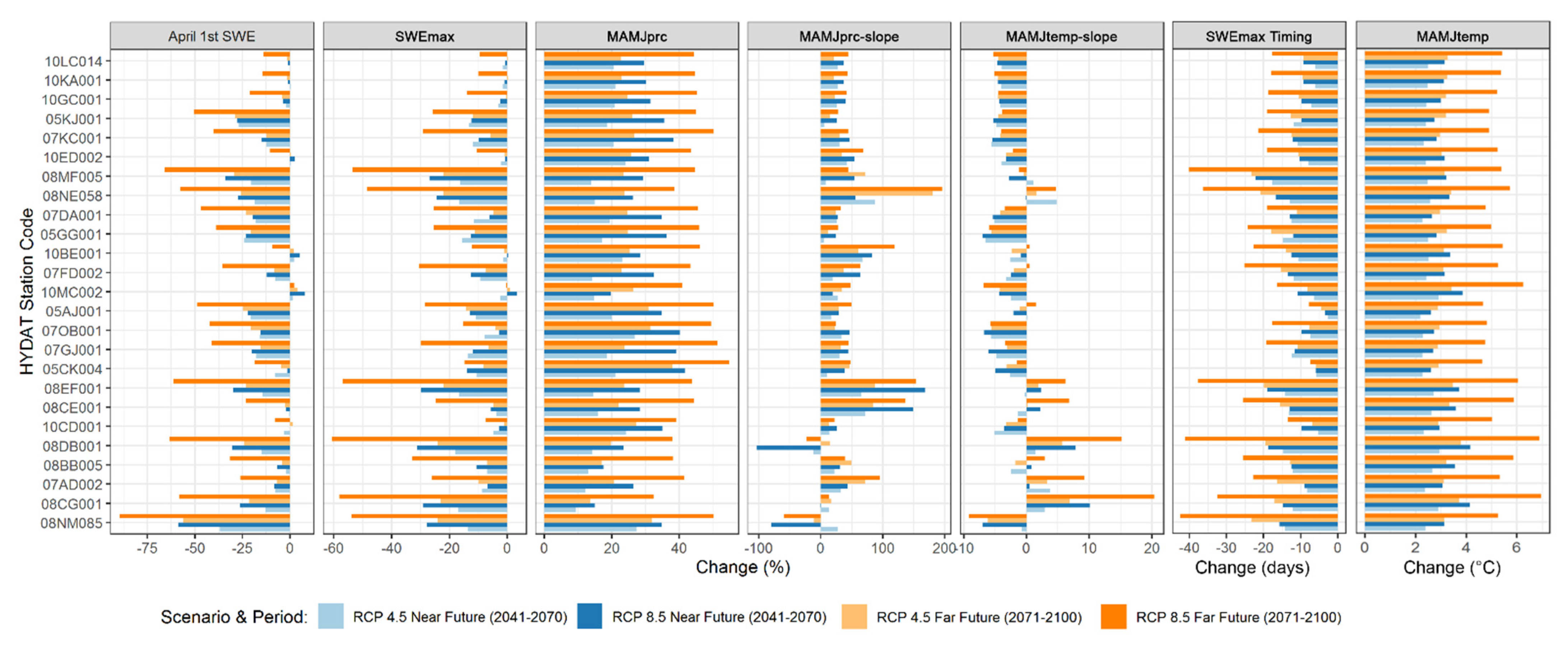
4.4. Projected Changes in Hydroclimatic Variables

Figure 6 shows mean CanRCM4 projected changes in each of the predictor variables between the 1976–2005 baseline and the two future periods (2041–2070 and 2071–2100) for the two scenarios (RCP4.5 and RCP8.5). The results indicate that both MAMJpcp and MAMJtemp are projected to increase from 10% to 50% for the former and from 2 to 7 °C for the latter depending on the RCP scenarios and the future time windows considered. As expected, the biggest increases for both precipitation and temperature occur under RCP8.5 and far future (2071–2100) period while the smaller increases correspond to RCP4.5 and the near future (2041–2070) period. While there are some regional variations in the projected changes in spring precipitation and temperature with slightly higher increases in the northern than the southern basins, the differences are relatively small.

SWEmax and April 1st SWE are both projected to decrease in the majority of the basins under both scenarios and time periods with values ranging from −80% to +5%. The greatest decreases are mostly in the Fraser, Colombia, and Pacific coast basins, while the smallest decreases or even slight increases correspond to the most northern basins, as was also found in previous studies [15,38]. At the same time, SWEmax timing is projected to advance by about 5 to 25 days in all river basins. MAMJpcp-slope increases in almost all basins (except two), indicating more increase in precipitation in the later part rather than the earlier part of spring. In contrast, MAMJtemp-slope show decreases for most basins, indicating higher increases in early spring than late spring, except for a few southern stations where the reverse is true. In general, while the overall direction of projected changes in the predictor variables over most parts of the study region is similar, there are some north-to-south variations in the magnitude of those changes.

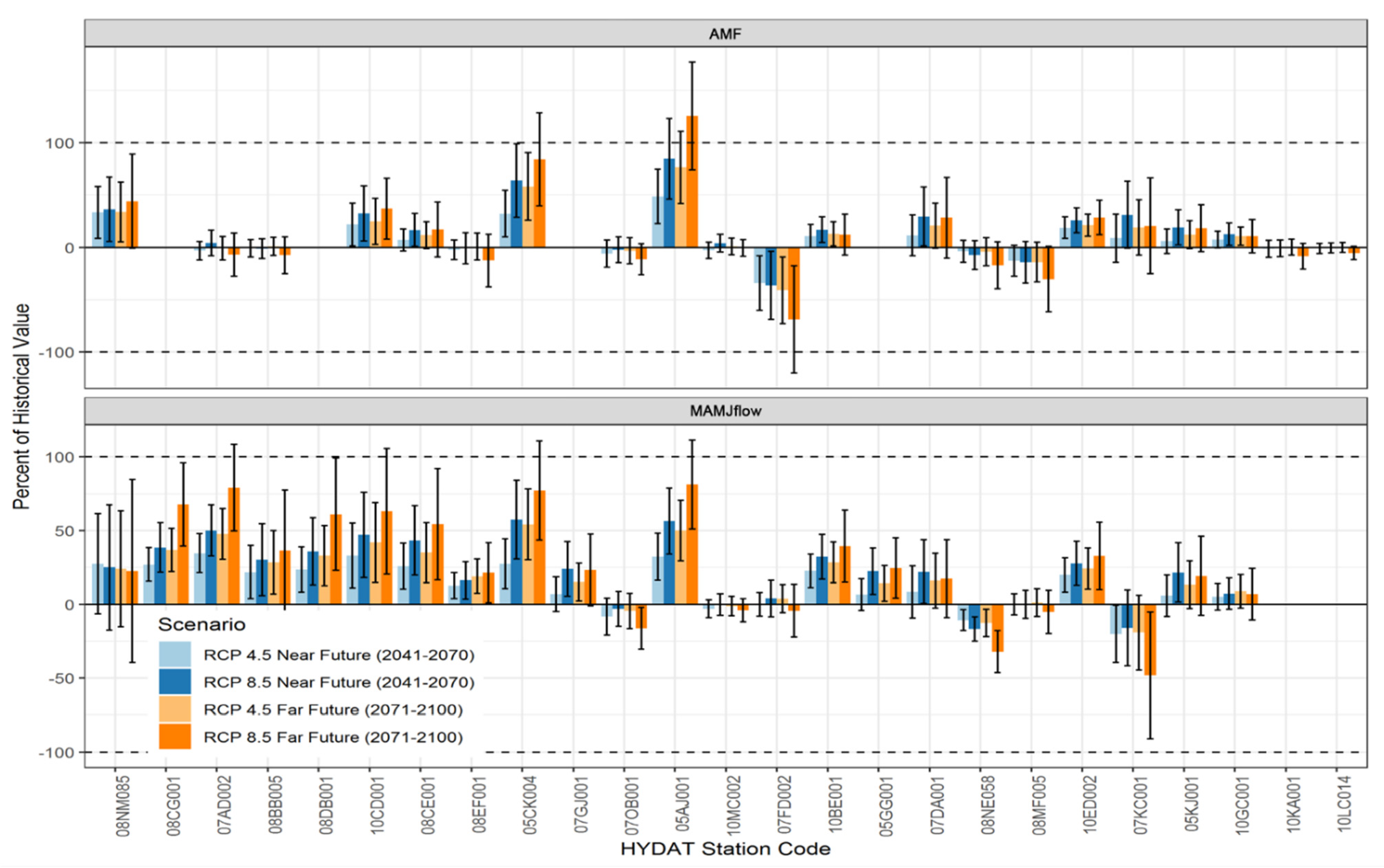
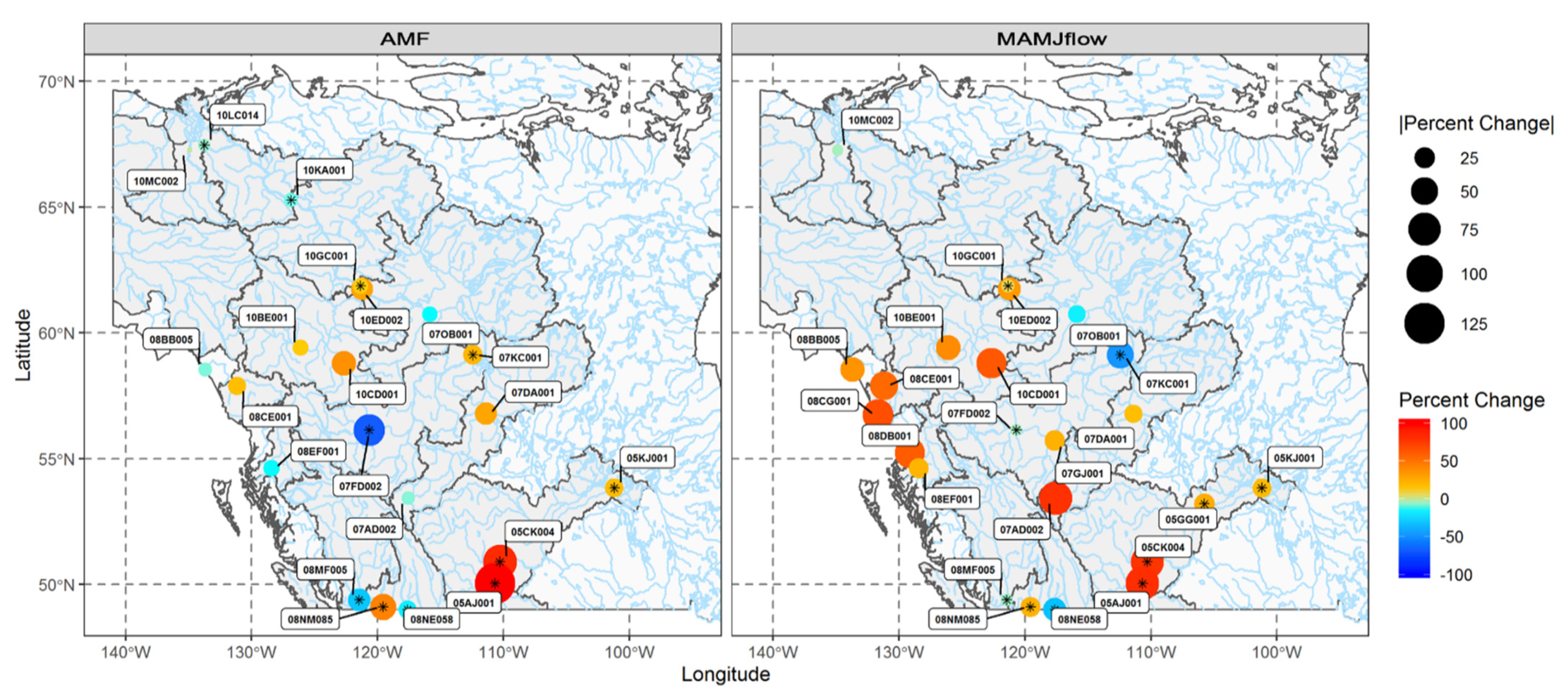
4.5. Projected Changes in AMF and MAMJflow

Future projections of AMF and MAMJflow were computed using the MLR models developed for the historical period, with delta changes from the CanRCM4 projections under the two RCP scenarios applied on the observed predictor values (Equation (3)). The results indicate overall projected increases in both the AMF and MAMJflow for most of the stations, with a few stations showing no change or some decreases (Figure 7). For RCP8.5 and the far future period, the average increase in AMF (12%, ranging from −69% to +126%) has more spatial variability than that of MAMJflow (28%, ranging from −48% to +81%) (Figure 8). The largest percent increases in both are located in Saskatchewan (05AJ001, 05CK004), although large increases in MAMJflow are also projected in the Athabasca (07AD002) and other northwestern rivers. The largest decreases in both AMF and MAMJflow are located at the Peace River at Taylor (07FD002) and Peace Point (07KC001), respectively. Most northern stations are projected to have relatively smaller percentage changes in AMF compared to the south, although the absolute magnitude of these changes can be larger for those with relatively larger flow magnitudes, such as in the Mackenzie River mainstem stations.

Projected increases in AMF are mostly located in the interior of western Canada, while increases in MAMJflow are found throughout the region. However, the projected AMF in the coastal basins could be subject to large uncertainties since peak flow events in the region are sometimes influenced by atmospheric rivers, which is not taken into account in the MLR model [39]. No clear pattern was found differentiating the results from regulated and unregulated stations since some regulated stations (e.g., in Peace, Fraser and Colombia rivers) show projected decreases in AMF and MAMJflow while other regulated stations (e.g., South Saskatchewan and Liard rivers) show increases. The wide variation in the direction and magnitude of projected changes in AMF among the river basins could partly be due to changes in the synchrony of mainstem and tributary streamflow during high-flow periods at the mainstem–tributary confluence [40]. Decreasing synchrony may dampen the forced increases in AMFs along mainstem stations, but its relative effects may vary in space and time, as well as in future climate scenarios.

A comparison of the projected changes in flows using the MLR models and future climate projections (applying delta change method) with those of other previous studies using process-based hydrological models driven by statistically downscaled GCMs shows both agreement and disagreement depending on basin characteristics. For example, the directions of MLR-projected changes, such as increases in AMF and MAMJflow for the unregulated Liard (10BE001, 10ED001) and Athabasca (07DA001) basins, are consistent with previous studies in the two basins using process-based hydrologic models [15,41]. Similarly, for the mildly regulated station in the Fraser basin (08MF005), the MLR model projections of decreases in AMF and no change in MAMJflow are comparable with the projections of decreases in AMF and some increases in MAMJflow of Shrestha et al. [27]. However, the MLR model projections for the Peace basin (07KC001, 07FD002) are not consistent with the results of Schnorbus et al. [42], which showed projected increases in both AMF and MAMJflow. Likewise, the MLR projected decreases in AMF and MAMJflow at another regulated station in the Columbia River (08NE058), in contrast to the projected increases for the same basin reported by Werner et al. [43]. The discrepancies could be partly explained by the fact that both the Peace and Columbia rivers are highly regulated by large hydroelectric dams/reservoirs. Schnorbus et al. [42] and Werner et al. [43] also used naturalized flows, while the MLR models are based on the regulated flows. Besides, the lack of representation of physical processes in the MLR model is one of its limitations in extrapolating beyond the range of historical observation affecting flow projections for some basins. Therefore, the overall ability of the MLR model to project AMF and MAMJflow may be limited, especially when applied to regulated basins.

5. Summary and Conclusions

Flows originating from cold and mountainous watersheds are highly dependent on their snow regimes that are determined by temperature and precipitation patterns over the region. Climatic variations generally affect the mean seasonal flows and the magnitude and timing of peak streamflow events with implications on infrastructures and ecosystem services. This study applied the MLR approach for assessing the climatic controls of AMF and MAMJflow in 25 western Canadian river basins using multiple station-specific hydroclimatic predictors. The analysis indicated that the basin-integrated SWEmax or April 1st SWE and mean spring precipitation (MAMJPr) are the most prominent predictors of AMF and MAMJflow throughout the region, together explaining over 80% of the predictand’s variance. The proportion of explained variance is in the order of 44% for April 1st SWE and 51.7% for SWEmax, followed by MAMJprc explaining between 29.4% and 37.6% of the predictand’s variance. However, predictors’ relative importance was spatially variable and could not be generalized for the whole region. While the relative importance of SWEmax in predicting flow is higher towards the north and that of MAMJprc is higher towards the south, the relative importance of MAMJtemp is mostly higher in the middle part of the study region. The best-fitting MLR models were statistically significant at a p-value of 0.05 at the majority (88%) of the stations, and mean prediction errors over the historical period were below ±10% at most stations (although a few stations had prediction errors ranging in the order of ±20%).

The results of this study are highly relevant to other regions of the world where runoff processes are dominated by mountain snowpack. The main lesson is that while winter snow accumulation and spring precipitation are the major drivers of mean spring and annual peak flows in cold mountainous watersheds, their relative contribution to predictability largely depends on the location and other physiographic characteristics of the watersheds. Other studies have also shown that the transformation from snow accumulation to runoff generation in cold regions is dominated by snowmelt and infiltration processes that are highly heterogeneous [44]. In particular, direct human impacts, such as regulation and diversion in the basin, can alter its flow regime and affect the dependency between those predictor and response variables. Therefore, there is a need to carefully consider physiographic characteristics as well as human impacts in using regression models for streamflow simulation.

A warming climate will bring a shift in precipitation from snow towards rain, affecting the snowpack volume and snowmelt timing. Therefore, by adjusting the snowpack together with precipitation and temperature based on CanRCM4 projections, the MLR models were tested to see if they can be applied to predict future changes in AMF and MAMJflow. CanRCM4 outputs show a general increase in mean spring temperature (2 to 7 °C) and precipitation (10% to 55%) and an overall decrease in SWEmax and April 1st SWE for all but two river basins (+5% to −95%) by the end of this century. Application of the MLR models with adjusted hydroclimatic predictors revealed considerable spatial variations, with the projected increase in spring precipitation mostly compensating the opposite effect of increasing spring temperature and decrease in SWE and resulting in AMF changes ranging from −69% to +126% and MAMJflow changes ranging from −48% to +81%. Projected changes are mostly higher for the RCP8.5 and end-of-century scenarios. Projected changes in MAMJflow across the region are more consistent than those of AMF. Other things being equal, change in phase of precipitation from snow towards rain (because of increasing temperature) usually decreases the mean streamflow [1]. However, the current study indicated that the projected increase in precipitation can sometimes compensate for the effect of the decreasing fraction of snowfall and may result in an increase in spring flow.

Comparisons of the MLR model projections with some previous studies using process-based hydrological models driven by statistically downscaled GCMs show good agreement in the direction of change for most of the unregulated rivers, while there are substantial disagreements for the regulated river basins. This is in part due to the lack of physical representation in these models, as well as limitations in extrapolating future flow magnitudes beyond the range of historical observation. Therefore, there is a need to exercise caution in the use of such statistical models for projecting future changes, especially in regulated basins. More research is needed to better understand the extent of the limitation and ways of incorporating relevant information in the modelling process to reduce those limitations. Future research may also look at possible improvements by applying nonlinear methods such as artificial neural networks (ANNs) and other machine learning techniques.

References

1. Berghuijs, W.R.; Woods, R.A.; Hrachowitz, M. A precipitation shift from snow towards rain leads to a decrease in streamflow. Nat. Clim. Chang. 2014, 4, 583–586. [Google Scholar] [CrossRef] [Green Version]
2. Burn, D.H. Climatic influences on streamflow timing in the headwaters of the Mackenzie River Basin. J. Hydrol. 2008, 352, 225–238. [Google Scholar] [CrossRef]
3. Dudley, R.W.; Hodgkins, G.A.; McHale, M.R.; Kolian, M.J.; Renard, B. Trends in snowmelt-related streamflow timing in the conterminous United States. J. Hydrol. 2017, 547, 208–221. [Google Scholar] [CrossRef] [Green Version]
4. Sandink, D. Urban flooding and ground-related homes in Canada: An overview. J. Flood Risk Manag. 2016, 9, 208–223. [Google Scholar] [CrossRef]
5. Dibike, Y.; Prowse, T.; Bonsal, B.; O’Neil, H. Implications of future climate on water availability in the western Canadian river basins. Int. J. Climatol. 2017, 37, 3247–3263. [Google Scholar] [CrossRef]
6. Bawden, A.J.; Burn, D.H.; Prowse, T.D. Recent changes in patterns of western Canadian river flow and association with climatic drivers. Hydrol. Res. 2015, 46, 551–565. [Google Scholar] [CrossRef]
7. Bonsal, B.; Shrestha, R.R.; Dibike, Y.; Peters, D.L.; Spence, C.; Mudryk, L.; Yang, D. Western Canadian Freshwater Availability: Current and Future Vulnerabilities. Environ. Rev. 2020, 28, 528–545. [Google Scholar] [CrossRef]
8. Kang, D.H.; Gao, H.; Shi, X.; ul Islam, S.; Déry, S.J. Impacts of a rapidly declining mountain snowpack on streamflow timing in Canada’s Fraser River basin. Sci. Rep. 2016, 6, 1–8. [Google Scholar] [CrossRef] [PubMed] [Green Version]
9. Barnett, T.P.; Adam, J.C.; Lettenmaier, D.P. Potential impacts of a warming climate on water availability in snow-dominated regions. Nature 2005, 438, 303–309. [Google Scholar] [CrossRef]
10. Buttle, J.M.; Allen, D.M.; Caissie, D.; Davison, B.; Hayashi, M.; Peters, D.L.; Pomeroy, J.W.; Simonovic, S.; St-Hilaire, A.; Whitfield, P.H. Flood processes in Canada: Regional and special aspects. Can. Water Resour. J. 2016, 41, 7–30. [Google Scholar] [CrossRef]
11. Erler, A.R.; Peltier, W.R. Projected changes in precipitation extremes for western Canada based on high-resolution regional climate simulations. J. Clim. 2016, 29, 8841–8863. [Google Scholar] [CrossRef]
12. Shrestha, R.R.; Cannon, A.J.; Schnorbus, M.A.; Alford, H. Climatic controls on future hydrologic changes in a subarctic river basin in Canada. J. Hydrometeorol. 2019, 20, 1757–1778. [Google Scholar] [CrossRef]
13. Najafi, M.R.; Zwiers, F.; Gillett, N. Attribution of the Observed Spring Snowpack Decline in British Columbia to Anthropogenic Climate Change. J. Clim. 2017, 30, 4113–4130. [Google Scholar] [CrossRef]
14. Dibike, Y.; Eum, H.I.; Prowse, T. Modelling the Athabasca watershed snow response to a changing climate. J. Hydrol. Reg. Stud. 2018, 15, 134–148. [Google Scholar] [CrossRef]
15. Shrestha, R.R.; Bonsal, B.R.; Bonnyman, J.M.; Cannon, A.J.; Najafi, M.R. Heterogeneous snowpack response and snow drought occurrence across river basins of northwestern North America under 1.0 °C to 4.0 °C global warming. Clim. Chang. 2021, 164, 1–21. [Google Scholar] [CrossRef]
16. Stewart, I.T. Changes in snowpack and snowmelt runoff for key mountain regions. Hydrol. Process. 2009, 23, 78–94. [Google Scholar] [CrossRef]
17. Rood, S.B.; Pan, J.; Gill, K.M.; Franks, C.G.; Samuelson, G.M.; Shepherd, A. Declining summer flows of Rocky Mountain rivers: Changing seasonal hydrology and probable impacts on floodplain forests. J. Hydrol. 2008, 349, 397–410. [Google Scholar] [CrossRef]
18. Milner, A.M.; Khamis, K.; Battin, T.J.; Brittain, J.E.; Barrand, N.E.; Füreder, L.; Cauvy-Fraunié, S.; Gíslason, G.M.; Jacobsen, D.; Hannah, D.M.; et al. Glacier shrinkage driving global changes in downstream systems. Proc. Natl. Acad. Sci. USA 2017, 114, 9770–9778. [Google Scholar] [CrossRef] [PubMed] [Green Version]
19. Cunderlik, J.M.; Ouarda, T.B. Trends in the timing and magnitude of floods in Canada. J. Hydrol. 2009, 375, 471–480. [Google Scholar] [CrossRef]
20. Dibike, Y.; Eum, H.I.; Coulibaly, P.; Hartmann, J. Projected Changes in the Frequency of Peak Flows along the Athabasca River: Sensitivity of Results to Statistical Methods of Analysis. Climate 2019, 7, 88. [Google Scholar] [CrossRef] [Green Version]
21. Curry, C.L.; Zwiers, F.W. Examining controls on peak annual streamflow and floods in the Fraser River Basin of British Columbia. Hydrol. Earth Syst. Sci. 2018, 22, 2285–2309. [Google Scholar] [CrossRef] [Green Version]
22. Tsakiri, K.; Marsellos, A.; Kapetanakis, S. Artificial neural network and multiple linear regression for flood prediction in Mohawk River, New York. Water 2018, 10, 1158. [Google Scholar] [CrossRef] [Green Version]
23. Moradi, A.M.; Dariane, A.B.; Yang, G.; Block, P. Long-range reservoir inflow forecasts using large-scale climate predictors. Int. J. Climatol. 2020, 40, 5429–5450. [Google Scholar] [CrossRef]
24. Shrestha, R.R.; Pesklevits, J.; Yang, D.; Peters, D.L.; Dibike, Y.B. Climatic Controls on Mean and Extreme Streamflow Changes Across the Permafrost Region of Canada. Water 2021, 13, 626. [Google Scholar] [CrossRef]
25. Environment and Climate Change Canada. National Hydrometric Network Basin Polygons. Available online: https://open.canada.ca/data/en/dataset/0c121878-ac23-46f5-95df-eb9960753375 (accessed on 15 May 2019).
26. Neteler, M.; Bowman, M.H.; Landa, M.; Metz, M. GRASS GIS: A multi-purpose open source GIS. Environ. Model Softw. 2012, 31, 124–130. [Google Scholar] [CrossRef] [Green Version]
27. Shrestha, R.R.; Schnorbus, M.A.; Werner, A.T.; Berland, A.J. Modelling spatial and temporal variability of hydrologic impacts of climate change in the Fraser River basin, British Columbia, Canada. Hydrol. Process. 2012, 26, 1840–1860. [Google Scholar] [CrossRef]
28. Werner, A.T.; Schnorbus, M.A.; Shrestha, R.R.; Cannon, A.J.; Zwiers, F.W.; Dayon, G.; Anslow, F. A long-term, temporally consistent, gridded daily meteorological dataset for northwestern North America. Sci. Data 2019, 6, 1–16. [Google Scholar] [CrossRef] [Green Version]
29. Gelaro, R.; McCarty, W.; Suárez, M.J.; Todling, R.; Molod, A.; Takacs, L.; Randles, C.A.; Darmenov, A.; Bosilovich, M.G.; Reichle, R.; et al. The modern-era retrospective analysis for research and applications, version 2 (MERRA-2). J. Clim. 2017, 30, 5419–5454. [Google Scholar] [CrossRef]
30. Reichle, R.H.; Draper, C.S.; Liu, Q.; Girotto, M.; Mahanama, S.P.; Koster, R.D.; De Lannoy, G.J. Assessment of MERRA-2 land surface hydrology estimates. J. Clim. 2017, 30, 2937–2960. [Google Scholar] [CrossRef] [Green Version]
31. Gaál, L.; Szolgay, J.; Kohnová, S.; Hlavčová, K.; Parajka, J.; Viglione, A.; Merz, R.; Blöschl, G. Dependence between flood peaks and volumes: A case study on climate and hydrological controls. Hydrol. Sci. J. 2015, 60, 968–984. [Google Scholar] [CrossRef] [Green Version]
32. Hastie, T.; Tibshirani, R.; Friedman, J. The Elements of Statistical Learning: Data Mining, Inference, and Prediction, 2nd ed.; Springer Science & Business Media: Berlin, Germany, 2009; pp. 57–58. [Google Scholar]
33. Laio, F.; Di Baldassarre, G.; Montanari, A. Model selection techniques for the frequency analysis of hydrological extremes. Water Resour. Res. 2009, 45, W07416. [Google Scholar] [CrossRef]
34. James, G.; Witten, D.; Hastie, T.; Tibshirani, R. An Introduction to Statistical Learning with Applications in R; Springer: New York, NY, USA, 2013; pp. 59–126. [Google Scholar]
35. Schoups, G.; Van de Giesen, N.C.; Savenije, H.H.G. Model complexity control for hydrologic prediction. Water Resour. Res. 2008, 44, W00B03. [Google Scholar] [CrossRef] [Green Version]
36. Grömping, U. Relative importance for linear regression in R: The package relaimpo. J. Stat. Softw. 2006, 17, 1–27. [Google Scholar] [CrossRef] [Green Version]
37. Scinocca, J.F.; Kharin, V.V.; Jiao, Y.; Qian, M.W.; Lazare, M.; Solheim, L.; Flato, G.M.; Biner, S.; Desgagne, M.; Dugas, B. Coordinated global and regional climate modeling. J. Clim. 2016, 29, 17–35. [Google Scholar] [CrossRef]
38. Shrestha, R.R.; Schnorbus, M.A.; Werner, A.T.; Zwiers, F.W. Evaluating hydroclimatic change signals from statistically and dynamically downscaled GCMs and hydrologic models. J. Hydrometeorol. 2014, 15, 844–860. [Google Scholar] [CrossRef]
39. Sharma, A.R.; Déry, S.J. Linking atmospheric rivers to annual and extreme river runoff in British Columbia and southeastern Alaska. J. Hydrometeorol. 2020, 21, 2457–2472. [Google Scholar] [CrossRef]
40. Rupp, D.E.; Chegwidden, O.S.; Nijssen, B.; Clark, M.P. Changing river network synchrony modulates projected increases in high flows. Water Resour. Res. 2021. [Google Scholar] [CrossRef]
41. Eum, H.I.; Dibike, Y.; Prowse, T. Climate-induced alteration of hydrologic indicators in the Athabasca River Basin, Alberta, Canada. J. Hydrol. 2017, 544, 327–342. [Google Scholar] [CrossRef]
42. Schnorbus, M.; Werner, A.; Bennett, K. Impacts of climate change in three hydrologic regimes in British Columbia, Canada. Hydrol. Process. 2014, 28, 1170–1189. [Google Scholar] [CrossRef]
43. Werner, A.T.; Schnorbus, M.A.; Shrestha, R.R.; Eckstrand, H.D. Spatial and Temporal Change in the Hydro-Climatology of the Canadian Portion of the Columbia River Basin under Multiple Emissions Scenarios. Atmos. Ocean 2013, 51, 357–379. [Google Scholar] [CrossRef]
44. Shook, K.; Pomeroy, J.; van der Kamp, G. The transformation of frequency distributions of winter precipitation to spring streamflow probabilities in cold regions; case studies from the Canadian Prairies. J. Hydrol. 2015, 521, 395–409. [Google Scholar] [CrossRef]
Figure 1. The western Canadian study area including the relief map, the drainage basins and the location and regulation status of hydrometric stations. Red and blue points depict regulated and unregulated stations, respectively (source of the relief map: Natural Resources Canada).
Water 13 01617 g001
Figure 2. Spearman correlation of AMF (left panel) and MAMJflow (right panel) with area-averaged predictors corresponding to each of the 25 hydrometric stations. Top panels represent stations not affected by regulation while the bottom panels represent regulated basins. Bold entries correspond to Spearman correlations with p < 0.05.
Water 13 01617 g002
Figure 3. Mean percentage differences between MLR model-predicted and observed annual maximum flow (AMF) and mean spring flow (MAMJflow) over the 1980–2012 period. Error bars indicate the 95% confidence interval for predicted values.
Water 13 01617 g003
Figure 4. Relative importance of each predictor variable presented in terms of fraction of the explained variance in predicting annual maximum flow (AMF) and mean spring flow (MAMJflow) at each hydrometric station.
Water 13 01617 g004
Figure 5. Spatial distribution of predictors’ relative importance in predicting annual maximum flow (AMF) and mean spring flow (MAMJflow) at each station over western Canada expressed as the proportion of the total explained variance (R2) contributed by each predictor.
Water 13 01617 g005
Figure 6. Projected changes in catchment-averaged predictor variables between each of the two future periods (2041–2070 and 2071–2100) and the baseline period (1976–2005) based on the CanRCM4 model projection over the study area corresponding to the RCP4.5 and RCP8.5 scenarios.
Water 13 01617 g006
Figure 7. Mean projected changes in annual maximum flow (AMF) and mean spring flow (MAMJflow) for the two RCPs and two future periods computed with the MLR models at each of the hydrometric stations (predictions made with SWEmax; error bars indicate the 95% confidence interval in future values).
Water 13 01617 g007
Figure 8. Spatial distribution of projected changes in annual maximum flow (AMF) and mean spring flow (MAMJflow) corresponding to the RCP8.5 and the far future (2071–2100) period (predictions made with SWEmax; asterisks indicate regulated stations).
Water 13 01617 g008