An Empirical Seasonal Rainfall Forecasting Model for the Northeast Region of Brazil

Abstract

The Northeast region of Brazil (NEB) is characterized by large climate variability that causes extreme and long unseasonal wet and dry periods. Despite significant model developments to improve seasonal forecasting for the NEB, the achievement of a satisfactory accuracy often remains a challenge, and forecasting methods aimed at reducing uncertainties regarding future climate are needed. In this work, we implement and assess the performance of an empirical model (EmpM) based on a decomposition of historical data into dominant modes of precipitation and seasonal forecast applied to the NEB domain. We analyzed the model’s performance for the February-March-April quarter and compared its results with forecasts based on data from the North American Multi-model Ensemble (NMME) project for the same period. We found that the first three leading precipitation modes obtained by empirical orthogonal functions (EOF) explained most of the rainfall variability for the season of interest. Thereby, this study focuses on them for the forecast evaluations. A teleconnection analysis shows that most of the variability in precipitation comes from sea surface temperature (SST) anomalies in various areas of the Pacific and the tropical Atlantic. The modes exhibit different spatial patterns across the NEB, with the first being concentrated in the northern half of the region and presenting remarkable associations with the El Niño-Southern Oscillation (ENSO) and the Atlantic Meridional Mode (AMM), both linked to the latitudinal migration of the intertropical convergence zone (ITCZ). As for the second mode, the correlations with oceanic regions and its loading pattern point to the influence of the incursion of frontal systems in the southern NEB. The time series of the third mode implies the influence of a lower frequency mode of variability, probably related to the Interdecadal Pacific Oscillation (IPO). The teleconnection patterns found in the analysis allowed for a reliable forecast of the time series of each mode, which, combined, result in the final rainfall prediction outputted by the model. Overall, the EmpM outperformed the post-processed NMME for most of the NEB, except for some areas along the northern region, where the NMME showed superiority.

1. Introduction

Climate prediction is an important tool for the preventive management of undesirable consequences of climate variability. Despite the strong chaotic component of the atmosphere, the oceanic phenomena that trigger an ocean-atmosphere energy transfer in relatively well-defined periodicities allow us to anticipate the climate with some skill [1]. The El Niño-Southern Oscillation (ENSO) is one of the most important cycles in that regard, considering that it influences the climate nearly all around the globe [2,3,4,5]. In addition to ENSO, the North Atlantic Oscillation (NAO), the Pacific Decadal Oscillation (PDO) and the Atlantic Meridional Mode (AMM) are examples of forcings that modulate the climate of several regions of the planet [6,7,8]. The earliest climate predictions used empirical relations between sea surface temperature (SST) and lagged atmospheric variables. Then, dynamic modeling represented a successful evolution in seasonal forecasting, by using observed or predicted SST anomalies as a boundary condition [9,10].

Currently, general circulation models are responsible for performing the operational seasonal forecasting in the world [11]. However, despite advances in numerical modeling and improvements in grid resolution, dynamic models still have systematic errors at local scales and difficulties in simulating processes of smaller scales [12,13,14]. Several techniques of scale reduction with regional models or statistical post-processing were developed to correct model errors [15]. Usually, statistical methods of downscaling use functions that relate large-scale variability with regional variability [16,17,18,19]. Moreover, downscaling by regional models consists of refining forecasts for the area of interest using higher resolution and including smaller-scale processes [20,21,22,23,24,25,26].

Regardless of the fact that such progress renders, indeed, more realistic simulations, state-of-the-art models are not yet accurate enough when it comes to precipitation in tropical regions, and the use of simple empirical approaches is still well-regarded by some specialists in seasonal forecasting [27,28,29,30]. For instance, the authors of [31] reported that dynamic models did not produce skillful precipitation forecasts during the boreal summer for their region of study. They used a simple empirical model that combines EOF and partial least squares regression methods to significantly improve predictions for the same period in China. The authors of [32] improved drought forecasts for the southeast of the United States by integrating a multi-varied conditional probability empirical model with dynamic models. More recently, the authors of [33] achieved good performance by adjusting an empirical model for surface temperature prediction during the Chinese spring using autumn SST.

The Northeast region of Brazil (NEB) is characterized by great climate variability that causes massive rainfall over several days, as well as long periods of drought [34,35]. The interannual variability that determines the dry and wet NEB periods is associated with the intensity of both the AMM [36] and ENSO [37]. Several studies have been conducted to improve and develop seasonal forecasting in the NEB or in broader areas that encompass the region [38,39,40]. Some studies show that empirical models produced competitive forecasts compared to forecasts derived from dynamic models [41,42]. Currently, the Brazilian National Institute of Meteorology (INMET) uses a set of empirical models to create operational seasonal forecasts in Brazil [42]. The EURO-Brazilian Initiative for Improving South American Seasonal Forecasts (EUROBRISA) performs seasonal forecasts by integrating general circulation models with an empirical model based on singular value decomposition [38,43].

Seasonal forecasting is an important tool to support actions aimed at the mitigation of climate extremes in the NEB region [44]. There are empirical seasonal forecasting methodologies that have not yet been applied and validated for the NEB, having the potential of being integrated to other operational models with the purpose of reducing uncertainties about the future climate. In this study, we aim to implement and validate a method for the analysis of climate teleconnections and empirical forecasting by applying it to the NEB. The results are analyzed from the deterministic and probabilistic perspectives. Then, we compare our results with state-of-the-art forecasts provided by general circulation models (GCMs), using data derived from the NMME project [45].

Our analysis focuses on the February-March-April (FMA) quarter, considered the main wet season of the NEB. In Section 2, the model is described in detail, along with the validation methods and the GCM forecasts that were used as a reference. In Section 3, we present an analysis of the teleconnection patterns associated to the climate variability of the NEB, as well as the validation outcomes. In Section 4, we expose the main conclusions derived from the results.

2. Materials and Methods

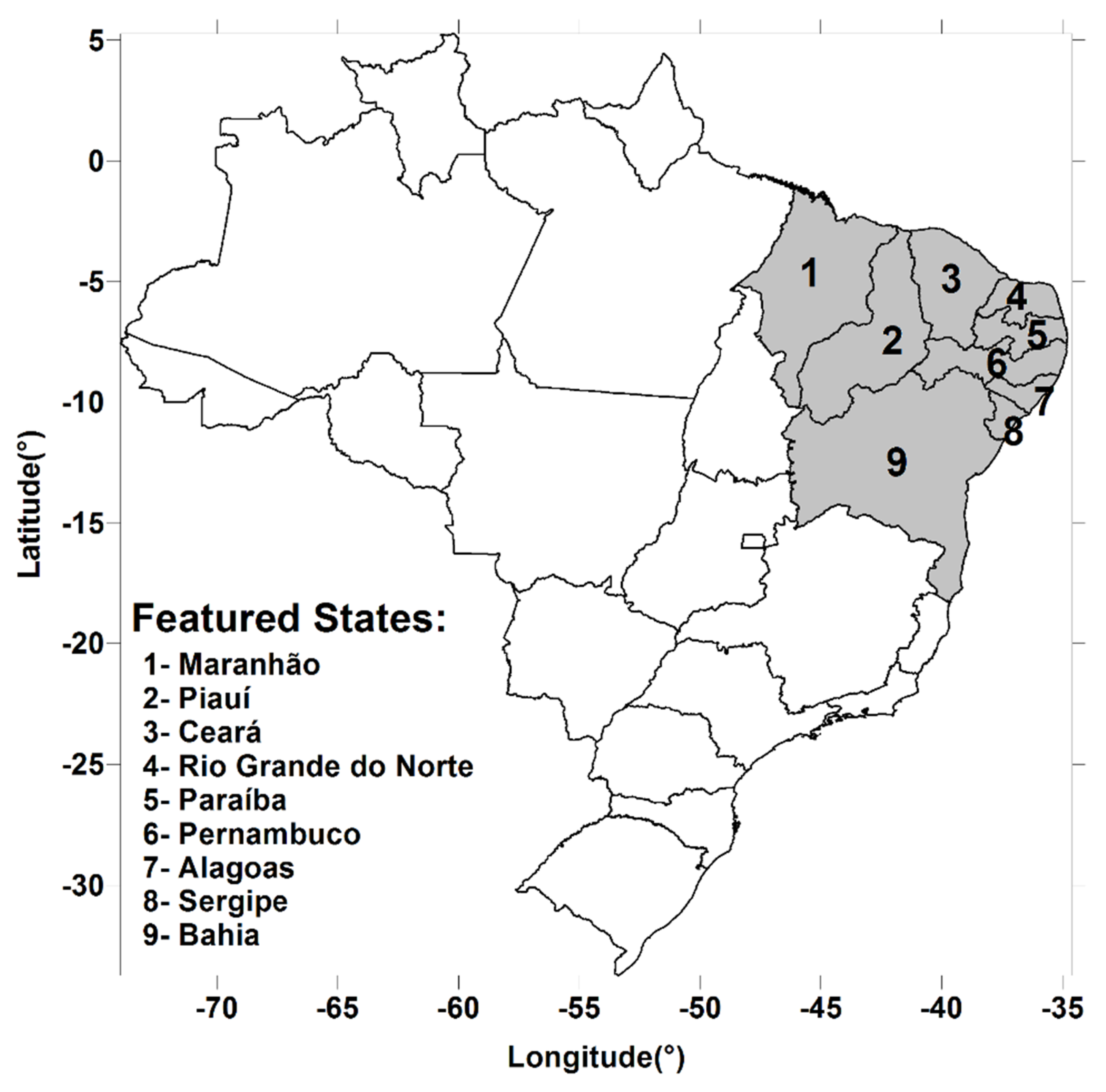
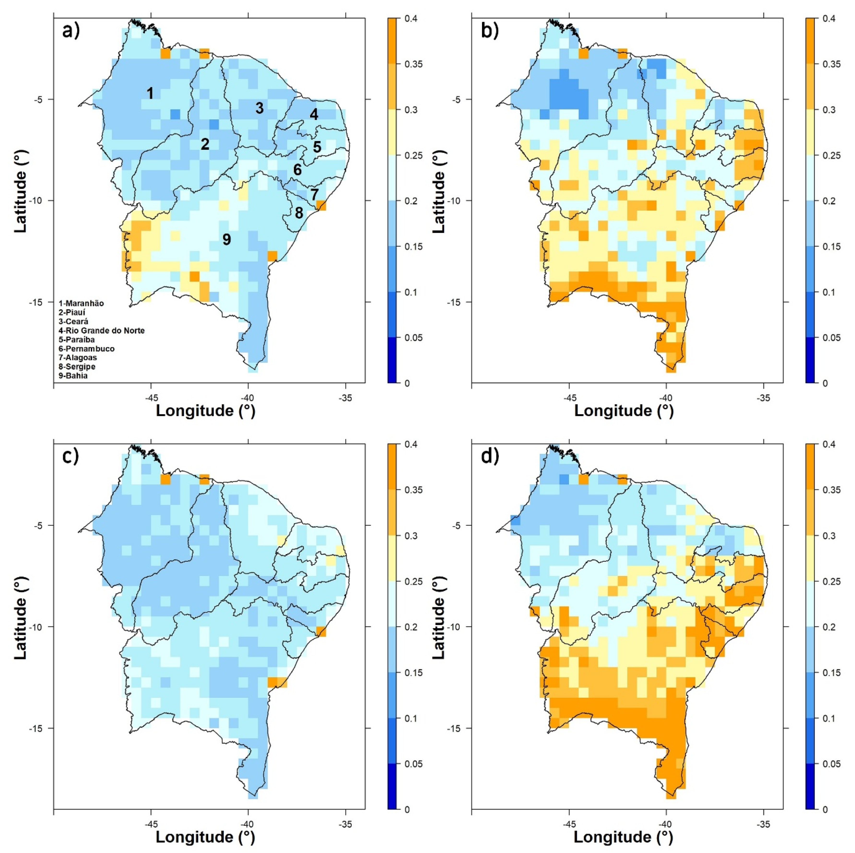
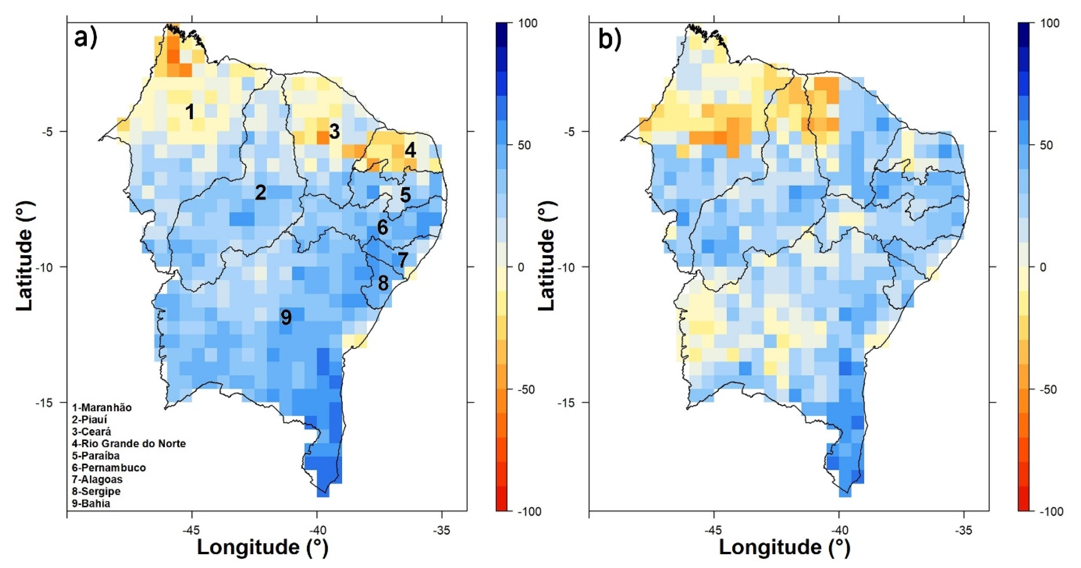
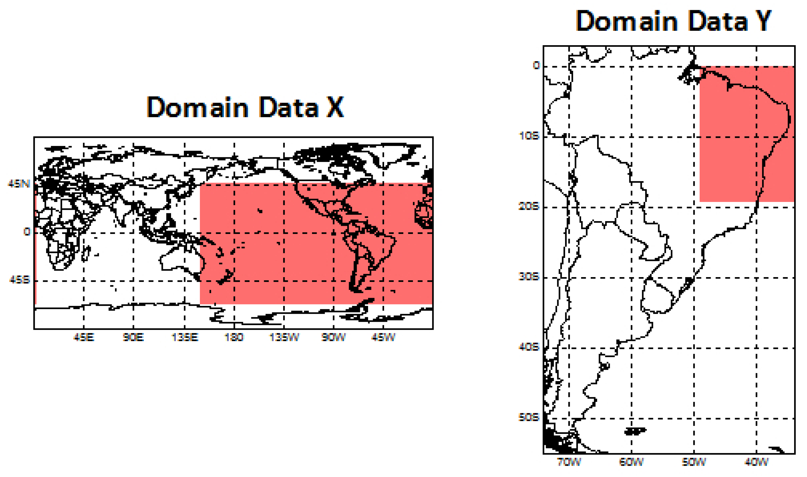
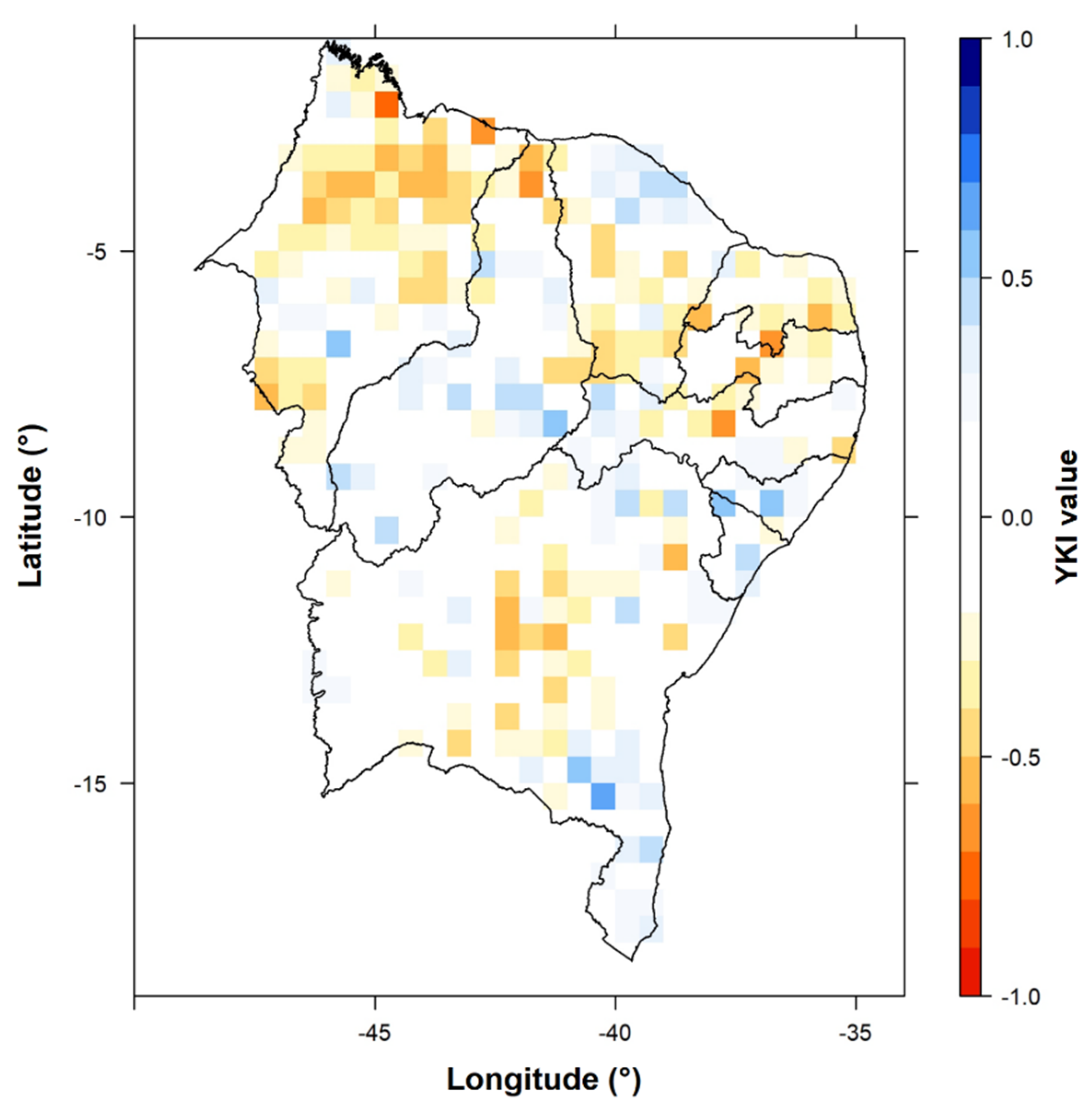
2.1. Data and Region of Study

For this work, we used an interpolated gridded monthly precipitation time series provided by the University of Delaware, with the spatial resolution of 0.5° × 0.5° for the NEB (Figure 1). Reference [46] assessed the quality of version 3 of this dataset by comparing it to control stations in Rio Grande do Norte that represent different physiographic properties. This paper uses version 4 (from www.esrl.noaa.gov/psd/data/gridded/data.UDel_AirT_Precip.html (accessed on 26 February 2019)). SST data were used as the predictor variable of the model. The data originate from the Extended Reconstructed Sea Surface Temperature (ERSST) project, version 5, which is derived from the International Comprehensive Ocean–Atmosphere Dataset (ICOADS) (from www.esrl.noaa.gov/psd/data/gridded/data.noaa.ersst.v5.html (accessed on 3 March 2019)), with a 2° × 2° resolution. Layer thickness (1000–500 mb) was also used, calculated from a geopotential height reanalysis provided by the National Center for Environmental Prediction (NCEP) Reanalysis 2, with a 2.5° × 2.5° spatial resolution (from http://www.cpc.ncep.noaa.gov/products/wesley/reanalysis2/kana/reanl2-1.htm (accessed on 3 March 2019)).

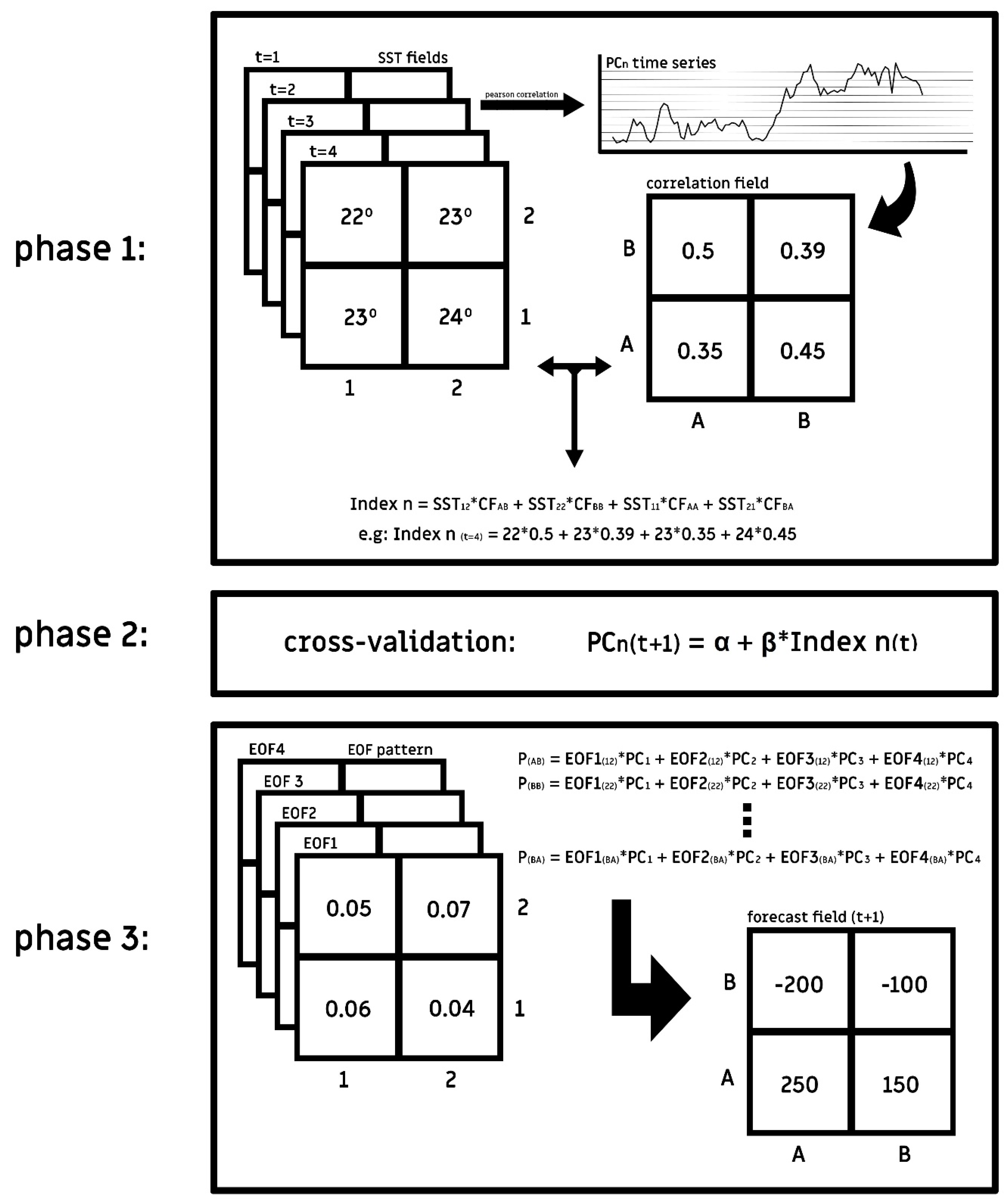
2.2. Description of the Empirical Model

The statistical model used in this study is based on the method initially proposed by [47] and subsequently implemented in [31,48,49,50]. Figure 2 illustrates a diagram with details on how the model is built. There are three main steps (phases), from tuning to validation. Phase 1 consists of an empirical process of calculating lagged SST indices that have a good correlation with the principal components (PCs) of precipitation. These indices and the PCs of precipitation are later used as predictor and predictand variables, respectively, in a linear regression model. First, the EOF technique, also known in statistics as principal component analysis (PCA) [51], is applied to the precipitation data. The technique is applied to obtain an n number of time series that concentrate most of the precipitation variability observed in the NEB (denoted as PC_n in Figure 2). Each PC is then compared to all lagged SST series in the global domain to obtain the Pearson correlation values. The outcomes of this are the correlation fields (CF) that are used to calculate the indices. This is shown in phase 1 in Figure 2, on the right. The bottom part of the phase 1 box illustrates how each index is calculated. Each grid point in the SST field has a corresponding correlation value from CF that works as a weight. The higher (lower) the correlation at a given point, the more (less) important that point is for the index. Points with statistically significant correlation lower than the 5% confidence level are set to a correlation value equal to 0. Finally, the indices are calculated by adding all the points to the CF-weighted lagged SST field, that is, for each PC in the precipitation field, a highly correlated SST index is generated.

Once the PCs of the precipitation field and the lagged SST indices for each PC are obtained, these series are used in a simple linear regression model in phase 2. The model is used to predict the next PC value using the last value of its corresponding index. In this phase, the model undergoes an adjustment and a cross-validation procedure. Thus, it is possible to obtain a hindcast of forecasts independently of the precipitation PCs.

One of the products derived from the EOF technique after it has been applied to spatial data is the spatial pattern of the modes (spatial pattern of the PCs). These patterns arise from parameters that are derived from the spatially referenced technique. It is from these parameters that the PCs are calculated in the EOF process, allowing us to couple the PCs and, therefore, to reconstruct the precipitation field. These parameters are used by combining the expected PCs to build a predicted precipitation field. This process occurs in phase 3, which is detailed in the last panel of Figure 2. The grids at the left of the phase 3 panel represent the spatial patterns of each precipitation data mode. The equations at the top of that panel show how the forecast is performed for each grid point: the product between each predicted time series (PC) and their corresponding EOF is the spatial pattern of the mode. The sum of all of these predicted spatial patterns is the model’s final precipitation forecast for the NEB.

2.3. North American Multi-Model Ensemble (NMME)

The NMME is a recent multi-agency effort to provide an operational set of forecasts of global climate models [45]. As described in [52], this project, launched in 2011, provides forecasts at global level from USA and Canada climate centers, with a uniform spatial resolution of 1° × 1°. The NMME comprises forecasts from the Climate Forecast System, version 2 (CFSv2; [53]); the Geophysical Fluid Dynamics Laboratory (GFDL [54]) and the GFDL Forecast-Oriented Low Ocean Resolution (FLOR; [55]) models; the National Center for Atmospheric Research (NCAR); the Community Climate System Model, version 4 (CCSM4; [56]); the National Aeronautics and Space Administration (NASA) and Goddard Earth Observing System, version 5 (GEOS-5), ocean data and sea ice models and data assimilation systems [57,58]; as well as two models from the Canadian Meteorological Center: the Third Generation Canadian Coupled Global Climate Model (CanCM3) and the Fourth Generation Canadian Coupled Global Climate Model (CanCM4) [59]. The NMME is the result of the integration of this set of models. The complete list of models is described in detail by [45].

We decided to use NMME outputs because several studies have revealed that the NMME’s skill outperforms forecasts of individual models [60,61,62,63]. Other works focused on assessing the NMME’s skill for specific regions and situations. For instance, there are efforts to improve seasonal climate forecasts for the African continent [64] and to predict droughts in China [65], as well as an assessment of statistical downscaling of precipitation and 2 m air temperature forecasts from the NMME for Florida, Georgia and Alabama [66].

2.4. Model Downscaling Using the Climate Predictability Tool

In this work, we did not use NMME raw data. In order to accomplish a better performance of the ensemble for the NEB, we applied a downscaling technique for post-processing the NMME’s hindcast. The technique is known as canonical correlation analysis (CCA) and is part of the climate predictability tool (CPT), which is widely used for generating operational climate predictions [67,68,69].

The CCA can be used in two ways (see Figure 1 in [15]). The first, as a purely statistical forecast model, by relating predictor variables to the predictand ones (e.g., to obtain forecasts for deviations of accumulated precipitation from SST anomalies), based on a broad hindcast period without the involvement of dynamic models [70,71,72]. The second, which is employed in the present study, relates the raw outputs of dynamic model prediction to their corresponding observations for the targeted forecast time based on a hindcast period [15]. In our case, the CCA was used to relate raw NMME forecasts of rainfall for FMA, outputted in January, to the rainfall observed in that quarter based on the hindcast period of 1982–2010.

In this process, a pre-orthogonalization is achieved by using EOF analysis separately on the model hindcasts (the X variable, or predictor) and on the corresponding observations (the Y variable, or predictand), and the set of the PC time series from these EOFs is used as input to the CCA [15,70]. This method reduces the number of variables used by the CCA, preserving the most consistent patterns of variability. The CPT applies the EOF pre-processing prior to the CCA method and then estimates the model skill using a cross-validation process [15], that is, the datasets (hindcasts) used to estimate the model skill are split in mutually exclusive subsets, so that some of them are used to make the estimates and the remaining ones are used for validation. The method of cross-validation is characterized by the aforementioned process of subsequent training and validation steps, repeating itself until every dataset has been used at some point to validate the model without having been used to train it.

Analogously to [15], the predictor domain for the NEB (Domain Data X, Figure 3, left panel) is purposely designed to be larger than the predictand region itself (Domain Data Y, Figure 3, right panel). The selected NMME predictor grid spans from 150°E to 0° in longitude and from 66° S to 48° N in latitude. The choice was motivated by the fact that the grid encompasses the domains of the main modes of climate variability that are known to affect the behavior of weather systems that, in turn, modulate the rainfall regime of the NEB. That same domain was proven to be effective in [15].

2.5. Deterministic and Probabilistic Assessment

For newly developed models aimed at climate forecasts, it is expected from the developer to perform and present assessments of the model skill from both the deterministic and probabilistic perspectives. The dexterity of the model in outputting deterministic forecasts was estimated by using the anomaly correlation coefficient (ACC) (Equation (1)), also known as the Pearson correlation coefficient, where F’ is the predicted rainfall anomaly, O’ is the observed anomaly and N is the total number of observed and predicted data that are available in the sample. For the probabilistic assessment of the model, we used the Brier score (BS) (Equation (2)), where $f_t$ is the probability of occurrence of any precipitation and $O_t$ is the current condition of the event (1 for occurrence and 0 for non-occurrence). In order to generate probabilistic forecasts, it is necessary to convert the deterministic forecast in probabilistic values, which, in turn, are derived from a probability distribution. For three-month data, a probability distribution of the Gaussian (normal) type is usually well suited to model the statistical behavior of the data. We applied the Yule–Kendall index of skewness (YKI) to verify the suitability of the series to a normal distribution. The closer to zero the YKI value is, the greater the suitability of the dataset is to a normal distribution. Figure 4 shows that, for most of the grid points of the NEB, the YKI values are equal to or very close to zero. This confirms the reasonability of applying the Gaussian distribution to these data.

As for the probabilistic forecasts, precipitation is considered below (above) the climatological normal when accumulated rainfall is lower (higher) than the 0.33 (0.66) percentile. The deterministic forecasts were converted to probabilistic ones by using logistic regression. As the NMME is the reference model in this study, we used relative metrics to assess the skill gain of one model over the other. The skill correlation score (SCS) (Equation (3)) is the metric that determines, in percentage terms, how much a model was better than the other in outputting deterministic forecasts. In Equation (3), r_forecast is the Pearson correlation value of the model that is undergoing evaluation (EmpM), and r_reference is the Pearson correlation of the reference model (NMME). For the probabilistic forecasts, we used the Brier skill score (BSS) (Equation (4)) to quantitatively assess the relative gain in skill of one model over the other. In this Equation, BS_forecast is the is the Brier score of the model under analysis (EmpM), whereas BS_ref is the Brier score of the reference model (NMME).

$$\mathrm{ACC}=\frac{\frac{1}{N}{\sum }_{i=1}^{N}F{\prime }_{i}O{\prime }_i}{\sqrt{\frac{1}{N}{\sum }_{i=1}^N{F}_i^{\prime 2}\frac{1}{N}{\sum }_{i=1}^N{O}_i^{\prime 2}}}$$

(1)

$$\mathrm{BS}=\frac{1}{N}\sum _{t=1}^N{\left(f_t-o_t\right)}^2$$

(2)

$$\mathrm{SCS}=\frac{r_{\mathrm{forecast}}-r_{\mathrm{reference}}}{1-r_{\mathrm{reference}}}\times 100$$

(3)

$$\mathrm{BSS}=1-\frac{\mathrm{BSforecast}}{{\mathrm{BS}}_{\mathrm{ref}}}\times 100$$

(4)

3. Results and Discussion

For the precipitation forecast of the FMA quarter in the NEB, we focused on the first three leading modes obtained by EOF. The choice of this number of modes was made because the general dexterity of the model tends to decay if more than three main modes are adopted, and also because they presented reasonable teleconnection patterns that are discussed in the next subsection. The first three leading modes account for 44%, 18% and 8% of the variability, respectively. Together, they represent 70% of the total dataset variability. The remaining modes were discarded, as they were regarded as noise.

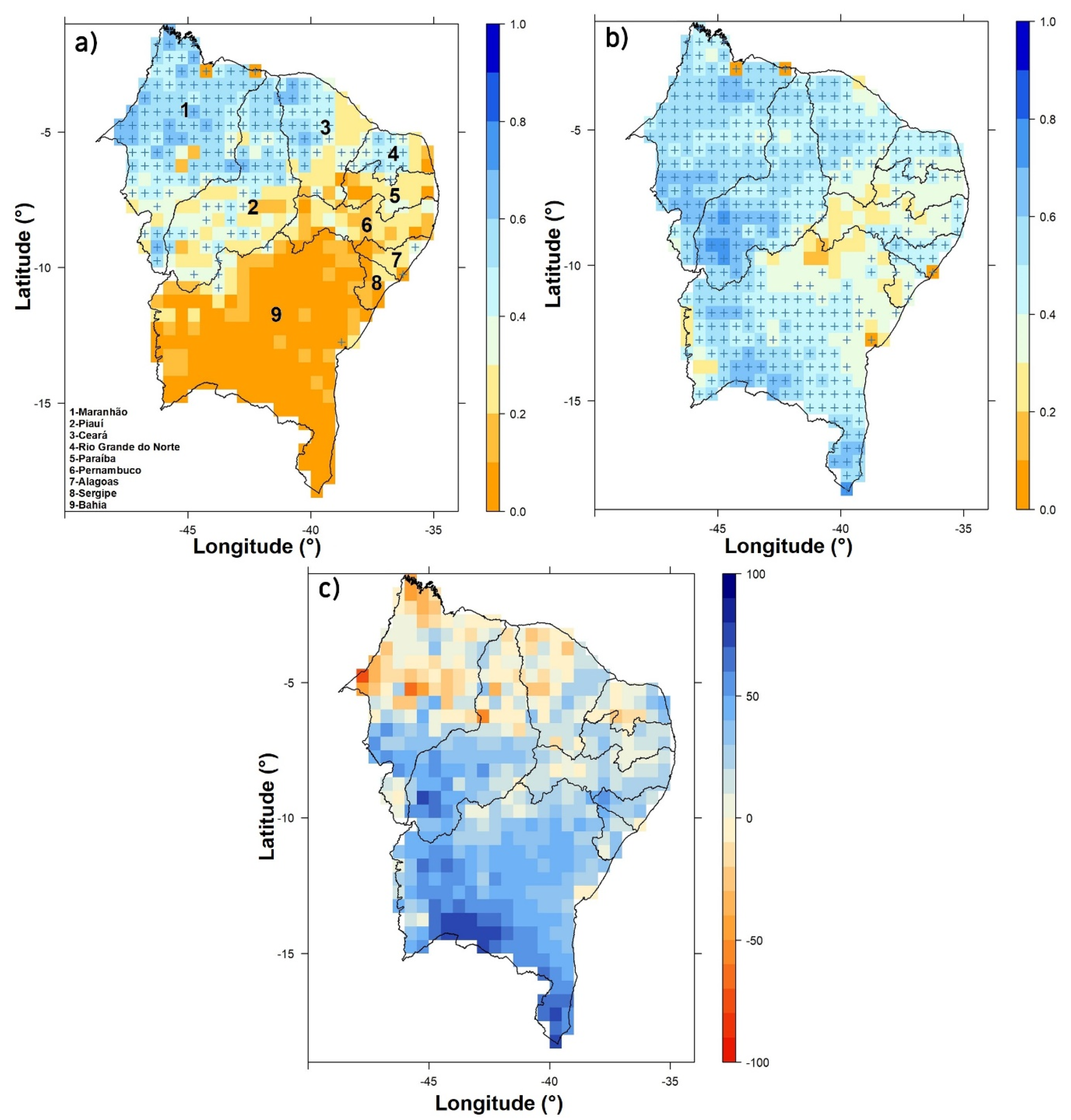
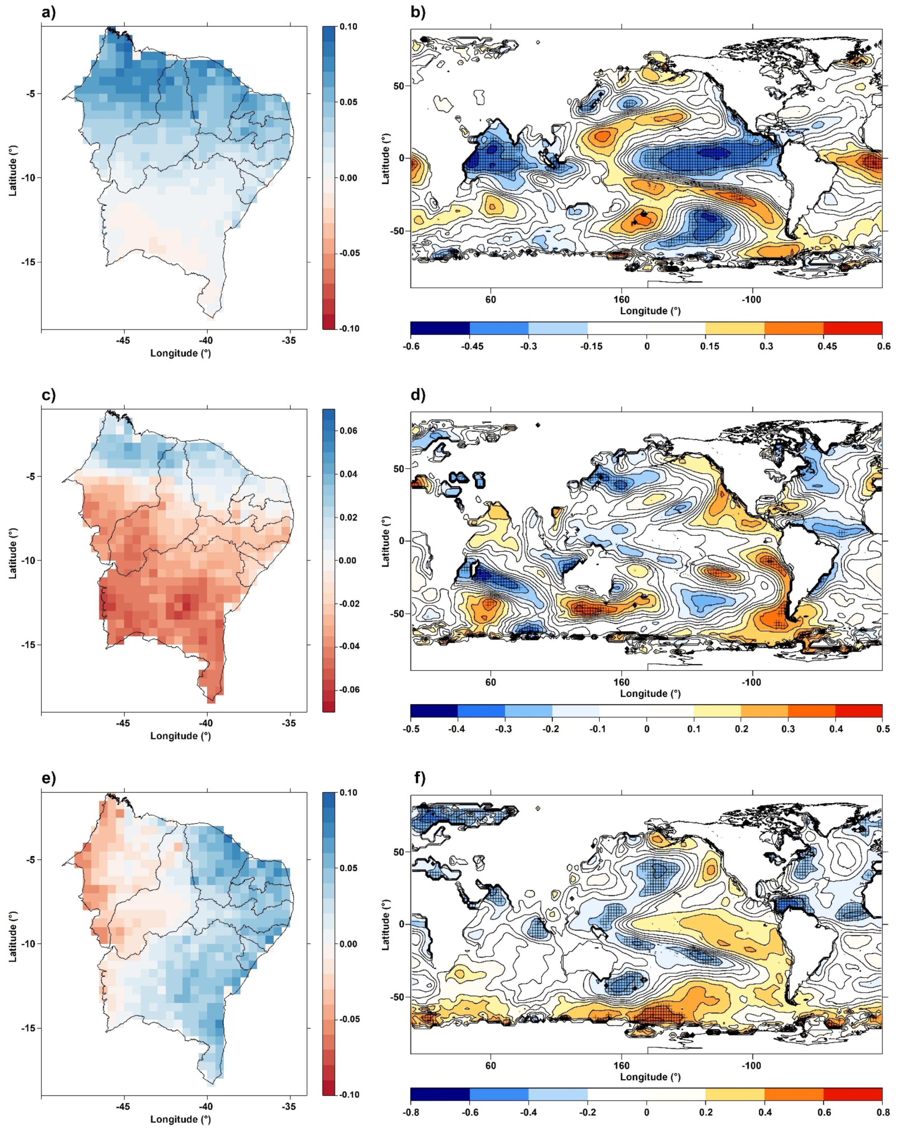
3.1. Precipitation and Teleconnection Patterns

The EOF spatial loading patterns for each of the leading modes are shown in Figure 5a,c,e, and their respective lagged SST anomalies correlation fields are shown in Figure 5b,d,f. Prior to proceeding with the teleconnection analysis presented hereinafter, it is important to clarify that negative values in the loading patterns imply correlations with SST anomalies of the opposite sign (relative to the ones presented in the scale at the bottom of Figure 5b,d,f).

The loading pattern inherent to the first leading mode is shown in Figure 5a, exhibiting a prominent concentration in the northern sector of the NEB (Figure 5a). The pattern showed a gradual decrease towards the southern sector of the NEB, with values nearing the maximum of 0.10 along the northern coast, and neutral to slightly negative in the southern half of the region. Significant negative teleconnection patterns were observed between the mode and the equatorial Pacific, most of the South Pacific and in the northwestern region of the Indian Ocean (Figure 5b). A positive teleconnection pattern was present along the equatorial Atlantic, with higher significance and prevalence of correlation coefficients higher than 0.45 around the South Atlantic tropical (SAT) region, outlined by [7] as one of the two regions chosen by them to propose their SST Atlantic dipole index. This teleconnection is coherent with results found in literature that show the influence of the Atlantic Ocean in the rainfall regime of the NEB [73,74,75]. The huge area of significant and strong negative correlation (ranging from 0.3 to 0.6) along the equatorial Pacific presented a pattern that corresponds to the ENSO domain.

Primarily, the reduction in the NEB precipitation usually observed during El Niño has been attributed to large-scale changes in the Walker circulation, causing an eastward displacement of the affecting cell, positioning its rising branch over the eastern equatorial Pacific, where abnormally warm surface waters prevail, and its sinking branch over the tropical Atlantic [76]. Such anomalies in the Walker circulation can produce subsidence over the region, which can also be affected by a strengthened and shifted sinking branch of the Hadley cell when the ITCZ is displaced northward [77,78]. However, the ENSO SST anomalies may have different effects on the tropical Atlantic depending on their spatial structure and duration [37]. Some authors use the terms “canonical” and “non-canonical” to differentiate the cases according to their observed response in the Atlantic and, consequently, in the NEB precipitation. Among them, are the authors of [37,76,79]. Canonical El Niño events exhibit their maximum anomalous warming in the eastern Pacific, which, in turn, causes a warming of the tropical North Atlantic and a cooling of the equatorial and tropical South Atlantic, leading to deficient rainfall over the NEB [79]. This interbasin connection is mainly through the changes mentioned above in the Walker circulation, which lead to an intensification of the southeast trades over the equatorial Atlantic in DJF, with the stronger southeast winds triggering upwelling equatorial Kelvin waves that cause cooling of the equatorial Atlantic in MAM [37,76]. The opposite tends to happen for canonical La Niña events [79].

Our findings are highly consistent with the teleconnection described above between the equatorial Pacific and the tropical Atlantic during canonical ENSO episodes, as the first leading mode (Figure 5a,b) exhibited, at the same time, strongly significant negative correlations with the ENSO area and positive correlations with the SAT area, as well as a slight negative correlation with the tropical North Atlantic. It is also worth noting that the teleconnection with the equatorial Pacific was stronger in, if not almost restricted to, the domains of the Niño3.4, Niño3 and Niño1+2 indices, which are areas that define the canonical ENSO events. It should be mentioned that the core of the negative correlation found here, with values exceeding 0.45, covered parts of the Niño3.4 and almost the entirety of the Niño3 regions. Furthermore, the lagged nature of the teleconnection was also present in our findings, as the SST anomaly field (Figure 5b) is built with December data.

Additionally, the effect in the Atlantic was mostly seen in the northern NEB (Figure 5a), which is precisely the region regarded as most susceptible to the latitudinal migration of the ITCZ, which, in turn, is governed by the meridional gradient of the SST anomalies in tropical Atlantic, as highlighted by [73,75,80,81,82].

Indeed, during the positive phase of the AMM, i.e., with a tropical North Atlantic warmer than the tropical South Atlantic, the descending branch of the Hadley circulation is positioned over the NEB and the adjoining tropical South Atlantic. This causes the ITCZ to fail to reach a more austral position (and, therefore, the northern NEB) during the FMA quarter [73,75,80,83,84].

Considering that the time series used in this study encompassed a total period of 29 years, it was not possible to be more assertive regarding teleconnections with oscillations of much lower frequencies. However, it is known that the ENSO and PDO climate patterns are clearly related, both spatially and temporally, to the extent that the PDO may be viewed as ENSO-like interdecadal climate variability [85], with the main difference between PDO and ENSO being their time scales, for, while the PDO phases persist for 20 to 30 years, the typical ENSO events persist for 6 to 18 months [86]. Furthermore, according to [86,87], El Niño (La Niña) events are more (less) intense and occurs in higher (lesser) number during the positive phase of the PDO, with the opposite occurring during its negative phase. Therefore, a teleconnection between the first mode and the PDO may also be hypothesized.

Regarding the second leading mode, its EOF loading pattern exhibited negative values for nearly all the NEB, to the point of exceeding 0.06 for areas in the center-south and in the southwest. The far northern region was an exception presenting low positive numbers, which were rarely above 0.03 (Figure 5c). Therefore, we focus our analysis of this mode on the southern NEB region. The teleconnection patterns with the global SST field (Figure 5f) were rather punctual, suggesting that the mode was not linked to any known major oscillations with frequencies lower than the seasonal scale. There were significant teleconnections with waters off the eastern coast of Madagascar and the southern coast of Australia, where the correlation coefficients reached about −0.5 and 0.5, respectively (Figure 5d). These regions are considered key points in Rossby wave instability, which ripples across the Pacific until it reaches South America. The correlation areas observed off the western coast of South America, with values in excess of 0.3, were also consistent with the path of Rossby wave trains that ripple through the subtropical and polar jets, as it is known that, when they reach approximately 80° W, the wave trains combine into a single wave [88].

Those waves are associated with the penetration of frontal systems in the South American continent. Eventually, these transient systems reach lower latitudes and, therefore, the southern NEB, being considered one of the most important weather systems to modulate the rainfall regime of that region [78,89,90,91], especially the state of Bahia, where the maximum EOF loading values of this mode are observed (Figure 5c). However, it should be noted that the wet season varies within the NEB, and, in this region, it is concentrated in the DJF period of the year [78,82,88,91], having only one month in common with the FMA quarter.

Still, on the possible teleconnection with higher latitudes analyzed above, in addition to the mid-latitude areas commented before, it is interesting to notice several pockets off the coast of Antarctica presenting significant correlations (Figure 5d). As recollected by the authors of [92], 20%–30% of monthly sea level pressure (SLP) variability south of 20° S is explained by the Southern Annular Mode (SAM), also known as the Antarctic Oscillation (AAO). This oscillation is considered the most significant forcing of intraseasonal to decadal climate variability in the middle- to high-latitude Southern Hemisphere [93]. Therefore, given the relevance of the southern oceans to the behavior of the frontal systems that affect South America, it is possible to conjecture a teleconnection between the southern NEB precipitation and the SAM as well.

There was also a statistically significant correlation area in the North Pacific, around Japan, that may be linked to the Kuroshio–Oyashio Extension. However, given that the inherent correlation was subtle (lower than 0.3 for most of it) and that a possible influence does not have grounds in the literature, we chose to nullify that area for this study, so that the model could technically disregard it.

The third leading mode presented a zonal gradient loading pattern, with positive values in the eastern half of the NEB and negative values in the westernmost sector (Figure 5e). Almost throughout the eastern area, the EOF values remained above 0.05. From the corresponding global SST field, it was possible to identify a significant negative teleconnection between the precipitation over the eastern NEB and the SST anomalies in the Caribbean Sea (between −0.4 and −0.6), as well as with the eastern tropical North Atlantic (Figure 5f), with the latter corresponding to the NAT index domain, and the other region defined by [7] for their aforementioned Atlantic dipole. It is useful to recall that the North Atlantic may, by itself, determine the latitudinal migration of the ITCZ, by leading the AMM [91,94]. According to these authors, during the positive phase of the NAO, the northeast trade winds, which push the ITCZ to the south during the austral summer, are enhanced. Still conforming to them, these effects, i.e., the greater vigor of the Hadley cell, its closer proximity to the NEB and the increased moisture flux from the Atlantic, eventually result in increased precipitation over the region.

Moreover, in that regard, the evident upward trend in the time series of the third mode (Figure 6c) may be linked to the Atlantic Multidecadal Oscillation (AMO), which transitioned from the negative to positive phase in the 1990s. The positive phase of the AMO naturally implies the predominance of positive phases of the NAO in shorter time scales, which, according to the above, are considered favorable to rainfall over the NEB.

It should be remarked, though, that the eastern NEB is known to have its wet season concentrated in the AMJJ period [82,87,89,91,95], not exactly the FMA quarter.

Significant correlations were also seen with the southwest of the Pacific Ocean, presenting a dipolar pattern of association, with coefficients exceeding 0.4 in the high latitudes and −0.4 in the middle latitudes. Interestingly, this pattern resembled the one identified by [78] as responsible for 39% of the variability of the South Pacific, with anomalies of opposite sign centered around 35° S, 160° W and 60° S, 130° W. Still, according to those authors, this mode is highly correlated to ENSO and the Interdecadal Pacific Oscillation (IPO), being characterized by a horseshoe structure with positive (negative) anomalies located on subtropical regions of both the North and South Pacific, and negative (positive) anomalies on the eastern tropical Pacific. That is almost exactly the correlation pattern that was observed here in Figure 5f, where a broad region of significant negative correlations formed a horseshoe shape that contoured a tropical area of positive (although not significant) correlations in the eastern tropical Pacific. Therefore, a teleconnection with this mode, called the South Pacific Ocean Dipole (SPOD) [96] was also identified.

Additionally, one of the regions that formed the horseshoe pattern mentioned above, the one presenting significant negative correlations (with values between −0.4 and −0.6) centered in the subtropical to middle latitudes of the central North Pacific, is generally used to define the PDO index [6,85].

Actually, this same pattern of SST anomalies has been described by [97] as a boomerang-shaped pattern of stronger anomalies of one sign along the equator over the central and eastern Pacific and weaker anomalies of the opposite sign over mid-latitude regions of both hemispheres; it was also described by [98] as a tripole pattern of SST anomalies in the Pacific, with three large centers of action and variations on decadal timescales, with the sign of the equatorial region being the opposite of the one in the central-west of the North Pacific and in the central-west of the South Pacific. In both cases, the authors referred to the SST anomalies pattern that characterizes the IPO. For both of them, the IPO and the PDO are closely related, highlighting the similarity between their time series and the fact that the two of them exert a low-frequency modulation of ENSO and its teleconnections. It is also suggested that the PDO can be considered as the North Pacific node of the IPO [98], or that the IPO can be a Pacific-wide manifestation of the PDO [97].

Therefore, the SST correlation pattern in Figure 5f made us infer that the upward trend in rainfall observed for our third leading mode in Figure 6c, in addition to the AMO influence discussed before, is also possibly owed to the transition from the positive to the negative phases of the IPO (and the PDO) in the end of the past century.

Similar to the correlation pattern of the second leading mode, the one associated with the third mode also exhibited several areas of correlation around the Antarctic continent, almost forming a belt of correlations of the same sign, which occasionally surpassed 0.6 (Figure 5f). Knowing that the Easterly Wave Disturbances (EWDs) are the main cause of rainfall over the eastern NEB [73,89,91,95] and that more than 70% of the occurrences of that system in the region have origins found to be associated with cold fronts [95] (which naturally originate in the high latitudes), a teleconnection of the rainfall over eastern NEB with the SAM can be inferred too.

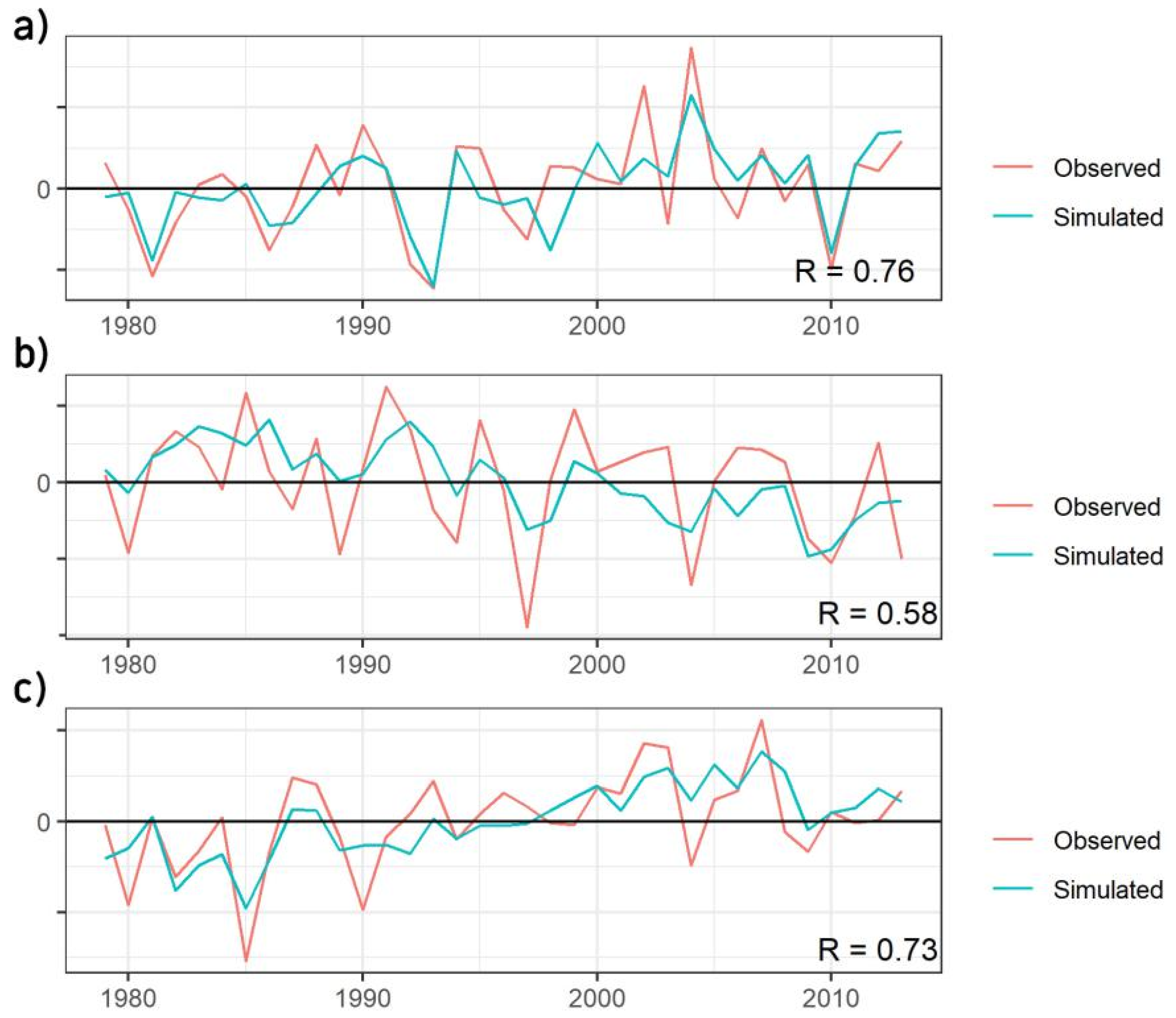
3.2. Forecasting Patterns of Precipitation Anomalies

The significant teleconnections found between each mode and the two-month lagged SST anomalies are useful for the adjustment of simple linear regression models that use the time series of each mode as the predictand, and the SST anomalies as the predictor field. Overall, the teleconnections allowed for a reasonable predictability for all the analyzed modes (Figure 6a–c). The first leading mode was linked to a variability at relatively lower frequencies (e.g., ENSO and AMM). For this reason, probably, it proved to be the most predictable mode, with a 0.76 correlation between the observed and the predicted time series. The association of the second mode with the propagation of higher frequency atmospheric waves, as discussed in the previous section, resulted in the attainment of the lowest correlation among the modes, although still satisfactory, at 0.58. The third mode presented a noticeable trend and lower variability, with both factors leading to a stability that, in turn, resulted in a fair predictability of the mode, having achieved a correlation of 0.73.

By having the ability to predict modes individually, it becomes possible to predict the spatial precipitation patterns in the NEB by the method presented in phase 3 of the diagram (Figure 2). The NMME, which represents the state-of-the-art in seasonal forecasting by general circulation models, accomplished significant performance in the northwestern part of the NEB (Figure 7a). However, for other areas within the domain, it obtained statistically non-significant results. This demonstrates a clear need to improve forecasts for the NEB, especially for its southern and eastern sectors. Conversely, the EmpM achieved significant predictability for most of the NEB (Figure 7b). The areas with higher predictability were located at the center-west and southern portions, where the spatial correlations were usually above 0.6. A region of statistically non-significant predictability spread over parts of the states of Bahia, Sergipe, Pernambuco, Paraíba and Ceará (Figure 7b). This region represents the core of the semi-arid zone.

The SCS allowed us to assess the performance of the empirical model against the performance of the NMME. It is possible to observe that the EmpM was able to consistently outperform the NMME for most of the NEB (Figure 7c), to the point of reaching 100% in the some of the southernmost areas. The average EmpM gain against NMME was of 50%. On the other hand, the NMME forecasts for the northernmost part of the NEB were overall superior to those outputted by the EmpM.

In probabilistic terms, obtaining BS values less than or equal to 0.25 means that the model has an accuracy rate higher than 50%, rendering the model superior to the referential climatology. The NMME was inefficient in a small area of the southwestern NEB in forecasts below the normal (Figure 8a) and in most of the southern area, as well as in some of the eastern coast, in forecasts above the normal (Figure 8b). The EmpM, in turn, obtained a BS value lower than 0.25 for nearly all the NEB territory under circumstances below the normal (Figure 8c). In forecasts above the normal, the model was inefficient over a broad area that encompassed the southern and most of the eastern regions (Figure 8d). Visually, the NMME was superior to the EmpM with regards to the BS parameter. Finally, we resorted to the BSS to compare once again the EmpM performance to the one of the NMME. In forecasts above the normal (Figure 9b), the pattern bore similarity to the one shown in Figure 7c, with the NMME prevailing in the northwestern region, and the EmpM showing superiority for nearly all the other areas. In forecasts below the normal (Figure 9a), the NMME was superior in a broader strip across the northern region, but the EmpM was still better for most of the NEB.

4. Conclusions

In this study, we developed and calibrated an empirical model to create seasonal forecasts for the rainy period of the NEB and compared it to an ensemble of dynamic models that represent the state-of-the-art in seasonal forecasting. The model predicts the rainfall of the FMA quarter from individual forecasts of each dominant mode of the region’s precipitation. The teleconnection analysis between the leading precipitation modes and the lagged SST field showed consistent associations that enabled the individual forecasting of each mode and, subsequently, precipitation forecasts for the NEB.

The first leading mode showed remarkable correlations with broad regions of the Pacific, Atlantic and Indian Oceans. It is widely established in the literature that the SSTs of the equatorial Pacific and the tropical Atlantic exert considerable influence on the NEB precipitation. According to the spatial pattern obtained by EOF, such influence is significantly concentrated in the northern part of the NEB, which is known to be the most susceptible to both the AMM and ENSO. Additionally, it is the region that has the FMA period for the wet season, so obtaining that particular spatial pattern for the first leading mode is substantially coherent.

The teleconnection patterns inherent to the second leading mode suggested that it may be linked to the propagation of high-frequency atmospheric waves (e.g., Rossby waves). The statistically significant correlations with the lagged SST anomalies of the South Pacific, in areas that typically nest atmospheric wave excitation, point in the direction of that hypothesis. Moreover, the loading pattern of this mode resembled a meridional dipole, with the maximum EOF loading in the southern NEB, which is precisely the sector that owes its rainfall primarily to the incursion of frontal systems. Teleconnections of this mode with SST regions of higher southern latitudes made it possible to conjecture an influence of the SAM as well.

A zonal gradient pattern was observed for the third EOF leading mode, with maximum loading in the eastern NEB. The positive teleconnections with two broad areas in the tropical North Atlantic may be owed to the influence of the NAO, as previously discussed. As for the Pacific, the horseshoe shape of the negative correlation areas resembled that of the SPOD, with one of those areas, the one centered in the North Pacific, having been identified as the PDO index domain. The remarkable upward trend noticed in the time series of this mode is probably linked to the PDO (and the IPO) or the AMO, or to both of these low-frequency modes of the Pacific and the Atlantic, respectively.

The identified teleconnection patterns were used to generate simulated time series that awee noticeably correlated with the observed time series of each mode. This allowed for a reasonable adjustment of linear regression models to predict each mode using the SST anomalies field as the predictor variable. Deterministically, the EmpM outperformed the NMME, especially in the center-south portion of the NEB, whereas the northwestern region was better forecasted by the NMME. The results were similar when the models were compared stochastically. The EmpM was better than the NMME for most of the region, especially for the center-south area. The NMME superiority was restricted to some areas spread over the northern region. From the probabilistic perspective, an overall better performance was attained by the NMME in forecasts above the normal, with the EmpM showing prevalence in circumstances below the normal.

As a future activity, we intend to apply the results obtained in this work for the calibration and verification of the Brazilian Global Atmospheric Model (BAM) [99], which is the atmospheric module of the Brazilian Earth System Model (BESM), aiming to achieve a hybrid dynamic-statistic coupling for observed surface data and to perform adjustments in the BESM seasonal forecasting for the NEB.

References

1. Dool, H.V.D. Empirical Methods in Short-Term Climate Prediction; Oxford University Press (OUP): Oxford, UK, 2006. [Google Scholar]
2. Rasmusson, E.M.; Wallace, J.M. Meteorological Aspects of the El Nino/Southern Oscillation. Science 1983, 222, 1195–1202. [Google Scholar] [CrossRef]
3. Karoly, D.F. Trend and Teleconnection Patterns in the Climatology of Extratropical Cyclones over the Southern Hemisphere. Palmen Memorial Symposium on Extratropical Cyclones; American Meteorological Society: Boston, MA, USA, 1988. [Google Scholar]
4. Gagnon, A.S.; Smoyer-Tomic, K.E.; Bush, A.B. The El Niño Southern Oscillation and malaria epidemics in South America. Int. J. Biometeorol. 2002, 46, 81–89. [Google Scholar] [CrossRef]
5. Min, S.-K.; Cai, W.; Whetton, P. Influence of climate variability on seasonal extremes over Australia. J. Geophys. Res. Atmos. 2013, 118, 643–654. [Google Scholar] [CrossRef]
6. Mantua, N.J.; Hare, S.R.; Zhang, Y.; Wallace, J.M.; Francis, R.C. A Pacific Interdecadal Climate Oscillation with Impacts on Salmon Production. Bull. Am. Meteorol. Soc. 1997, 78, 1069–1079. [Google Scholar] [CrossRef]
7. Chang, P.; Ji, L.; Li, H. A decadal climate variation in the tropical Atlantic Ocean from thermodynamic air-sea interactions. Nat. Cell Biol. 1997, 385, 516–518. [Google Scholar] [CrossRef]
8. Delworth, T.L.; Zeng, F.; Vecchi, G.A.; Yang, X.; Zhang, L.; Zhang, R. The North Atlantic Oscillation as a driver of rapid climate change in the Northern Hemisphere. Nat. Geosci. 2016, 9, 509–512. [Google Scholar] [CrossRef]
9. Hammer, G.; Hansen, J.; Phillips, J.; Mjelde, J.; Hill, H.; Love, A.; Potgieter, A. Advances in application of climate prediction in agriculture. Agric. Syst. 2001, 70, 515–553. [Google Scholar] [CrossRef]
10. Edwards, P.N. History of climate modelling. Wires Clim. Chang. 2011, 2, 128–139. [Google Scholar] [CrossRef] [Green Version]
11. Peña, M.; Chen, L.G.; van den Dool, H. Intraseasonal to Interannual Climate Variability and Prediction. In Handbook of Hydrometeorological Ensemble Forecasting; Duan, Q., Pappenberger, F., Wood, A., Cloke, H., Schaake, J., Eds.; Springer: Berlin/Heidelberg, Germany, 2019. [Google Scholar]
12. Reboita, M.S.; Dias, C.G.; Dutra, L.M.M.; Rocha, R.P.; Llopart, M. Previsão Climática Sazonal para o Brasil Obtida Através de Modelos Climáticos Globais e Regional. Rev. Bras. Meteorol. 2018, 33, 207–224. [Google Scholar] [CrossRef] [Green Version]
13. Hertig, E.; Maraun, D.; Bartholy, J.; Pongracz, R.; Vrac, M.; Mares, I.; Gutiérrez, J.M.; Wibig, J.; Casanueva, A.; Soares, P.M.M. Comparison of statistical downscaling methods with respect to extreme events over Europe: Validation results from the perfect predictor experiment of the COST Action VALUE. Int. J. Clim. 2018, 39, 3846–3867. [Google Scholar] [CrossRef]
14. Rückamp, M.; Goelzer, H.; Humbert, A. Sensitivity of Greenland ice sheet projections to spatial resolution in higher-order simulations: The Alfred Wegener Institute (AWI) contribution to ISMIP6 Greenland using the Ice-sheet and Sea-level System Model (ISSM). Cryosphere 2020, 14, 3309–3327. [Google Scholar] [CrossRef]
15. Barnston, A.G.; Tippett, M.K. Do Statistical Pattern Corrections Improve Seasonal Climate Predictions in the North American Multimodel Ensemble Models? J. Clim. 2017, 30, 8335–8355. [Google Scholar] [CrossRef]
16. Hewitson, B.C.; Crane, R.G. Consensus between GCM climate change projections with empirical downscaling: Precipitation downscaling over South Africa. Int. J. Clim. 2006, 26, 1315–1337. [Google Scholar] [CrossRef]
17. Ratnam, J.V.; Doi, T.; Behera, S. Dynamical Downscaling of SINTEX-F2v CGCM Seasonal Retrospective Austral Summer Forecasts over Australia. J. Clim. 2017, 30, 3219–3235. [Google Scholar] [CrossRef]
18. Kaspar-Ott, I.; Hertig, E.; Kaspar, S.; Pollinger, F.; Ring, C.; Paeth, H.; Jacobeit, J. Weights for general circulation models from CMIP3/CMIP5 in a statistical downscaling framework and the impact on future Mediterranean precipitation. Int. J. Clim. 2019, 39, 3639–3654. [Google Scholar] [CrossRef] [Green Version]
19. Han, Z.; Shi, Y.; Wu, J.; Xu, Y.; Zhou, B. Combined Dynamical and Statistical Downscaling for High-Resolution Projections of Multiple Climate Variables in the Beijing–Tianjin–Hebei Region of China. J. Appl. Meteorol. Clim. 2019, 58, 2387–2403. [Google Scholar] [CrossRef]
20. Ozturk, T.; Altinsoy, H.; Türkeş, M.; Kurnaz, M.; Kurnaz, L. Simulation of temperature and precipitation climatology for the Central Asia CORDEX domain using RegCM 4.0. Clim. Res. 2012, 52, 63–76. [Google Scholar] [CrossRef] [Green Version]
21. Giorgi, F.; Gutowski, W.J. Regional Dynamical Downscaling and the CORDEX Initiative. Annu. Rev. Environ. Resour. 2015, 40, 467–490. [Google Scholar] [CrossRef]
22. Bhatla, R.; Ghosh, S.; Mandal, B.; Mall, R.; Sharma, K. Simulation of Indian summer monsoon onset with different parameterization convection schemes of RegCM-4.3. Atmos. Res. 2016, 176–177, 10–18. [Google Scholar] [CrossRef]
23. Manzanas, R.; Gutiérrez, J.M.; Fernández, J.; Van Meijgaard, E.; Calmanti, S.; Magariño, M.E.; Cofiño, A.S.; Herrera, A. Dynamical and statistical downscaling of seasonal temperature forecasts in europe: Added value for sectorial applications. Clim. Serv. 2018, 9, 72–85. [Google Scholar] [CrossRef]
24. Nikulin, G.; Lennard, C.; Dosio, A.; Kjellström, E.; Chen, Y.; Hänsler, A.; Kupiainen, M.; Laprise, R.; Mariotti, L.; Maule, C.F.; et al. The effects of 1.5 and 2 degrees of global warming on Africa in the CORDEX ensemble. Environ. Res. Lett. 2018, 13, 065003. [Google Scholar] [CrossRef]
25. Giorgi, F. Thirty Years of Regional Climate Modeling: Where Are We and Where Are We Going next? J. Geophys. Res. Atmos. 2019, 124, 5696–5723. [Google Scholar] [CrossRef] [Green Version]
26. Tapiador, F.J.; Navarro, A.; Moreno, R.; Sánchez, J.L.; García-Ortega, E. Regional climate models: 30 years of dynamical downscaling. Atmos. Res. 2020, 235, 104785. [Google Scholar] [CrossRef]
27. Imada, Y.; Kanae, S.; Kimoto, M.; Watanabe, M.; Ishii, M. Predictability of Persistent Thailand Rainfall during the Mature Monsoon Season in 2011 Using Statistical Downscaling of CGCM Seasonal Prediction. Mon. Weather Rev. 2015, 143, 1166–1178. [Google Scholar] [CrossRef]
28. Chu, J.-L.; Kang, H.; Tam, C.-Y.; Park, C.-K.; Chen, C.-T. Seasonal forecast for local precipitation over northern Taiwan using statistical downscaling. J. Geophys. Res. Space Phys. 2008, 113. [Google Scholar] [CrossRef] [Green Version]
29. Kang, I.-S.; Lee, J.-Y.; Park, C.-K. Potential Predictability of Summer Mean Precipitation in a Dynamical Seasonal Prediction System with Systematic Error Correction. J. Clim. 2004, 17, 834–844. [Google Scholar] [CrossRef]
30. Kang, H.; An, K.-H.; Park, C.-K.; Solis, A.L.S.; Stitthichivapak, K. Multimodel output statistical downscaling prediction of precipitation in the Philippines and Thailand. Geophys. Res. Lett. 2007, 34. [Google Scholar] [CrossRef]
31. Xing, W.; Wang, B.; Yim, S.-Y. Long-Lead Seasonal Prediction of China Summer Rainfall Using an EOF–PLS Regression-Based Methodology. J. Clim. 2016, 29, 1783–1796. [Google Scholar] [CrossRef]
32. Madadgar, S.; AghaKouchak, A.; Shukla, S.; Wood, A.W.; Cheng, L.; Hsu, K.; Svoboda, M. A Hybrid Statistical-Dynamical Drought Prediction Framework: Application to the Southwestern United States. Water Resour. Res. 2016, 52, 5095–5110. [Google Scholar] [CrossRef] [Green Version]
33. Liu, L.; Ning, L.; Liu, J.; Yan, M.; Sun, W. Prediction of summer extreme precipitation over the middle and lower reaches of the Yangtze River basin. Int. J. Clim. 2019, 39, 375–383. [Google Scholar] [CrossRef] [Green Version]
34. Júnior, R.L.D.R.; Silva, F.D.D.S.; Costa, R.L.; Gomes, H.B.; Herdies, D.L.; Silva, V.D.P.R.D.; Xavier, A.C. Analysis of the Space–Temporal Trends of Wet Conditions in the Different Rainy Seasons of Brazilian Northeast by Quantile Regression and Bootstrap Test. Geosciences 2019, 9, 457. [Google Scholar] [CrossRef] [Green Version]
35. Júnior, R.L.D.R.; Silva, F.D.D.S.; Costa, R.L.; Gomes, H.B.; Pinto, D.D.C.; Herdies, D.L. Bivariate Assessment of Drought Return Periods and Frequency in Brazilian Northeast Using Joint Distribution by Copula Method. Geosciences 2020, 10, 135. [Google Scholar] [CrossRef] [Green Version]
36. Silva, V.B.S.; Kousky, V.E.; Silva, F.D.S.; Salvador, M.A.; Aravequia, J.A. The 2012 severe drought over Northeast Brazil. Bull. Am. Meteorol. Soc. 2013, 94, 162. [Google Scholar]
37. Rodrigues, R.R.; Haarsma, R.J.; Campos, E.J.D.; Ambrizzi, T. The Impacts of Inter–El Niño Variability on the Tropical Atlantic and Northeast Brazil Climate. J. Clim. 2011, 24, 3402–3422. [Google Scholar] [CrossRef] [Green Version]
38. Coelho, C.A.S.; Stephenson, D.B.; Balmaseda, M.; Doblas-Reyes, F.J.; Van Oldenborgh, G.J.; Doblas-Reyes, F. Toward an Integrated Seasonal Forecasting System for South America. J. Clim. 2006, 19, 3704–3721. [Google Scholar] [CrossRef] [Green Version]
39. Osman, M.; Vera, C.; Doblas-Reyes, F. Predictability of the tropospheric circulation in the Southern Hemisphere from CHFP models. Clim. Dyn. 2016, 46, 2423–2434. [Google Scholar] [CrossRef]
40. Reboita, M.S.; da Rocha, R.P.; de Souza, M.R.; Llopart, M. Extratropical cyclones over the southwestern South Atlantic Ocean: HadGEM2-ES and RegCM4 projections. Int. J. Climatol. 2018, 38, 2866–2879. [Google Scholar] [CrossRef]
41. Alves, J.M.B.; Costa, A.A.; Sombra, S.S.; Campos, J.N.B.; Souza Filho, F.A.; Martins, E.S.P.R.; Silva, E.M.; Santos, A.C.S.; Barbosa, H.A.; Melcíades, W.L.B.; et al. Um Estudo Inter-Comparativo de Previsão Sazonal Estatística-Dinâmica de Precipitação para o Nordeste do Brasil. Rev. Bras. Meteorol. 2007, 24, 20–29. [Google Scholar]
42. Lucio, P.S.; Silva, F.D.D.S.; Fortes, L.T.G.; Dos Santos, L.A.R.; Ferreira, D.B.; Salvador, M.D.A.; Balbino, H.T.; Sarmanho, G.F.; Dos Santos, L.S.F.C.; Lucas, E.W.M.; et al. Um modelo estocástico combinado de previsão sazonal para a precipitação no Brasil. Rev. Bras. Meteorol. 2010, 25, 70–87. [Google Scholar] [CrossRef]
43. Coelho, C.A.S.; Stephenson, D.B.; Doblas-Reyes, F.J.; Balmaseda, M. The skill of empirical and combined/calibrated coupled multi-model South American seasonal predictions during ENSO. Adv. Geosci. 2006, 6, 51–55. [Google Scholar] [CrossRef] [Green Version]
44. Lemos, M.C.; Finan, T.J.; Fox, R.W.; Nelson, D.R.; Tucker, J. The Use of Seasonal Climate Forecasting in Policymaking: Lessons from Northeast Brazil. Clim. Chang. 2002, 55, 479–507. [Google Scholar] [CrossRef]
45. Kirtman, B.P.; Min, D.; Infanti, J.M.; Kinter, J.L.; Paolino, D.A.; Zhang, Q.; Van Den Dool, H.; Saha, S.; Mendez, M.P.; Becker, E.; et al. The North American multimodel ensemble: Phase-1 seasonal-to-interannual prediction; phase-2 toward developing intraseasonal prediction. Bull. Am. Meteorol. Soc. 2014, 95, 585–601. [Google Scholar] [CrossRef]
46. Santos e Silva, C.M.; Lucio, P.S.; Spyrides, M.H.C. Distribuição espacial da precipitação sobre o Rio Grande do Norte: Estimativas via satélites e medidas por pluviômetros. Rev. Bras. Meteorol. 2012, 27, 337–346. [Google Scholar] [CrossRef] [Green Version]
47. Wang, B.; Lee, J.Y.; Kang, I.S.; Shukla, J.; Hameed, S.N.; Park, C.K. Coupled predictability of seasonal tropical precipitation. CLIVAR Exch. 2007, 12, 17–18. [Google Scholar]
48. Xing, W.; Wang, B.; Yim, S.-Y. Peak-summer East Asian rainfall predictability and prediction part I: Southeast Asia. Clim. Dyn. 2014, 47, 1–13. [Google Scholar] [CrossRef]
49. Yim, S.-Y.; Wang, B.; Xing, W. Prediction of early summer rainfall over South China by a physical-empirical model. Clim. Dyn. 2014, 43, 1883–1891. [Google Scholar] [CrossRef]
50. Wang, B.; Lee, J.-Y.; Xiang, B. Asian summer monsoon rainfall predictability: A predictable mode analysis. Clim. Dyn. 2015, 44, 61–74. [Google Scholar] [CrossRef] [Green Version]
51. Wilks, D.S. Statistical Methods in The Atmospheric Sciences, 3rd ed.; Academic Press: Cambridge, MA, USA, 2011. [Google Scholar]
52. Bolinger, R.A.; Gronewold, A.D.; Kompoltowicz, K.; Fry, L.M. Application of the NMME in the Development of a New Regional Seasonal Climate Forecast Tool. Bull. Am. Meteorol. Soc. 2017, 98, 555–564. [Google Scholar] [CrossRef]
53. Saha, S.; Moorthi, S.; Wu, X.; Wang, J.; Nadiga, S.; Tripp, P.; Behringer, D.; Hou, Y.-T.; Chuang, H.-Y.; Iredell, M.; et al. The NCEP Climate Forecast System Version 2. J. Clim. 2014, 27, 2185–2208. [Google Scholar] [CrossRef]
54. Zhang, S.; Harrison, M.J.; Rosati, A.; Wittenberg, A. System Design and Evaluation of Coupled Ensemble Data Assimilation for Global Oceanic Climate Studies. Mon. Weather Rev. 2007, 135, 3541–3564. [Google Scholar] [CrossRef] [Green Version]
55. Jia, L.; Yang, X.; Vecchi, G.; Gudgel, R.G.; Delworth, T.; Rosati, A.; Stern, W.F.; Wittenberg, A.T.; Krishnamurthy, L.; Zhang, S.; et al. Improved Seasonal Prediction of Temperature and Precipitation over Land in a High-Resolution GFDL Climate Model. J. Clim. 2015, 28, 2044–2062. [Google Scholar] [CrossRef]
56. Gent, P.R.; Danabasoglu, G.; Donner, L.J.; Holland, M.M.; Hunke, E.C.; Jayne, S.; Lawrence, D.; Neale, R.B.; Rasch, P.J.; Vertenstein, M.; et al. The Community Climate System Model Version 4. J. Clim. 2011, 24, 4973–4991. [Google Scholar] [CrossRef]
57. Vernieres, G.; Rienecker, M.M.; Kovach, R.; Keppenne, C. The GEOS-iODAS: Description and Evaluation; Tech. Rep. TM-2012-104606; NASA, National Aeronautics and Space Administration Goddard Space Flight Center: Greenbelt, MD, USA, 2012.
58. Borovikov, A.; Cullather, R.; Kovach, R.; Marshak, J.; Vernieres, G.; Vikhliaev, Y.; Zhao, B.; Li, Z. GEOS-5 seasonal forecast system. Clim. Dyn. 2017, 53, 7335–7361. [Google Scholar] [CrossRef]
59. Merryfield, W.J.; Lee, W.-S.; Boer, G.J.; Kharin, V.V.; Scinocca, J.F.; Flato, G.M.; Ajayamohan, R.S.; Fyfe, J.C.; Tang, Y.; Polavarapu, S. The Canadian Seasonal to Interannual Prediction System. Part I: Models and Initialization. Mon. Weather Rev. 2013, 141, 2910–2945. [Google Scholar] [CrossRef]
60. Becker, E.; Dool, H.V.D.; Zhang, Q. Predictability and Forecast Skill in NMME. J. Clim. 2014, 27, 5891–5906. [Google Scholar] [CrossRef]
61. Mo, K.C.; Lettenmaier, D.P. Objective Drought Classification Using Multiple Land Surface Models. J. Hydrometeorol. 2014, 15, 990–1010. [Google Scholar] [CrossRef]
62. Mo, K.C.; Lyon, B. Global Meteorological Drought Prediction Using the North American Multi-Model Ensemble. J. Hydrometeorol. 2015, 16, 1409–1424. [Google Scholar] [CrossRef]
63. Wood, E.F.; Schubert, S.D.; Wood, A.; Peters-Lidard, C.D.; Mo, K.C.; Mariotti, A.; Pulwarty, R.S. Prospects for Advancing Drought Understanding, Monitoring, and Prediction. J. Hydrometeorol. 2015, 16, 1636–1657. [Google Scholar] [CrossRef]
64. Thiaw, W.M.; Kumar, V.B. NOAA’s African Desk: Twenty Years of Developing Capacity in Weather and Climate Forecasting in Africa. Bull. Am. Meteorol. Soc. 2015, 96, 737–753. [Google Scholar] [CrossRef]
65. Ma, F.; Yuan, X.; Ye, A. Seasonal drought predictability and forecast skill over China. J. Geophys. Res. Atmos. 2015, 120, 8264–8275. [Google Scholar] [CrossRef]
66. Tian, D.; Martinez, C.J.; Graham, W.D.; Hwang, S. Statistical Downscaling Multimodel Forecasts for Seasonal Precipitation and Surface Temperature over the Southeastern United States. J. Clim. 2014, 27, 8384–8411. [Google Scholar] [CrossRef]
67. Climate Predictability Tool version 15.5.10; Mason, S.J.; Tippett, M.K. (Eds.) Columbia University Academic Commons: New York, NY, USA, 2017. [Google Scholar] [CrossRef]
68. Esquivel, A.; Llanos-Herrera, L.; Agudelo, D.; Prager, S.D.; Fernandes, K.; Rojas, A.; Valencia, J.J.; Ramirez-Villegas, J. Predictability of seasonal precipitation across major crop growing areas in Colombia. Clim. Serv. 2018, 12, 36–47. [Google Scholar] [CrossRef]
69. Hossain, M.Z.; Azad, M.A.K.; Karmakar, S.; Mondal, M.N.I.; Das, M.; Rahman, M.M.; Haque, M.A. Assessment of Better Prediction of Seasonal Rainfall by Climate Predictability Tool Using Global Sea Surface Temperature in Bangladesh. Asian J. Adv. Res. Rep. 2019, 4, 1–13. [Google Scholar] [CrossRef]
70. Barnett, T.P.; Preisendorfer, R. Origins and Levels of Monthly and Seasonal Forecast Skill for United States Surface Air Temperatures Determined by Canonical Correlation Analysis. Mon. Weather Rev. 1987, 115, 1825–1850. [Google Scholar] [CrossRef] [Green Version]
71. Barnston, A.G. Linear Statistical Short-Term Climate Predictive Skill in the Northern Hemisphere. J. Clim. 1994, 7, 1513–1564. [Google Scholar] [CrossRef] [Green Version]
72. Johansson, Å.; Barnston, A.; Saha, S.; van den Dool, H. On the Level and Origin of Seasonal Forecast Skill in Northern Europe. J. Atmos. Sci. 1998, 55, 103–127. [Google Scholar] [CrossRef]
73. Moura, A.D.; Shukla, J. On the Dynamics of Droughts in Northeast Brazil: Observations, Theory and Numerical Experiments with a General Circulation Model. J. Atmos. Sci. 1981, 38, 2653–2675. [Google Scholar] [CrossRef] [Green Version]
74. Chiang, J.C.H.; Kushnir, Y.; Zebiak, S.E. Interdecadal changes in eastern Pacific ITCZ variability and its influence on the Atlantic ITCZ. Geophys. Res. Lett. 2000, 27, 3687–3690. [Google Scholar] [CrossRef] [Green Version]
75. Hounsou-Gbo, G.A.; Servain, J.; Araujo, M.; Martins, E.S.; Bourlès, B.; Caniaux, G. Oceanic Indices for Forecasting Seasonal Rainfall over the Northern Part of Brazilian Northeast. Am. J. Clim. Chang. 2016, 05, 261–274. [Google Scholar] [CrossRef] [Green Version]
76. Kayano, M.T.; Andreoli, R.V. Relationships between rainfall anomalies over northeastern Brazil and the El Niño–Southern Oscillation. J. Geophys. Res. Space Phys. 2006, 111, 13101. [Google Scholar] [CrossRef] [Green Version]
77. Nobre, C.A.; Molion, L.C.B. The Climatology of Droughts and Drought Prediction. In Impacts of Climatic Variations on Agriculture. Volume 2: Assessements in Semi-Arid Regions; Parry, M.P., Carter, T.R., Konijn, N.T., Eds.; D. Reidel Pub. Co.: Dordrecht, The Netherlands, 1988; 764p. [Google Scholar]
78. Chaves, R.R.; Cavalcanti, I.F.A. Atmospheric Circulation Features Associated with Rainfall Variability over Southern Northeast Brazil. Mon. Weather Rev. 2001, 129, 2614–2626. [Google Scholar] [CrossRef] [Green Version]
79. Rodrigues, R.R.; McPhaden, M.J. Why did the 2011-2012 La Niña cause a severe drought in the Brazilian Northeast? Geophys. Res. Lett. 2014, 41, 1012–1018. [Google Scholar] [CrossRef]
80. Andreoli, R.V.; Kayano, M.T. A importância relativa do atlântico tropical sul e pacífico leste na variabilidade de precipitação do Nordeste do Brasil. Rev. Bras. Meteorol. 2007, 22, 63–74. [Google Scholar] [CrossRef]
81. Uvo, C.B.; Repelli, C.A.; Zebiak, S.E.; Kushnir, Y. The Relationships between Tropical Pacific and Atlantic SST and Northeast Brazil Monthly Precipitation. J. Clim. 1998, 11, 551–562. [Google Scholar] [CrossRef]
82. Molion, L.C.B.; Bernardo, S.O. Uma revisão da dinâmica das chuvas no Nordeste Brasileiro. Rev. Bras. Meteorol. 2002, 17, 1–10. [Google Scholar]
83. Walker, G.T. Ceará (Brazil) famines and the general air movement. Beitr. Phys. Frein. Atmosph. 1928, 14, 88–93. [Google Scholar]
84. Alvarez, M.S.; Vera, C.; Kiladis, G.N.; Liebmann, B. Influence of the Madden Julian Oscillation on precipitation and surface air temperature in South America. Clim. Dyn. 2016, 46, 245–262. [Google Scholar] [CrossRef]
85. Mantua, N.J.; Hare, S.R. The Pacific Decadal Oscillation. J. Oceanogr. 2002, 58, 35–44. [Google Scholar] [CrossRef]
86. Andreoli, R.V.; Kayano, M.T. Multi-scale variability of the sea surface temperature in the Tropical Atlantic. J. Geophys. Res. 2004, 109, 1–12. [Google Scholar] [CrossRef] [Green Version]
87. Oliveira, P.T.; e Silva, C.M.S.; Lima, K.C. Climatology and trend analysis of extreme precipitation in subregions of Northeast Brazil. Theor. Appl. Clim. 2017, 130, 77–90. [Google Scholar] [CrossRef]
88. Müller, G.V.; Ambrizzi, T. Teleconnection patterns and Rossby wave propagation associated to generalized frosts over southern South America. Clim. Dyn. 2007, 29, 633–645. [Google Scholar] [CrossRef]
89. Gomes, H.B.; Ambrizzi, T.; Herdies, D.L.; Hodges, K.; Da Silva, B.F.P. Easterly Wave Disturbances over Northeast Brazil: An Observational Analysis. Adv. Meteorol. 2015, 2015, 176238. [Google Scholar] [CrossRef] [Green Version]
90. Fedorova, N.; Levit, V.; da Cruz, C.D. On Frontal Zone Analysis in the Tropical Region of the Northeast Brazil. Pure Appl. Geophys. 2016, 173, 1403–1421. [Google Scholar] [CrossRef]
91. Costa, D.D.; Uvo, C.B.; Da Paz, A.R.; Carvalho, F.O.; Fragoso, C.R., Jr. Long-term relationships between climate oscillation and basin-scale hydrological variability during rainy season in eastern Northeast Brazil. Hydrol. Sci. J. 2018, 63, 1636–1652. [Google Scholar] [CrossRef] [Green Version]
92. Zhang, Z.; Uotila, P.; Stössel, A.; Vihma, T.; Liu, H.; Zhong, Y. Seasonal southern hemisphere multi-variable reflection of the southern annular mode in atmosphere and ocean reanalyses. Clim. Dyn. 2018, 50, 1451–1470. [Google Scholar] [CrossRef]
93. Visbeck, M. A Station-Based Southern Annular Mode Index from 1884 to 2005. J. Clim. 2009, 22, 940–950. [Google Scholar] [CrossRef] [Green Version]
94. Namias, J. Influence of northern hemisphere general circulation on drought in northeast Brazil. Tellus 1972, 24, 336–343. [Google Scholar] [CrossRef]
95. Gomes, H.B.; Ambrizzi, T.; Da Silva, B.F.P.; Hodges, K.; Dias, P.L.S.; Herdies, D.; Silva, M.C.L.; Gomes, H.B. Climatology of easterly wave disturbances over the tropical South Atlantic. Clim. Dyn. 2019, 53, 1393–1411. [Google Scholar] [CrossRef] [Green Version]
96. Saurral, R.I.; Doblas-Reyes, F.J.; García-Serrano, J. Observed modes of sea surface temperature variability in the South Pacific region. Clim. Dyn. 2018, 50, 1129–1143. [Google Scholar] [CrossRef]
97. Salinger, M.J.; Renwick, J.A.; Mullan, A.B. Interdecadal Pacific Oscillation and South Pacific climate. Int. J. Clim. 2001, 21, 1705–1721. [Google Scholar] [CrossRef]
98. Henley, B.J.; Gergis, J.; Karoly, D.J.; Power, S.B.; Kennedy, J.J.; Folland, C.K. A Tripole Index for the Interdecadal Pacific Oscillation. Clim. Dyn. 2015, 45, 3077–3090. [Google Scholar] [CrossRef]
99. Figueroa, S.N.; Bonatti, J.P.; Kubota, P.Y.; Grell, G.A.; Morrison, H.; Barros, S.R.M.; Fernandez, J.P.R.; Ramirez, E.; Siqueira, L.; Luzia, G.; et al. The Brazilian Global Atmospheric Model (BAM): Performance for Tropical Rainfall Forecasting and Sensitivity to Convective Scheme and Horizontal Resolution. Weather Forecast. 2016, 31, 1547–1572. [Google Scholar] [CrossRef]
Figure 1. Map of Brazil highlighting the Northeast region in gray, showing its labeled and identified states.
Water 13 01613 g001
Figure 2. Explanatory diagram of the adjustment, validation and forecast phases of the model.
Water 13 01613 g002
Figure 3. CCA areas for the predictor X (left) and the predictand Y (right) domains (adapted from Figure 1 by [15]).
Water 13 01613 g003
Figure 4. Yule–Kendall skewness statistics for precipitation anomaly data of the FMA quarter (1982–2010).
Water 13 01613 g004
Figure 5. The EOF loading pattern of the first, second and third leading modes obtained from their FMA precipitation (a,c,e, respectively) and their corresponding December SST correlation fields (b,d,f, respectively). The points on the map represent statistical significance at the 5% level using the student’s t-test.
Water 13 01613 g005
Figure 6. Observed and predicted time series for the first (a), second (b) and third (c) leading modes.
Water 13 01613 g006
Figure 7. Spatial correlation of the observed time series with the NMME (a) and with the EmpM (b), as well as the skill correlation score (SCS) of the EmpM against the NMME (c). The points on the map represent statistical significance at the 5% level using the student’s t-test.
Water 13 01613 g007
Figure 8. Brier score (BS) for forecasts below (left) an above (right) the normal for the NMME (a,b) and the EmpM (c,d).
Water 13 01613 g008
Figure 9. Brier skill score (BSS) for values below (a) and above (b) the normal for the EmpM in relation to the NMME.
Water 13 01613 g009
Publisher’s Note: MDPI stays neutral with regard to jurisdictional claims in published maps and institutional affiliations.