
Arsenic in Petroleum-Contaminated Groundwater near Bemidji, Minnesota Is Predicted to Persist for Centuries

 ,
,
Abstract
1. Introduction
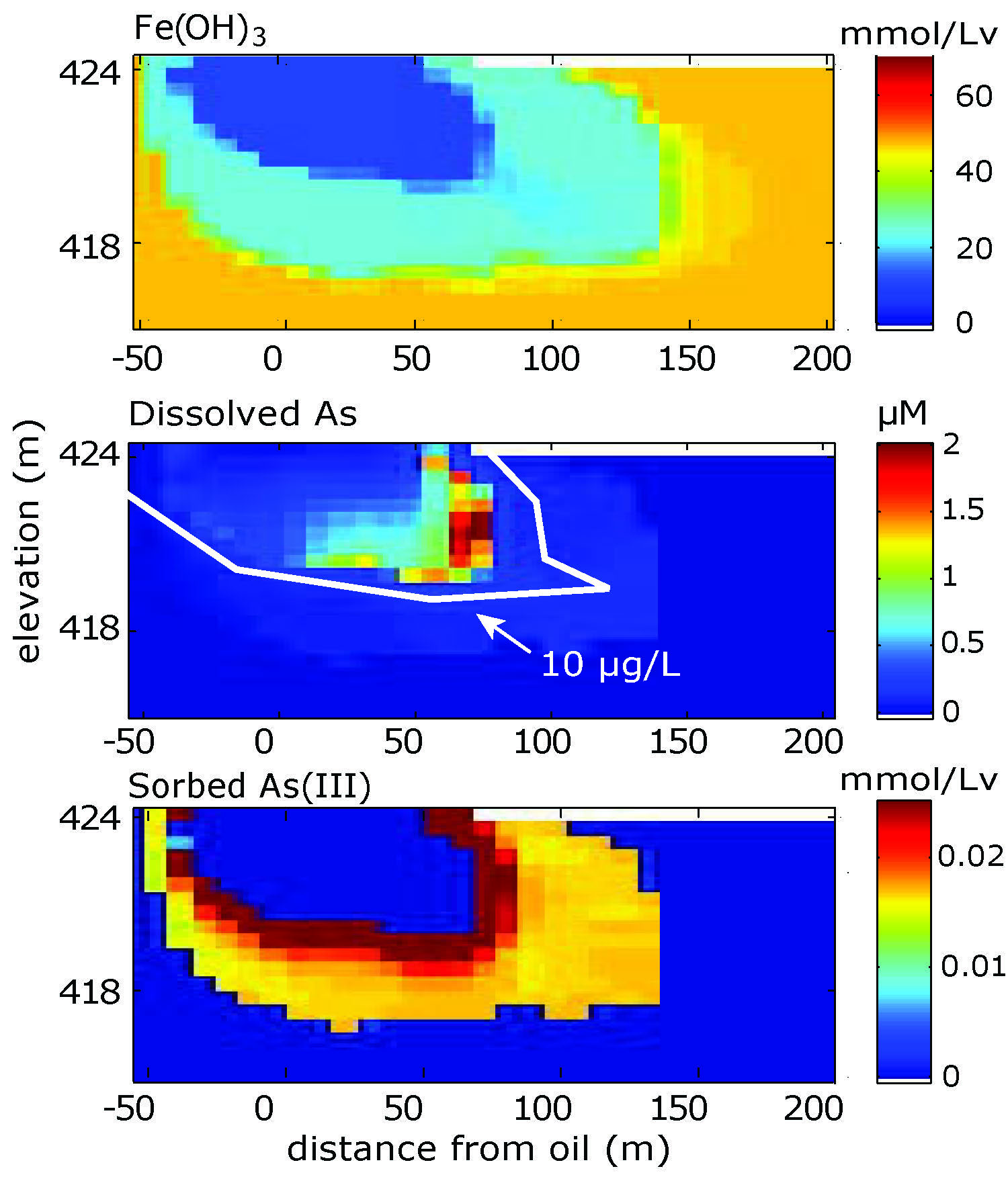
Study Site
2. Methods
2.1. Model Domain and Hydrogeologic Parameters
2.2. Geochemical Formulation
2.3. Initial Conditions
2.4. Calibration Approach
2.5. Model Sensitivity
3. Results and Discussion
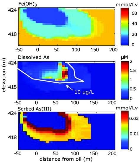
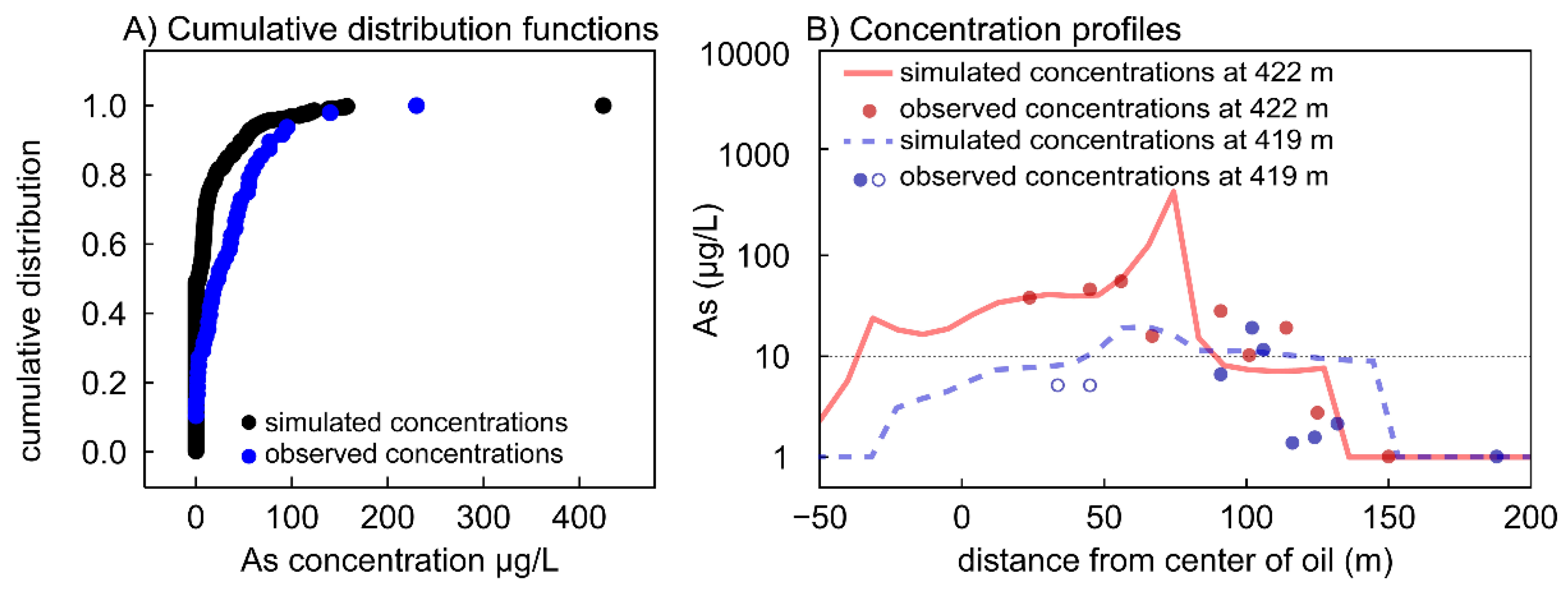
3.1. Calibrated Model Results
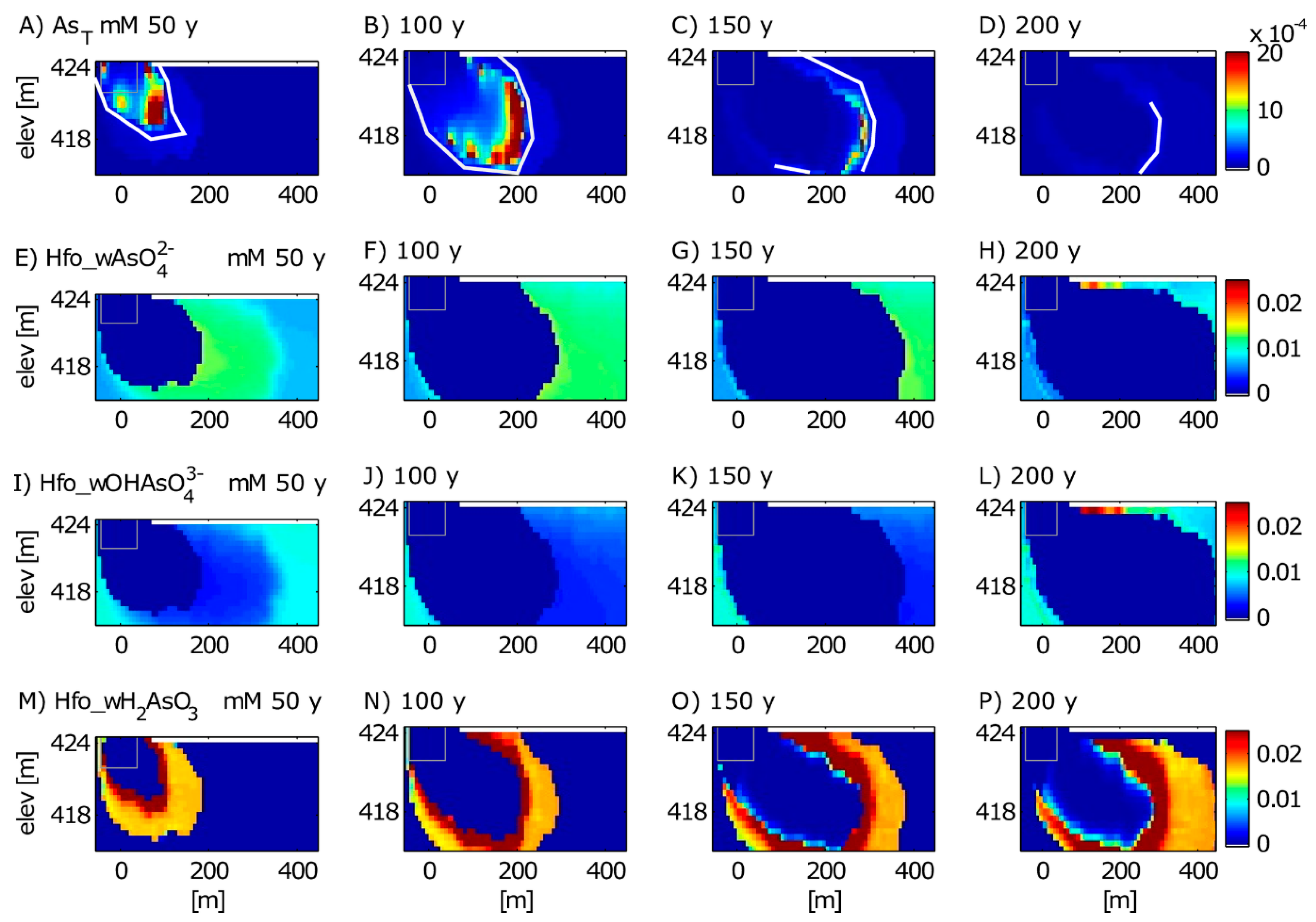
3.1.1. Aqueous Species
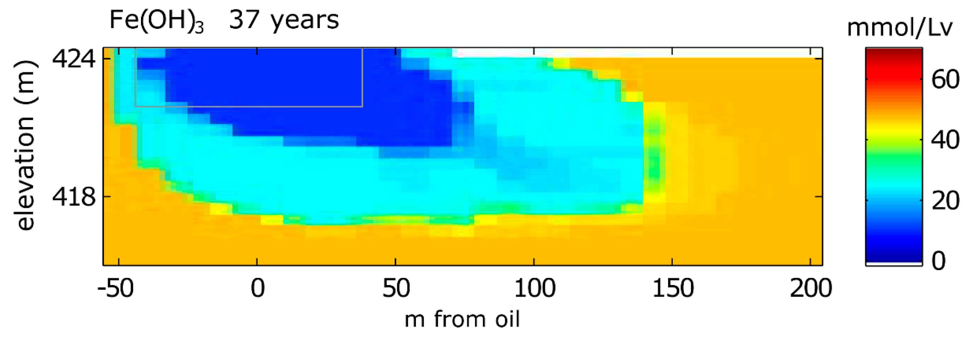
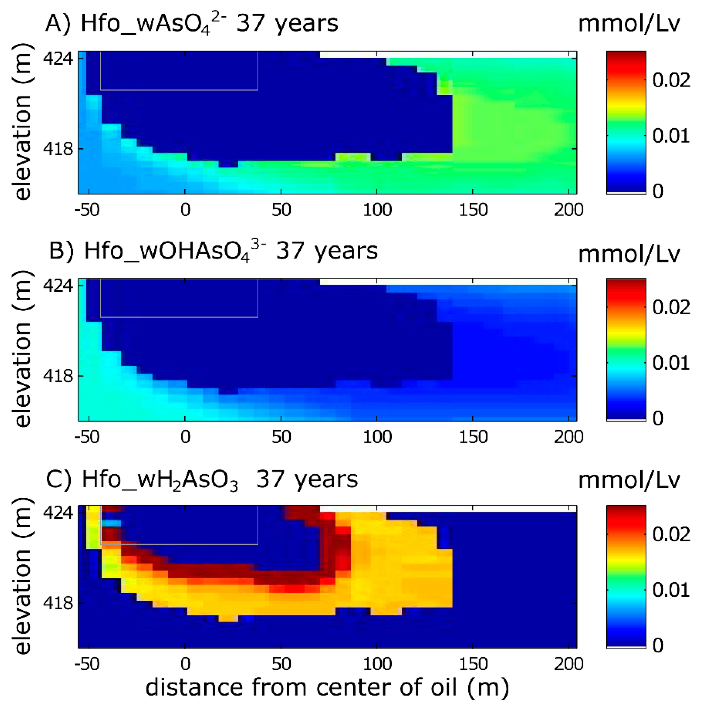
3.1.2. Solid Phase Species
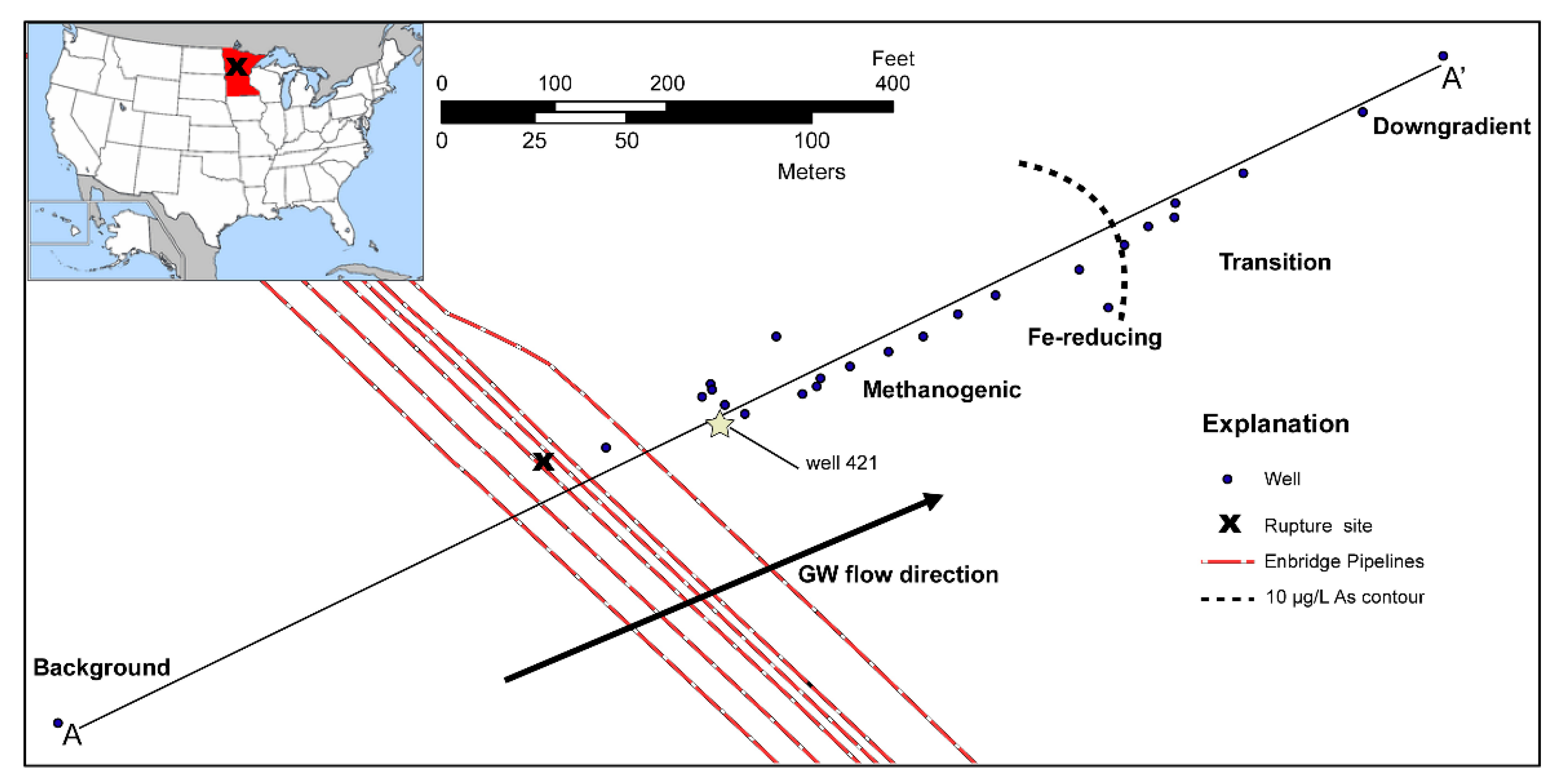
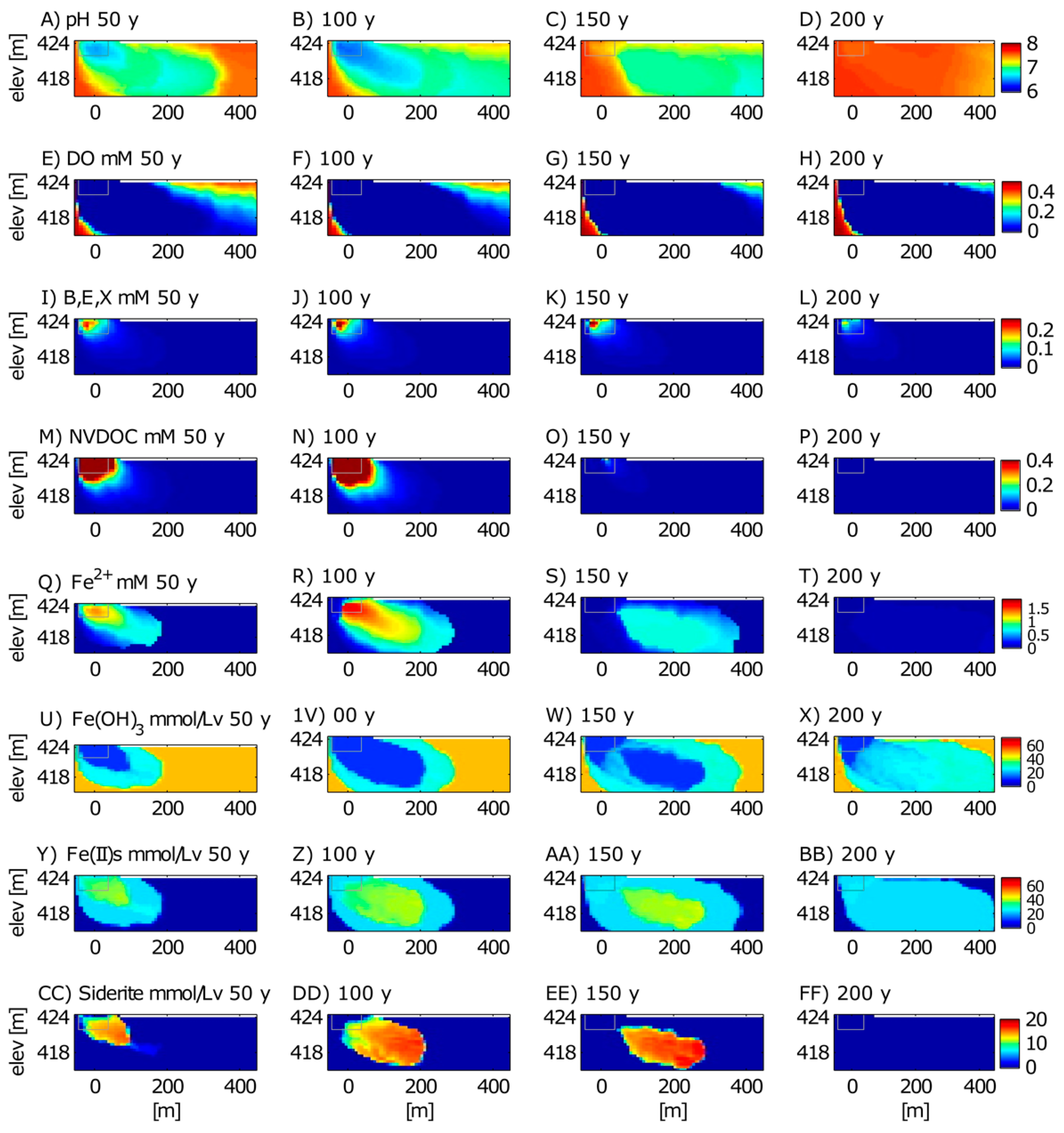
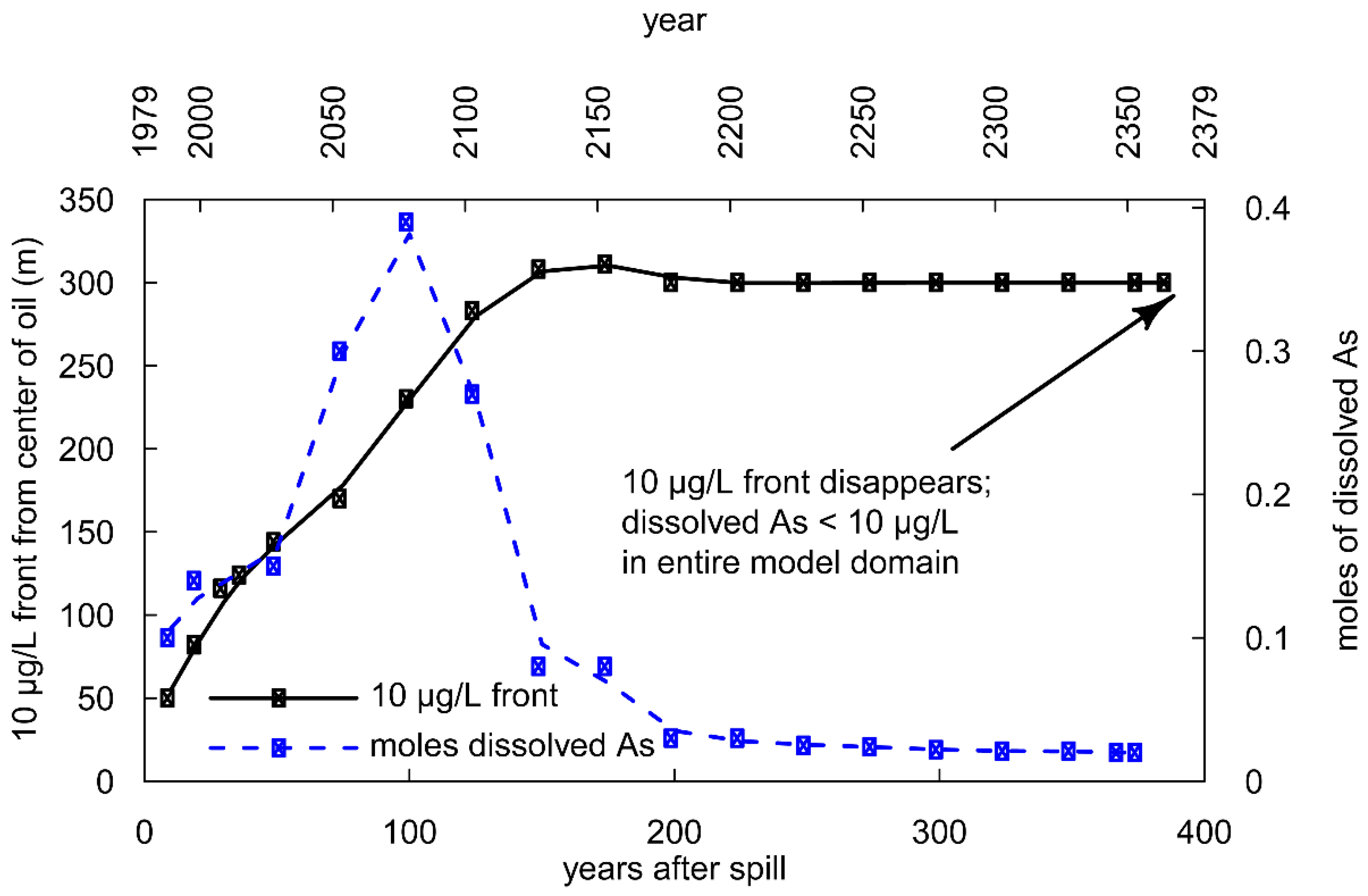
3.2. Long-Term Cycling of As in the Petroleum Hydrocarbon Plume
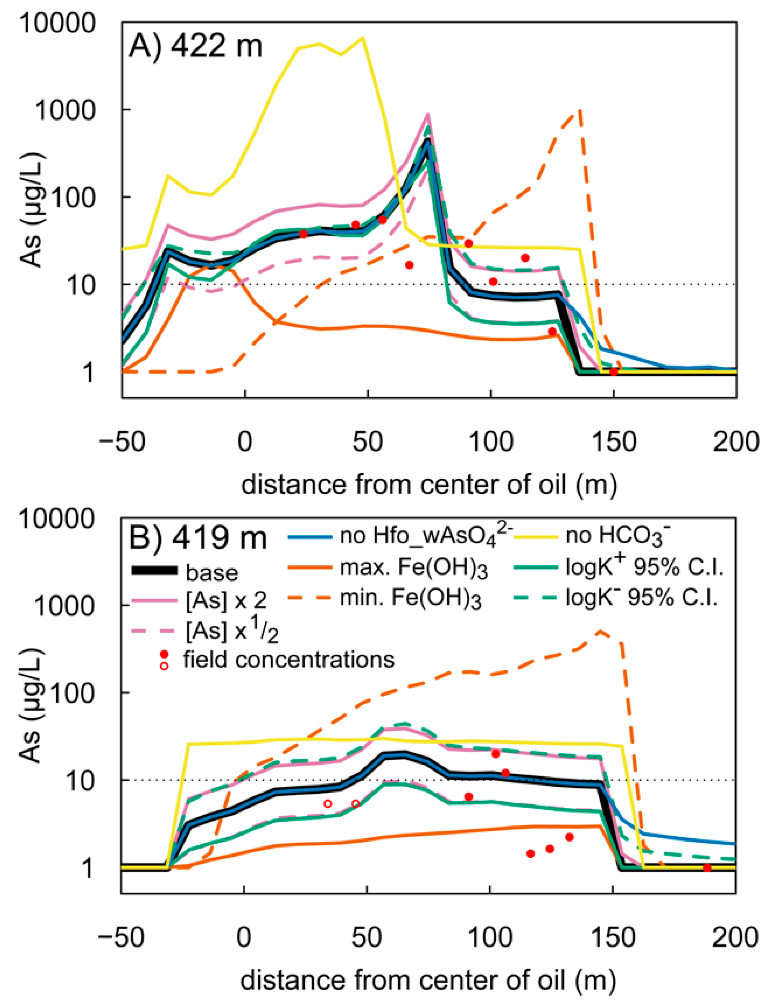
3.3. Model Sensitivity
3.4. Model Limitations
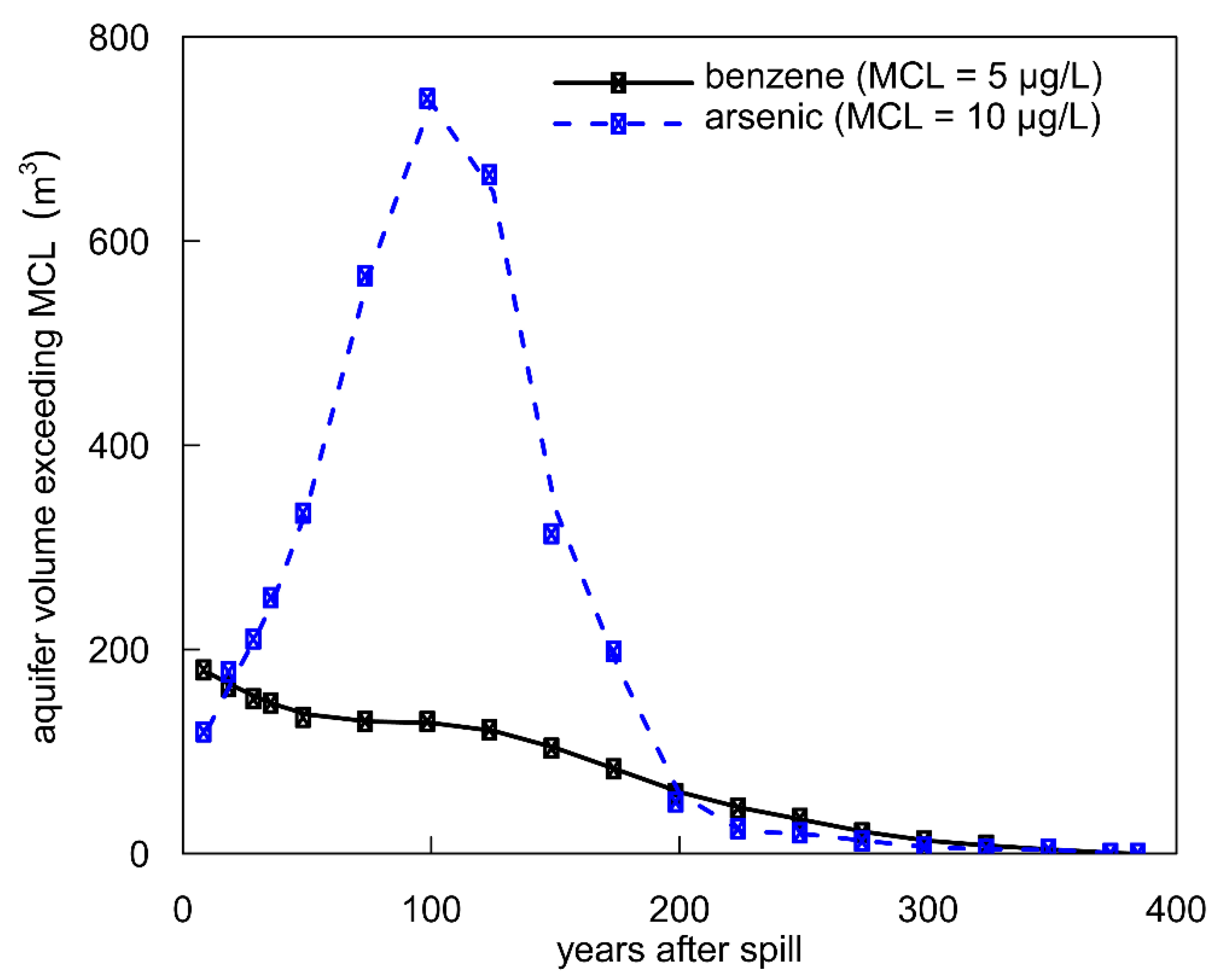
3.5. Human Health Consequences
4. Conclusions and Opportunities for Future Research
Supplementary Materials
Author Contributions
Funding
Institutional Review Board Statement
Informed Consent Statement
Data Availability Statement
Acknowledgments
Conflicts of Interest
References
- National Research Council. Critical Aspects of EPA’s IRIS Assessment of Inorganic Arsenic: Interm Report; National Academy Press: Washington, DC, USA, 2014.
- United States Environmental Protection Agency. Drinking Water Standard for Arsenic; EPA 815-F-00-016; United States Environmental Protection Agency: Washington, DC, USA, 2001.
- Nordstrom, D.K. Worldwide occurrences of arsenic in ground water. Science 2002, 296, 2143LP–2145LP. [Google Scholar] [CrossRef] [PubMed]
- Smedley, P.L.; Kinniburgh, D.G. A review of the source, behaviour and distribution of arsenic in natural waters. Appl. Geochem. 2002, 17, 517–568. [Google Scholar] [CrossRef]
- Welch, A.H.; Westjohn, D.B.; Helsel, D.R.; Wanty, R.B. Arsenic in ground water of the united states: Occurrence and geochemistry. Groundwater 2000, 38, 589–604. [Google Scholar] [CrossRef]
- Sø, H.U.; Postma, D.; Vi, M.L.; Pham, T.K.T.; Kazmierczak, J.; Dao, V.N.; Pi, K.; Koch, C.B.; Pham, H.V.; Jakobsen, R. Arsenic in holocene aquifers of the Red River Floodplain, Vietnam: Effects of sediment-water interactions, sediment burial age and groundwater residence time. Geochim. Cosmochim. Acta 2018, 225, 192–209. [Google Scholar] [CrossRef]
- Harvey, C.F.; Swartz, C.H.; Badruzzaman, A.B.M.; Keon-Blute, N.; Yu, W.; Ali, M.A.; Jay, J.; Beckie, R.; Niedan, V.; Brabander, D.; et al. Arsenic mobility and groundwater extraction in Bangladesh. Science 2002, 298, 1602LP–1606LP. [Google Scholar] [CrossRef]
- Neumann, R.B.; Pracht, L.E.; Polizzotto, M.L.; Badruzzaman, A.B.M.; Ali, M.A. Biodegradable organic carbon in sediments of an arsenic-contaminated aquifer in Bangladesh. Environ. Sci. Technol. Lett. 2014, 1, 221–225. [Google Scholar] [CrossRef]
- Neumann, R.B.; Ashfaque, K.N.; Badruzzaman, A.B.M.; Ashraf Ali, M.; Shoemaker, J.K.; Harvey, C.F. Anthropogenic influences on groundwater arsenic concentrations in Bangladesh. Nat. Geosci. 2010, 3, 46–52. [Google Scholar] [CrossRef]
- Polizzotto, M.L.; Kocar, B.D.; Benner, S.G.; Sampson, M.; Fendorf, S. Near-surface wetland sediments as a source of arsenic release to ground water in Asia. Nature 2008, 454, 505–508. [Google Scholar] [CrossRef]
- Whaley-Martin, K.J.; Mailloux, B.J.; van Geen, A.; Bostick, B.C.; Ahmed, K.M.; Choudhury, I.; Slater, G.F. Human and livestock waste as a reduced carbon source contributing to the release of arsenic to shallow Bangladesh groundwater. Sci. Total Environ. 2017, 595, 63–71. [Google Scholar] [CrossRef]
- Kocar, B.D.; Fendorf, S. Thermodynamic constraints on reductive reactions influencing the biogeochemistry of arsenic in soils and sediments. Environ. Sci. Technol. 2009, 43, 4871–4877. [Google Scholar] [CrossRef]
- Postma, D.; Larsen, F.; Thai, N.T.; Trang, P.T.K.; Jakobsen, R.; Nhan, P.Q.; Long, T.V.; Viet, P.H.; Murray, A.S. Groundwater arsenic concentrations in Vietnam controlled by sediment age. Nat. Geosci. 2012, 5, 656–661. [Google Scholar] [CrossRef]
- Stuckey, J.W.; Sparks, D.L.; Fendorf, S. Delineating the Convergence of Biogeochemical Factors Responsible for Arsenic Release to Groundwater in South and Southeast Asia; Sparks, D.L., Ed.; Academic Press: Cambridge, MA, USA, 2016; Volume 140, pp. 43–74. [Google Scholar] [CrossRef]
- Stuckey, J.W.; Schaefer, M.V.; Benner, S.G.; Fendorf, S. Reactivity and speciation of mineral-associated arsenic in seasonal and permanent wetlands of the Mekong Delta. Geochim. Cosmochim. Acta 2015, 171, 143–155. [Google Scholar] [CrossRef]
- Radloff, K.A.; Zheng, Y.; Michael, H.A.; Stute, M.; Bostick, B.C.; Mihajlov, I.; Bounds, M.; Huq, M.R.; Choudhury, I.; Rahman, M.W.; et al. Arsenic migration to deep groundwater in Bangladesh influenced by adsorption and water demand. Nat. Geosci. 2011, 4, 793–798. [Google Scholar] [CrossRef]
- van Geen, A.; Zheng, Y.; Goodbred, S.; Horneman, A.; Aziz, Z.; Cheng, Z.; Stute, M.; Mailloux, B.; Weinman, B.; Hoque, M.A.; et al. Flushing history as a hydrogeological control on the regional distribution of arsenic in shallow groundwater of the Bengal Basin. Environ. Sci. Technol. 2008, 42, 2283–2288. [Google Scholar] [CrossRef][Green Version]
- Postma, D.; Mai, N.T.H.; Lan, V.M.; Trang, P.T.K.; Sø, H.U.; Nhan, P.Q.; Larsen, F.; Viet, P.H.; Jakobsen, R. Fate of Arsenic during red river water tnfiltration into aquifers beneath Hanoi, Vietnam. Environ. Sci. Technol. 2017, 51, 838–845. [Google Scholar] [CrossRef] [PubMed]
- Stute, M.; Zheng, Y.; Schlosser, P.; Horneman, A.; Dhar, R.K.; Datta, S.; Hoque, M.A.; Seddique, A.A.; Shamsudduha, M.; Ahmed, K.M.; et al. Hydrological control of as concentrations in Bangladesh groundwater. Water Resour. Res. 2007, 43. [Google Scholar] [CrossRef]
- Charlet, L.; Chakraborty, S.; Appelo, C.A.J.; Roman-Ross, G.; Nath, B.; Ansari, A.A.; Lanson, M.; Chatterjee, D.; Mallik, S.B. Chemodynamics of an arsenic hotspot in a West Bengal aquifer: A field and reactive transport modeling study. Appl. Geochem. 2007, 22, 1273–1292. [Google Scholar] [CrossRef]
- Jung, H.B.; Bostick, B.C.; Zheng, Y. Field, experimental, and modeling study of arsenic partitioning across a redox transition in a Bangladesh aquifer. Environ. Sci. Technol. 2012, 46, 1388–1395. [Google Scholar] [CrossRef]
- Postma, D.; Larsen, F.; Minh Hue, N.T.; Duc, M.T.; Viet, P.H.; Nhan, P.Q.; Jessen, S. Arsenic in groundwater of the red river floodplain, Vietnam: Controlling geochemical processes and reactive transport modeling. Geochim. Cosmochim. Acta 2007, 71, 5054–5071. [Google Scholar] [CrossRef]
- Rotiroti, M.; Jakobsen, R.; Fumagalli, L.; Bonomi, T. Arsenic release and attenuation in a multilayer aquifer in the po plain (Northern Italy): Reactive transport modeling. Appl. Geochem. 2015, 63, 599–609. [Google Scholar] [CrossRef]
- Wallis, I.; Prommer, H.; Berg, M.; Siade, A.J.; Sun, J.; Kipfer, R. The river–groundwater interface as a hotspot for arsenic release. Nat. Geosci. 2020, 13, 288–295. [Google Scholar] [CrossRef]
- Johannesson, K.H.; Yang, N.; Trahan, A.S.; Telfeyan, K.; Jade Mohajerin, T.; Adebayo, S.B.; Akintomide, O.A.; Chevis, D.A.; Datta, S.; White, C.D. Biogeochemical and reactive transport modeling of arsenic in groundwaters from the Mississippi River Delta plain: An analog for the As-affected aquifers of South and Southeast Asia. Geochim. Cosmochim. Acta 2019, 264, 245–272. [Google Scholar] [CrossRef]
- Jung, H.B.; Charette, M.A.; Zheng, Y. Field, Laboratory, and modeling study of reactive transport of groundwater arsenic in a coastal aquifer. Environ. Sci. Technol. 2009, 43, 5333–5338. [Google Scholar] [CrossRef]
- Rawson, J.; Siade, A.; Sun, J.; Neidhardt, H.; Berg, M.; Prommer, H. Quantifying reactive transport processes governing arsenic mobility after injection of reactive organic carbon into a Bengal Delta aquifer. Environ. Sci. Technol. 2017, 51, 8471–8480. [Google Scholar] [CrossRef] [PubMed]
- Ng, G.-H.C.; Bekins, B.A.; Cozzarelli, I.M.; Baedecker, M.J.; Bennett, P.C.; Amos, R.T.; Herkelrath, W.N. Reactive transport modeling of geochemical controls on secondary water quality impacts at a crude oil spill site near Bemidji, MN. Water Resour. Res. 2015, 51, 4156–4183. [Google Scholar] [CrossRef]
- Cozzarelli, I.M.; Schreiber, M.E.; Erickson, M.L.; Ziegler, B.A. Arsenic cycling in hydrocarbon plumes: Secondary effects of natural attenuation. Groundwater 2016, 54, 35–45. [Google Scholar] [CrossRef]
- Ziegler, B.A.; Schreiber, M.E.; Cozzarelli, I.M. The role of alluvial aquifer sediments in attenuating a dissolved arsenic plume. J. Contam. Hydrol. 2017, 204, 90–101. [Google Scholar] [CrossRef] [PubMed]
- Ziegler, B.A.; Schreiber, M.E.; Cozzarelli, I.M.; Crystal Ng, G.-H. A mass balance approach to investigate arsenic cycling in a petroleum plume. Environ. Pollut. 2017, 231, 1351–1361. [Google Scholar] [CrossRef] [PubMed]
- Bekins, B.A.; Cozzarelli, I.M.; Curtis, G.P. A simple method for calculating growth rates of petroleum hydrocarbon plumes. Groundwater 2005, 43, 817–826. [Google Scholar] [CrossRef] [PubMed]
- Cozzarelli, I.M.; Bekins, B.A.; Eganhouse, R.P.; Warren, E.; Essaid, H.I. In situ measurements of volatile aromatic hydrocarbon biodegradation rates in groundwater. J. Contam. Hydrol. 2010, 111, 48–64. [Google Scholar] [CrossRef]
- Cozzarelli, I.M.; Baedecker, M.J.; Eganhouse, R.P.; Goerlitz, D.F. The geochemical evolution of low-molecular-weight organic acids derived from the degradation of petroleum contaminants in groundwater. Geochim. Cosmochim. Acta 1994, 58, 863–877. [Google Scholar] [CrossRef]
- Eganhouse, R.P.; Baedecker, M.J.; Cozzarelli, I.M.; Aiken, G.R.; Thorn, K.A.; Dorsey, T.F. Crude oil in a shallow sand and gravel aquifer—II. Organic geochemistry. Appl. Geochem. 1993, 8, 551–567. [Google Scholar] [CrossRef]
- Essaid, H.I.; Bekins, B.A.; Herkelrath, W.N.; Delin, G.N. Crude oil at the Bemidji site: 25 years of monitoring, modeling, and understanding. Groundwater 2011, 49, 706–726. [Google Scholar] [CrossRef] [PubMed]
- Lovley, D.R.; Baedecker, M.J.; Lonergan, D.J.; Cozzarelli, I.M.; Phillips, E.J.P.; Siegel, D.I. Oxidation of aromatic contaminants coupled to microbial iron reduction. Nature 1989, 339, 297–300. [Google Scholar] [CrossRef]
- Tuccillo, M.E.; Cozzarelli, I.M.; Herman, J.S. Iron reduction in the sediments of a hydrocarbon-contaminated aquifer. Appl. Geochem. 1999, 14, 655–667. [Google Scholar] [CrossRef]
- Baedecker, M.J. Authigenic Mineral Formation in Aquifer Rich in Organic Material. In Water-Rock Interaction-7; Karkaka, Y.K., Maest, A.S., Eds.; International Association of Geochemistry and Cosmochemistry: Rotterdam, The Netherlands, 1992; pp. 257–263. [Google Scholar]
- Zachara, J.M.; Kukkadapu, R.K.; Gassman, P.L.; Dohnalkova, A.; Fredrickson, J.K.; Anderson, T. Biogeochemical transformation of fe minerals in a petroleum-contaminated aquifer. Geochim. Cosmochim. Acta 2004, 68, 1791–1805. [Google Scholar] [CrossRef]
- Essaid, H.I.; Cozzarelli, I.M.; Eganhouse, R.P.; Herkelrath, W.N.; Bekins, B.A.; Delin, G.N. Inverse modeling of BTEX dissolution and biodegradation at the Bemidji, MN crude-oil spill site. J. Contam. Hydrol. 2003, 67, 269–299. [Google Scholar] [CrossRef]
- Dillard, L.A.; Essaid, H.I.; Herkelrath, W.N. Multiphase flow modeling of a crude-oil spill site with a bimodal permeability distribution. Water Resour. Res. 1997, 33, 1617–1632. [Google Scholar] [CrossRef]
- Strobel, M.L.; Delin, G.N.; Munson, C.J. Spatial Variation in Saturated Hydraulic Conductivity of Sediments at a Crude-Oil Spill Site near Bemidji, Minnesota; Water-Resources Investigations Report 98-4503; U.S. Geological Survey: Mounds View, MN, USA, 1998.
- Bennett, P.C.; Siegel, D.E.; Baedecker, M.J.; Hult, M.F. Crude oil in a shallow sand and gravel aquifer—I. Hydrogeology and inorganic geochemistry. Appl. Geochem. 1993, 8, 529–549. [Google Scholar] [CrossRef]
- Pipeline and Hazardous Materials Safety Administration. Hazardous Liquid Pipeline Accident Reports for 2010–Present; Updated 30 April 2020; U.S. Department of Transportation: Washington, DC, USA, 2020.
- Pfannkuch, H.O. Interim Report and Recommendations on Monitoring Program for Site M.P. 926.5; Unpublished Consultant Report; Lakehead Pipe Line Company, Inc.: Calgary, AB, Canada, 1979. [Google Scholar]
- Baedecker, M.J.; Cozzarelli, I.M.; Eganhouse, R.P.; Siegel, D.I.; Bennett, P.C. Crude oil in a shallow sand and gravel aquifer—III. Biogeochemical reactions and mass balance modeling in anoxic groundwater. Appl. Geochem. 1993, 8, 569–586. [Google Scholar] [CrossRef]
- Cozzarelli, I.M.; Bekins, B.A.; Baedecker, M.J.; Aiken, G.R.; Eganhouse, R.P.; Tuccillo, M.E. Progression of natural attenuation processes at a crude-oil spill site: I. Geochemical evolution of the plume. J. Contam. Hydrol. 2001, 53, 369–385. [Google Scholar] [CrossRef]
- Amos, R.T.; Bekins, B.A.; Cozzarelli, I.M.; Voytek, M.A.; Kirshtein, J.D.; Jones, E.J.P.; Blowes, D.W. Evidence for iron-mediated anaerobic methane oxidation in a crude oil-contaminated aquifer. Geobiology 2012, 10, 506–517. [Google Scholar] [CrossRef]
- McNab, W.W., Jr.; Narasimhan, T.N. Modeling reactive transport of organic compounds in groundwater using a partial redox disequilibrium approach. Water Resour. Res. 1994, 30, 2619–2635. [Google Scholar] [CrossRef]
- Essaid, H.I.; Bekins, B.A.; Godsy, E.M.; Warren, E.; Baedecker, M.J.; Cozzarelli, I.M. Simulation of aerobic and anaerobic biodegradation processes at a crude oil spill site. Water Resour. Res. 1995, 31, 3309–3327. [Google Scholar] [CrossRef]
- Curtis, G.P. Comparison of approaches for simulating reactive solute transport involving organic degradation reactions by multiple terminal electron acceptors. Comput. Geosci. 2003, 29, 319–329. [Google Scholar] [CrossRef]
- Amos, R.T.; Mayer, U.K. Investigating the role of gas bubble formation and entrapment in contaminated aquifers: Reactive transport modelling. J. Contam. Hydrol. 2006, 87, 123–154. [Google Scholar] [CrossRef]
- Prommer, H.; Barry, D.A.; Zheng, C. MODFLOW/MT3DMS-based reactive multicomponent transport modeling. Groundwater 2003, 41, 247–257. [Google Scholar] [CrossRef] [PubMed]
- Harbaugh, A.W. MODFLOW-2005: The U.S. Geological Survey Modular Ground-Water Model-the Ground-Water Flow Process; U.S. Geological Survey: Reston, VA, USA, 2005. [CrossRef]
- Zheng, C.; Wang, P.P. MT3DMS: A Modular Three-Dimensional Multispecies Model for Simulation of Advection, Dispersion and Chemical Reactions of Contaminants in Groundwater Systems: Documentation and User’s Guide; Development Center Contract Report SERDP-99-1; U.S. Army Engineer Research: Vicksburg, MI, USA, 1999. [Google Scholar]
- Parkhurst, D.L.; Appelo, C.A.J. User’s Guide to PHREEQC (Version 2)-A Computer Program for Speciation, Batch-Reaction, One-Dimensional Transport, and Inverse Geochemical Calculations; Water-Resources Investigations Report 99-4259; U.S. Geological Survey: Denver, CO, USA, 1999.
- Jakobsen, R.; Postma, D. Redox zoning, rates of sulfate reduction and interactions with fe-reduction and methanogenesis in a shallow sandy aquifer, Rømø, Denmark. Geochim. Cosmochim. Acta 1999, 63, 137–151. [Google Scholar] [CrossRef]
- Dzombak, D.A.; Morel, F.M. Surface Complexation Modeling: Hydrous Ferric Oxide; John Wiley & Sons: Hoboken, NJ, USA, 1990. [Google Scholar]
- Smith, R.M.; Martell, A.E. Critical Stability Constants, Inorganic Complexes; Plenum Press: New York, NY, USA, 1976; Volume 4. [Google Scholar]
- Dixit, S.; Hering, J.G. Comparison of arsenic(V) and arsenic(III) sorption onto iron oxide minerals: Implications for arsenic mobility. Environ. Sci. Technol. 2003, 37, 4182–4189. [Google Scholar] [CrossRef]
- Appelo, C.A.J.; Van Der Weiden, M.J.J.; Tournassat, C.; Charlet, L. Surface complexation of ferrous iron and carbonate on ferrihydrite and the mobilization of arsenic. Environ. Sci. Technol. 2002, 36, 3096–3103. [Google Scholar] [CrossRef]
- Ziegler, B.A.; Schreiber, M.E.; Cozzarelli, I.M.; Ng, G.-H.C. Arsenic and Iron Data (2010–2015) for Petroleum Plume Mass Balance; U.S. Geological Survey: Bemidji, MN, USA, 2017. [CrossRef]
- Ng, G.-H.C.; Bekins, B.A.; Cozzarelli, I.M.; Baedecker, M.J.; Bennett, P.C.; Amos, R.T. A mass balance approach to investigating geochemical controls on secondary water quality impacts at a crude oil spill site near Bemidji, MN. J. Contam. Hydrol. 2014, 164, 1–15. [Google Scholar] [CrossRef]
- Heron, G.; Crouzet, C.; Bourg, A.C.M.; Christensen, T.H. Speciation of Fe(II) and Fe(III) in contaminated aquifer sediments using chemical extraction techniques. Environ. Sci. Technol. 1994, 28, 1698–1705. [Google Scholar] [CrossRef] [PubMed]
- Barcelona, M.J.; Varljen, M.D.; Puls, R.W.; Kaminski, D. Ground water purging and sampling methods: History vs. hysteria. Groundw. Monit. Remediat. 2005, 25, 52–62. [Google Scholar] [CrossRef]
- Erickson, M.L.; Malenda, H.F.; Berquist, E.C.; Ayotte, J.D. Arsenic concentrations after drinking water well installation: Time-varying effects on arsenic mobilization. Sci. Total Environ. 2019, 678, 681–691. [Google Scholar] [CrossRef] [PubMed]
- Erickson, M.L.; Barnes, R.J. Arsenic concentration variability in public water system wells in Minnesota, USA. Appl. Geochem. 2006, 21, 305–317. [Google Scholar] [CrossRef]
- Schreiber, M.E.; Simo, J.A.; Freiberg, P.G. Stratigraphic and geochemical controls on naturally occurring arsenic in groundwater, Eastern Wisconsin, USA. Hydrogeol. J. 2000, 8, 161–176. [Google Scholar] [CrossRef]
- Zheng, C.; Bennett, G.D. Applied Contaminant Transport Modeling; Wiley-Interscience: New York, NY, USA, 2002. [Google Scholar]
- Anawar, H.M.; Akai, J.; Sakugawa, H. Mobilization of arsenic from subsurface sediments by effect of bicarbonate ions in groundwater. Chemosphere 2004, 54, 753–762. [Google Scholar] [CrossRef] [PubMed]
- Bekins, B.A.; Cozzarelli, I.M.; Godsy, E.M.; Warren, E.; Essaid, H.I.; Tuccillo, M.E. Progression of natural attenuation processes at a crude oil spill site: II. Controls on spatial distribution of microbial populations. J. Contam. Hydrol. 2001, 53, 387–406. [Google Scholar] [CrossRef]
- Eganhouse, R.P.; Dorsey, T.F.; Phinney, C.S.; Westcott, A.M. Processes affecting the fate of monoaromatic hydrocarbons in an aquifer contaminated by crude oil. Environ. Sci. Technol. 1996, 30, 3304–3312. [Google Scholar] [CrossRef]
- Podgorski, J.; Berg, M. Global threat of arsenic in groundwater. Science 2020, 368, 845LP–850LP. [Google Scholar] [CrossRef] [PubMed]
- Lee, J.-U.; Lee, S.-W.; Kim, K.-W.; Yoon, C.-H. The effects of different carbon sources on microbial mediation of arsenic in arsenic-contaminated sediment. Environ. Geochem. Health 2005, 27, 159–168. [Google Scholar] [CrossRef] [PubMed]
- McLean, J.E.; Dupont, R.R.; Sorensen, D.L. Iron and arsenic release from aquifer solids in response to biostimulation. J. Environ. Qual. 2006, 35, 1193–1203. [Google Scholar] [CrossRef] [PubMed]
- Smith, S.; Dupont, R.R.; McLean, J.E. Arsenic release and attenuation processes in a groundwater aquifer during anaerobic remediation of TCE with biostimulation. Groundw. Monit. Remediat. 2019, 39, 61–70. [Google Scholar] [CrossRef]
- Tillotson, J.M.; Borden, R.C. Statistical analysis of secondary water quality impacts from enhanced reductive bioremediation. Groundw. Monit. Remediat. 2015, 35, 67–77. [Google Scholar] [CrossRef]


| logK | logK −95% C.I. b | logK +95% C.I. c | Ref. | ||
|---|---|---|---|---|---|
| Acid dissociation reactions a | |||||
| 1 | H3AsO4 = H2AsO4− + H+ | 2.24 | [60] | ||
| 2 | H2AsO4− = HAsO42− + H+ | 6.96 | [60] | ||
| 3 | HAsO42− = AsO43− + H+ | 11.5 | [60] | ||
| 4 | H3AsO3 = H2AsO3− + H+ | 9.29 | |||
| Surface (de)protonation reactions | |||||
| 5 | Hfo_wOH + H+ = Hfo_wOH2+ | 7.29 | |||
| 6 | Hfo_wOH = Hfo_wO− + H+ | −8.93 | [59] | ||
| Arsenate (As(V)) reaction | |||||
| 7 | Hfo_wOH + AsO43− + 3H+ = Hfo_wH2AsO4 + H2O | 29.31 | 28.29 | 30.34 | [59] |
| 8 | Hfo_wOH + AsO43− + 2H+ = Hfo_wHAsO4− + H2O | 23.51 | 23.33 | 23.7 | [59] |
| 9 | Hfo_wOH + AsO43− + H+ = Hfo_wAsO42− + H2O | 18.1 | [61] | ||
| 10 | Hfo_wOH + AsO43− = Hfo_wOHAsO43− | 10.58 | 10.01 | 11.15 | [59] |
| Arsenite (As(III)) reactions | |||||
| 11 | Hfo_wOH + H3AsO3 = Hfo_wH2AsO3 + H2O | 5.41 | 5.11 | 5.71 | [59] |
| Bicarbonate reaction | |||||
| 12 | Hfo_wOH + CO32− + 2H+ = Hfo_wHCO3 + H2O | 20.37 | 19.39 | 21.35 | [62] |
| Hfo_wOH + CO32− + H+ = Hfo_wCO3− + H2O | 12.78 | 12.58 | 12.98 | [62] | |
| Aqueous Phase | Input Background | Equilibrated |
|---|---|---|
| As(III) (mol/L; mg/L) | 3 × 10⁻¹⁰; 2.25 × 10⁻⁵ | 0.00; 0.00 |
| As(V) (mol/L; mg/L) | 0.00; 0.00 | 3 × 10⁻¹⁰; 2.25 × 10⁻⁵ |
| Total carbonates (mol/L; mg/L) | 3.69 × 10⁻³; 225 | 3.65 × 10⁻³; 222 |
| CH4 (mol/L; mg/L) | 6.23 × 10⁻⁷; 9.99 × 10⁻³ | 0.00; 0.00 |
| Ca2+ (mol/L; mg/L) | 1.28 × 10⁻³; 51.7 | 1.25 × 10⁻³; 50.1 |
| Cl− (mol/L; mg/L) | 3.10 × 10⁻⁴; 11.0 | 3.10 × 10⁻⁴; 11.0 |
| Fe2+ (mol/L; mg/L) | 0.00; 0.00 | 5.05 × 10⁻²⁴; 2.8 × 10⁻¹⁹ |
| Mg2+ (mol/L; mg/L) | 5.95 × 10⁻⁴; 14.5 | 5.95 × 10⁻⁴; 14.5 |
| Na+ (mol/L; mg/L) | 7.70 × 10⁻⁵; 1.77 | 7.70 × 10⁻⁵; 1.77 |
| O2 (mol/L; mg/L) | 4.94 × 10⁻⁴; 15.8 | 4.92 × 10⁻⁴; 15.7 |
| Mn2+ (mol/L; mg/L) | 0.00; 0.00 | 0.00; 0.00 |
| N2 (mol/L; mg/L) | 4.49 × 10⁻⁴; 12.6 | 4.49 × 10⁻⁴; 12.6 |
| pH (standard units) | 7.72 | 7.63 |
| pe (standard units) | 14.47 | 14.30 |
| Sensitivity of: | logK | Initial Fe(OH)3 (mol/Lv) | Initial Sorbed As (mmol/Lv) | |||
|---|---|---|---|---|---|---|
| Base: Mean | Base: 0.0370 | Base: 1.62 × 10⁻² | ||||
| Decrease | Increase | Decrease | Increase | Decrease | Increase | |
| log(K) −95% C.I. | log(K) +95% C.I. | Lowest Measured Background: 0.0228 | Greatest Measured Background: 0.0657 | Half: 3.7 × 10⁻² | Double: 3.24 × 10⁻² | |
| Location of 10 μg/L As front | −0.46 | −0.09 | −0.43 | −1.05 | 0.08 | 0.79 |
| Total dissolved As mass | −0.06 | −0.12 | −14.36 | −0.12 | 1.01 | 1.00 |
| Maximum dissolved As | 0.08 | −0.09 | −11.75 | 2.27 | 1.02 | 1.05 |
Publisher’s Note: MDPI stays neutral with regard to jurisdictional claims in published maps and institutional affiliations. |
© 2021 by the authors. Licensee MDPI, Basel, Switzerland. This article is an open access article distributed under the terms and conditions of the Creative Commons Attribution (CC BY) license (https://creativecommons.org/licenses/by/4.0/).
Share and Cite
Ziegler, B.A.; Ng, G.-H.C.; Cozzarelli, I.M.; Dunshee, A.J.; Schreiber, M.E. Arsenic in Petroleum-Contaminated Groundwater near Bemidji, Minnesota Is Predicted to Persist for Centuries. Water 2021, 13, 1485. https://doi.org/10.3390/w13111485
Ziegler BA, Ng G-HC, Cozzarelli IM, Dunshee AJ, Schreiber ME. Arsenic in Petroleum-Contaminated Groundwater near Bemidji, Minnesota Is Predicted to Persist for Centuries. Water. 2021; 13(11):1485. https://doi.org/10.3390/w13111485
Chicago/Turabian StyleZiegler, Brady A., G.-H. Crystal Ng, Isabelle M. Cozzarelli, Aubrey J. Dunshee, and Madeline E. Schreiber. 2021. "Arsenic in Petroleum-Contaminated Groundwater near Bemidji, Minnesota Is Predicted to Persist for Centuries" Water 13, no. 11: 1485. https://doi.org/10.3390/w13111485
APA StyleZiegler, B. A., Ng, G.-H. C., Cozzarelli, I. M., Dunshee, A. J., & Schreiber, M. E. (2021). Arsenic in Petroleum-Contaminated Groundwater near Bemidji, Minnesota Is Predicted to Persist for Centuries. Water, 13(11), 1485. https://doi.org/10.3390/w13111485