Predicting BOD under Various Hydrological Conditions in the Dongjin River Basin Using Physics-Based and Data-Driven Models

Abstract

The water quality of the Dongjin River deteriorates during the irrigation period because the supply of river maintenance water to the main river is cut off by the mass intake of agricultural weirs located in the midstream regions. A physics-based model and a data-driven model were used to predict the water quality in the Dongjin River under various hydrological conditions. The Hydrological Simulation Program–Fortran (HSPF), which is a physics-based model, was constructed to simulate the biological oxygen demand (BOD) in the Dongjin River Basin. A Gamma Test was used to derive the optimal combinations of the observed variables, including external water inflow, water intake, rainfall, and flow rate, for irrigation and non-irrigation periods. A data-driven adaptive neuro-fuzzy inference system (ANFIS) model was then built using these results. The ANFIS model built in this study was capable of predicting the BOD from the observed hydrological data in the irrigation and non-irrigation periods, without running the physics-based model. The predicted results have high confidence levels when compared with the observed data. Thus, the proposed method can be used for the reliable and rapid prediction of water quality using only monitoring data as input.

1. Introduction

The Saemangeum project in Korea, pursued for over three decades, involves building the longest sea dike in the world for the reclamation of land and lakes with the goals of expanding land area, developing water resources, and providing extra land for farming. However, with increasing concerns regarding water pollution due to accelerated development, alleviating water pollution and achieving the target water quality have emerged as key factors. Currently, a large quantity of river water is used for agriculture through large irrigation systems in the Mangyeong and Dongjin River basins, which drain into the Saemangeum Lake. This has significantly hampered the flow of rivers and increased their susceptibility to drying up, leading to difficulties in water quality management [1]. The Ministry of Environment (MOE) conducted a quantitative assessment of the effects of the Master Plans for Water Quality Improvement using water quality modeling techniques. They found that the increase in the external water inflow had the largest effect on water quality improvement. Hence, the ministry proposed measures to secure the flow rate, including an increase in the discharges from the Yongdam and Seomjin River Dams to the upstream regions of the Mangyeong and Dongjin Rivers [2]. In particular, the water quality of the Dongjin River deteriorates during the irrigation period due to the mass intake of river maintenance water at the Nakyang Weir, a diversion weir located in the midstream region of the Dongjin River.

Therefore, it is necessary to analyze and predict water quality according to the complex hydrological conditions for an effective water quality management in the Dongjin River Basin. To achieve this, a physics-based model or data-driven model can be applied [3]. A physics-based model enables the prediction of water quality by treating the watershed as a closed system and formulating, applying, and analyzing all physical, chemical, and biological mechanisms present in the system. However, as there are numerous models available, an appropriate model must be selected based on the characteristics and choice of water quality parameters of the target watershed, while also considering the purpose of the analysis and available computing power. Furthermore, as various input data are required, it is difficult to estimate the optimal parameters, and the subjective interpretations of model developers may introduce data biases. Conversely, data-driven models have a better structure for analyzing complex nonlinear relationships between input and output data (i.e., water quality) [4], reduce data uncertainty by relearning in response to environmental changes, and produce relatively reliable data. However, describing these structures and relationships are complex. Examples of data-driven models include artificial neural networks (ANNs), genetic algorithms, and fuzzy models.

Faruk [4] developed a hybrid model using an autoregressive integrated moving average model and an ANN to predict water quality from time-series data. Khadr et al. [5] constructed an adaptive neuro-fuzzy inference system (ANFIS) model to predict total phosphorus (TP) and total nitrogen (TN). Sarkar and Pandey [6] used the feed forward error back propagation algorithm, which is an ANN technique, to predict dissolved oxygen (DO). Najah et al. [7] used an ANN to predict dissolved solids, electrical conductivity, and turbidity. These studies constructed data-driven models based on actual observed data obtained on a monthly timescale or longer. In Korea, water quality has been estimated using observed data from the water quality monitoring networks of the MOE. Among these networks, official water quality measurements supported by the largest quantity of data comprise total maximum daily load (TMDL) monitoring network data (measured every 8 days); however, the quantity of data is insufficient to build a data-driven model based only on the observed data [8,9]. In addition, according to Park et al. [10], the TMDL monitoring network data are not fully representative of the overall flow rate because only approximately 40 observations are made per year, and if water quality measurements are concentrated during specific flow conditions (i.e., dry conditions and low flows), the water quality reflecting these conditions will be overrepresented.

In this study, we propose an efficient technique for predicting the water quality of the Dongjin River Basin, which combines the advantages of physics-based and data-driven models (Figure 1). First, a physics-based model, Hydrological Simulation Program—Fortran (HSPF), was employed to reproduce the daily water quality according to various hydrological conditions and pollutant discharge loads in the Dongjin River Basin. Additionally, the Adaptive Neuro-Fuzzy Inference System (ANFIS) model, which is a data-driven model, was constructed to maximally reflect the variability of the water quality according to various hydrological conditions, enabling rapid and accurate water quality predictions.

2. Materials and Methods

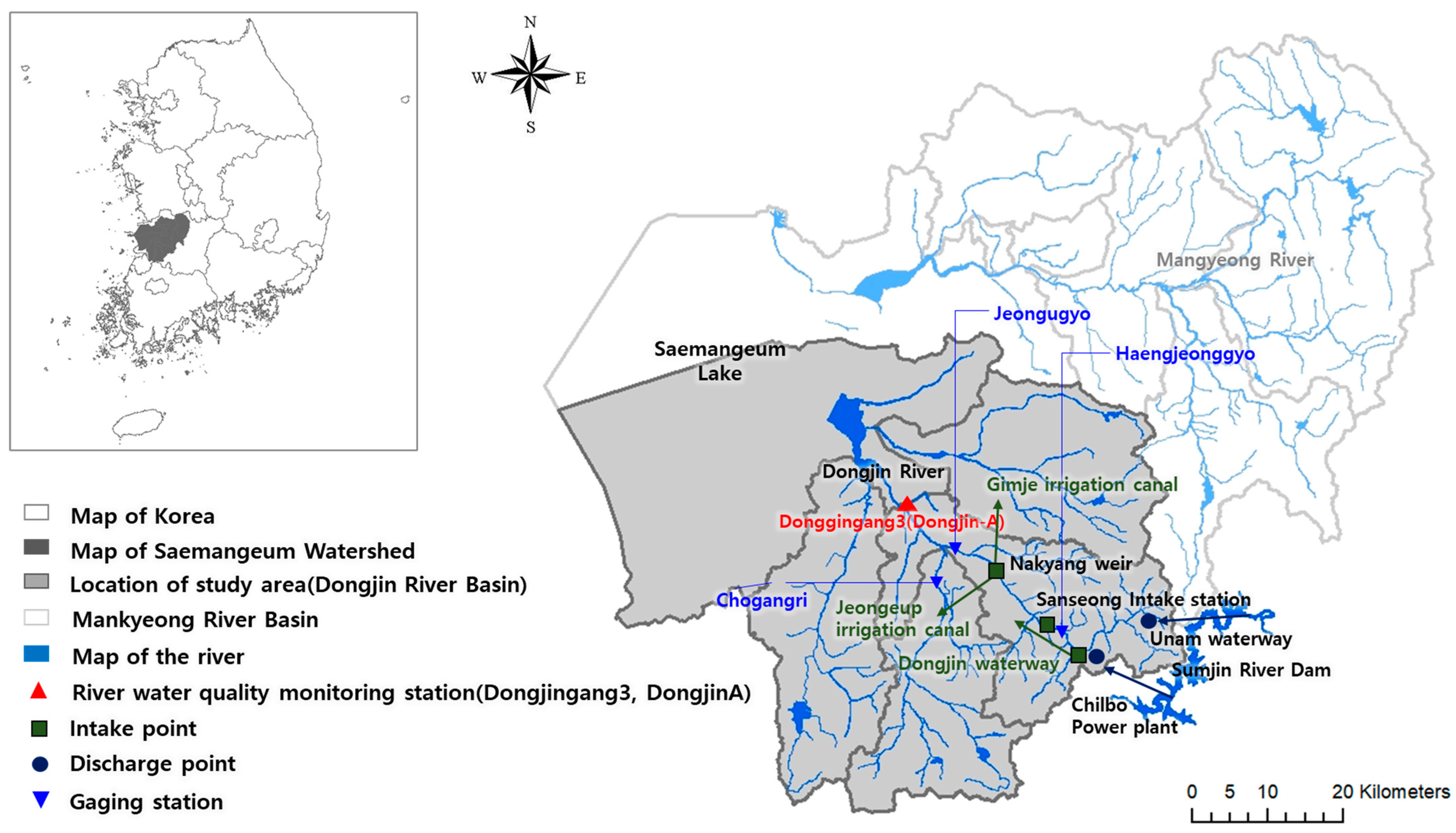
2.1. Study Area and Scope

The Saemangeum Watershed is divided into the Mangyeong River, Dongjin River, and is part of the west coast, with a total area of 3319 km². The target water quality of Saemangeum Lake is grade 4 (COD ≤ 8.0 mg/L, TP ≤ 0.100 mg/L, and Chl-a ≤ 35.0 mg/m³) for the midstream and upstream regions, which comprises agricultural land according to the land use plan, and grade 3 (COD ≤ 5.0 mg/L, TP ≤ 0.050 mg/L, and Chl-a ≤ 20.0 mg/m³) for the downstream region, planned for tourism and urban development. To achieve the target water quality for Saemangeum Lake, the pollutant load from the Mangyeong and Dongjin Rivers must be minimized first. The area selected for this study was the Dongjin River Basin, with an area of 1397.0 km², of which 629.7 km² is agricultural land, accounting for approximately 45.1% of the total area. This is approximately twice the average agricultural area in Korea (23%). Thus, the water quality of this region is expected to be significantly affected by agricultural inputs and utilization systems [11].

The flow of water through the Dongjin River Basin is illustrated in Figure 2. Water from the Seomjin River Dam flows through the Unam waterway and the Chilbo power plant in the upstream part of the Dongjin River. The water from the Chilbo power plant is then diverted into the Dongjin waterway, located immediately downstream of the plant. Some of the water from the Dongjin River is collected at the Sanseong intake station for domestic use. Then, at the Nakyang Weir, located midstream of the Dongjin River, most of the water is supplied for irrigation to the Gimje and Jeongeup irrigation canals. For 11 years (2008–2018), the Dongjin River Basin has received approximately 83% (413.7 million m³/year) of the total discharge (496.7 million m³/year) of the Seomjin River Dam. 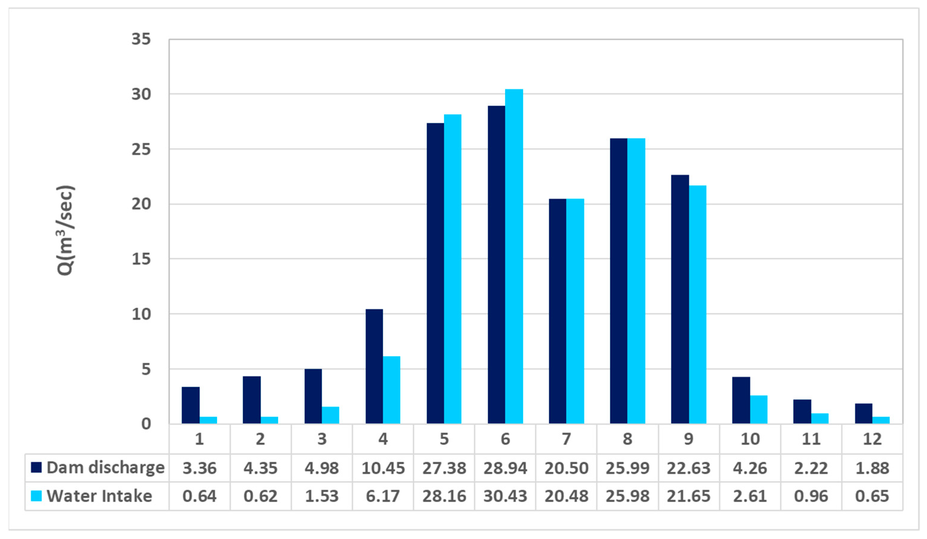As shown in Figure 3, the monthly discharge begins to increase from April with the advent of the irrigation period; it is largest in June at 28.9 m³/s, and smallest in December at 1.9 m³/s. Approximately 90% of this discharge is used for agricultural and domestic purposes. Because there are no regulatory standards for water intake, most of the dam discharge is consumed during the irrigation period, except when flooding occurs. Hence, the actual flow rate of water to the main Dongjin River downstream of the Nakyang Weir is very limited.

To reflect the hydrological characteristics of the Dongjin River Basin in our water quality predictions, irrigation and non-irrigation periods were differentiated. The irrigation water supply period in the water-use license for the Seomjin River Dam is from 20 April to 30 September annually. Based on this, the period from April to September was set as the irrigation period, and October to March was set as the non-irrigation period.

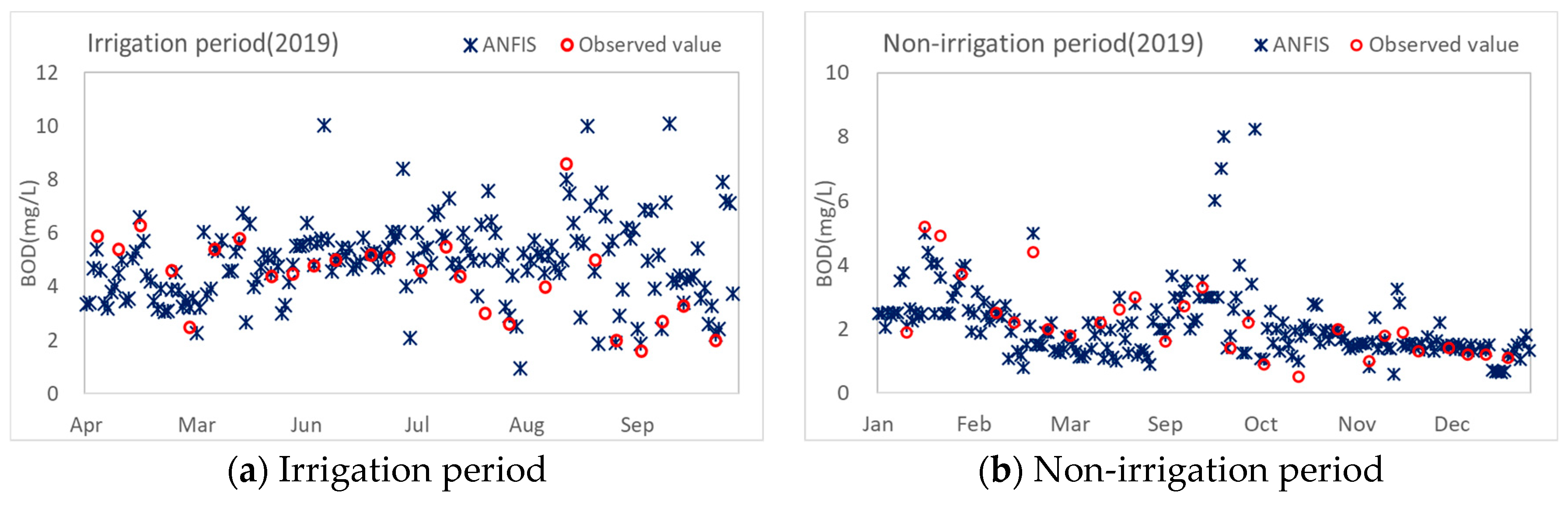
The Dongjin River 3 (Dongjin A), situated at the end of the Dongjin River, was selected as the site for water quality predictions, as the target water quality is monitored here according to Korea’s Water Environmental Management Plans. Dongjin River 3 is a river management monitoring station situated upstream of the Saemangeum Lake, wherein the target water quality, in terms of biological oxygen demand (BOD), must be achieved within a specific planned year.

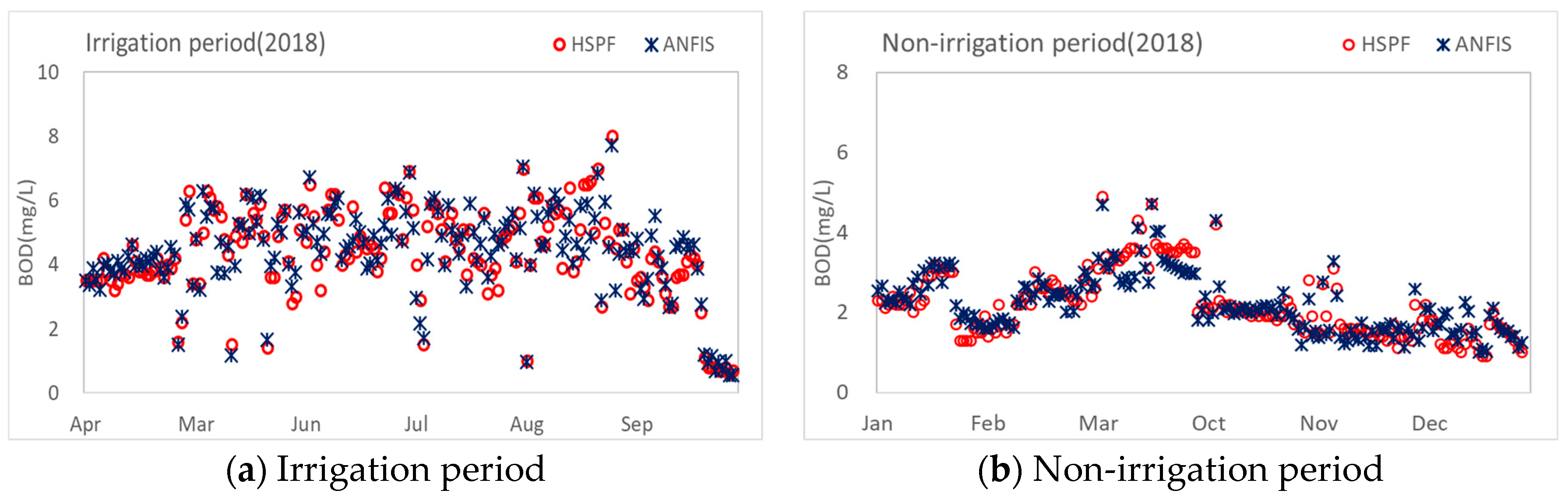
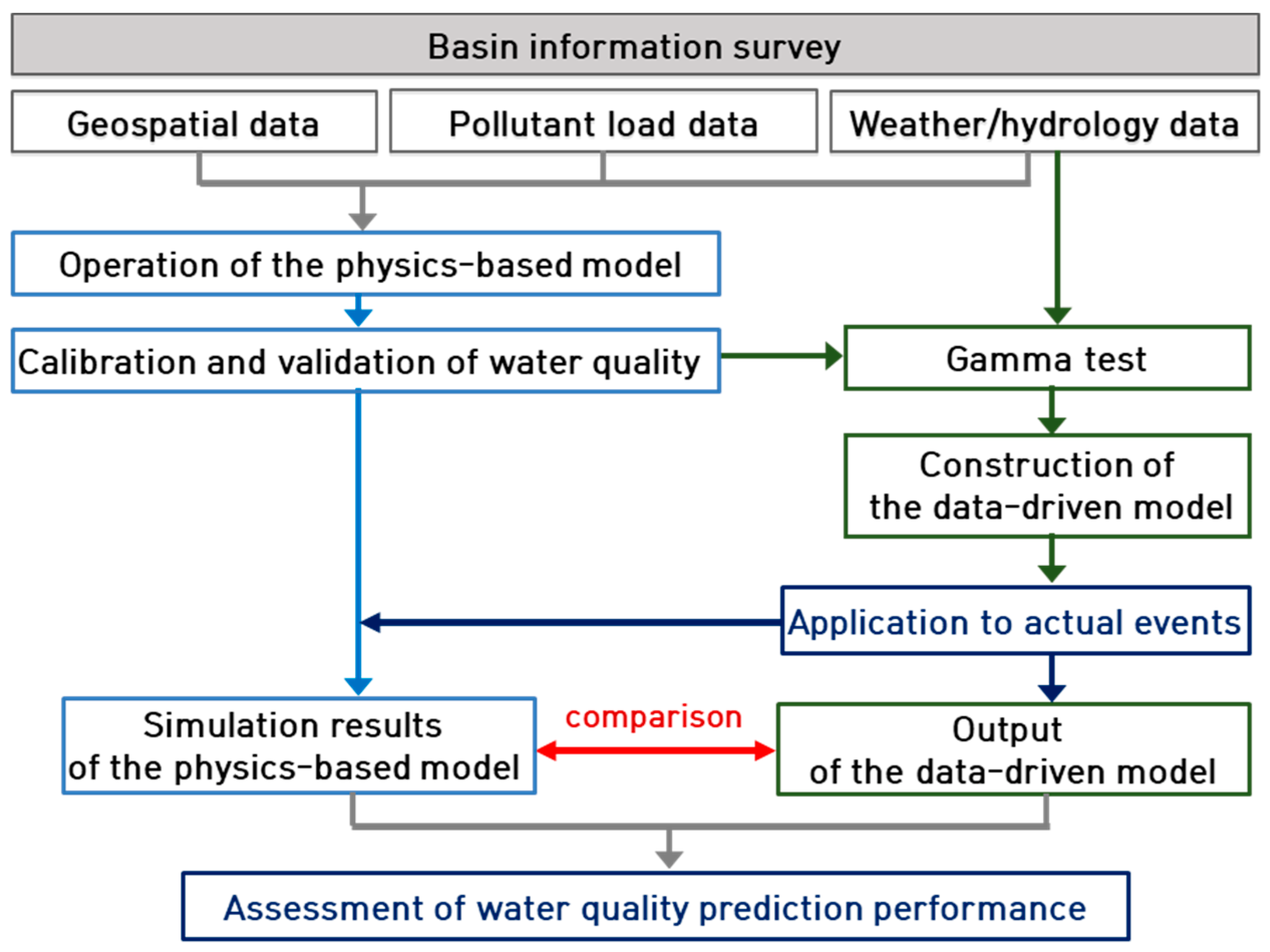
The duration considered for the physics-based model was approximately 11 years (from 2007–2018). Excluding the stabilization period, the calibration and validation periods were set based on recent data. The learning period for constructing the data-driven model was divided into irrigation and non-irrigation periods. Approximately 10 years of data from 2008 to 2017 were used, and the applicability of the data-driven model developed in this study was assessed using the HSPF simulation results for 2018.

2.2. Physics-Based Model

The HSPF model is appropriate for simulating the runoff and water quality of a watershed in both urban and rural or mountainous areas to analyze water quality variations depending on the daily and seasonal pollutant discharge characteristics [12]. To use the HSPF model, basic information was input using the better assessment science integrating point and non-point sources (BASINS), which is an integrated management system that manages significant amounts of data based on Geographic Information System (GIS) and supports various models. First, a river network was generated by calculating the flow direction and flow accumulation from a digital elevation model, and it was segmented by specifying the exit point of the watershed as the outlet. Land cover was classified into seven categories: urban or built-up land, wetland, agricultural land, forest land, pastureland, barren land, and water. Then, the land use information for each segmented sub-watershed was extracted using the land use and soil definition utility of the model.

With regard to meteorological parameters, seven types of observed values for each hour, including rainfall, temperature, dew point, cloud cover, solar radiation, wind speed, and evapotranspiration were input into the model. Among the disaggregate functions included in WDMUtil, the evapotranspiration function was used to generate evapotranspiration data.

The pollutant load data calculated from the pollutant source data for the 2008–2018 period were input to obtain point-source pollutant load data. The daily water discharge and the quality data of discharged water (BOD, SS, TN, and TP) were collected and input for the sewage treatment facilities which recorded daily average discharges of 500 m³ or higher (Sintaein, Jeongeup, Buan, and Gimje).

Daily hydrological data including dam discharge (Unam waterway and Chilbo power plant) and water intake (Dongjin waterway, Nakyang Weir, and Sanseong intake station) for agricultural and domestic uses were surveyed and used as the daily inputs.

2.3. Calibration and Validation of the HSPF Model

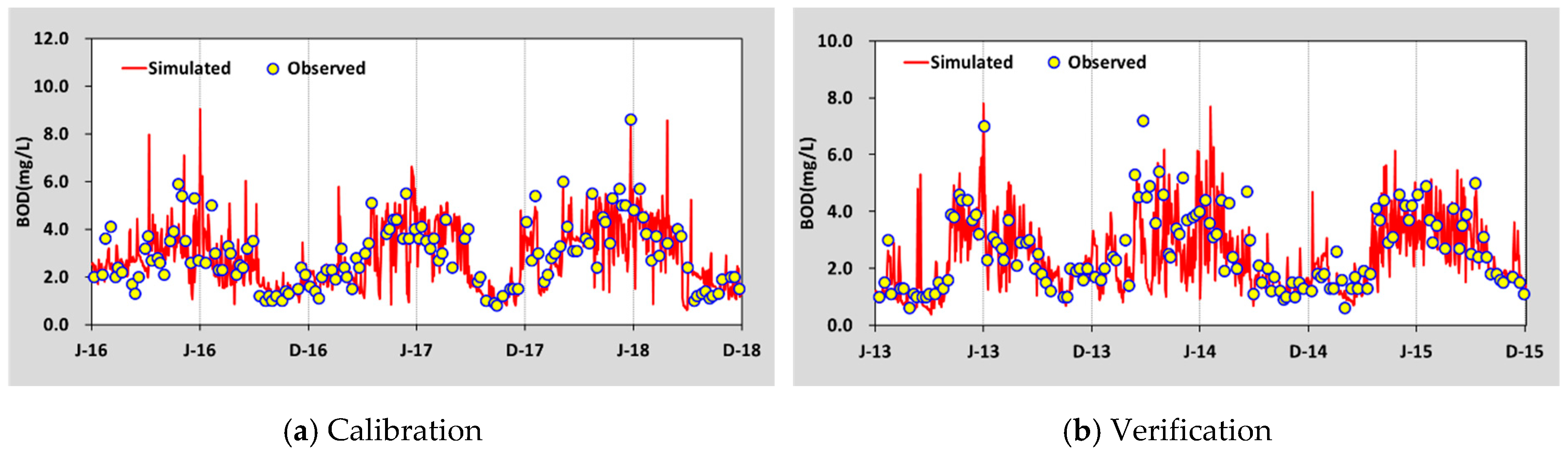
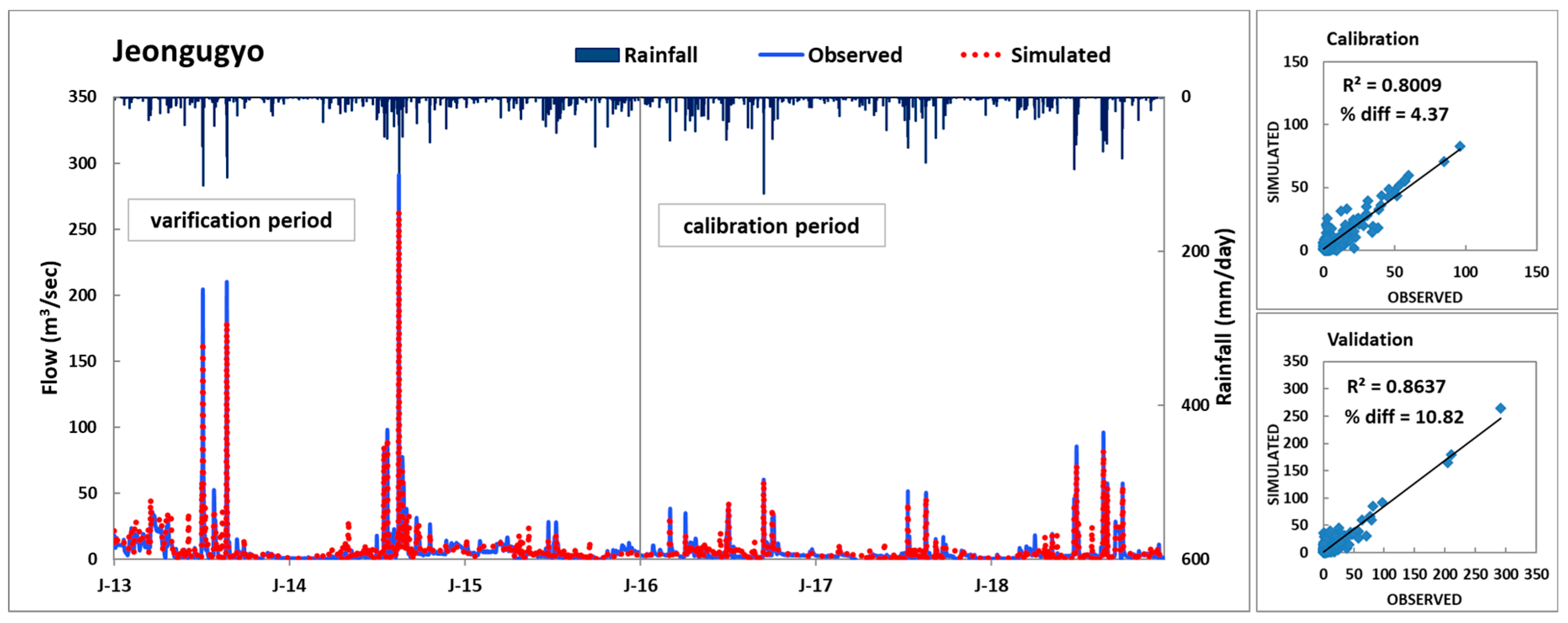
The flow rates measured at the three gauging stations, Haengjeonggyo, Chogangri, and Jeongugyo, were used for the calibration and validation of the HSPF model. The Total Maximum Daily Loads (TMDL) monitoring network data measured at Dongjin A, approximately 40 times per year at the end of each unit of watershed, were used for the water quality assessments. The calibration and validation periods were 2016–2018 and 2013–2015, respectively. The calibration and validation were conducted every three years, and their periods were defined based on the water quality data that could be collected.

To evaluate the accuracy of the calibration and validation results for the flow rate, the coefficient of determination (R²) was calculated, and the criteria in

Table 1. General calibration/validation target or tolerance for HSPF application.

Criteria	Very Good	Good	Fair	Poor
R2	>0.8	0.8–0.7	0.7–0.6	<0.6

suggested by Donigian [13] were used. In the case of water quality, to evaluate the appropriateness of the simulation results for the measured values, the percentage difference confidence interval listed in the BASINS/HSPF Training Lecture (

Table 2. Percentage difference for model performance.

Constituent	Very Good	Good	Fair
Hydrology/Flow	<10	10–15	15–25
Water Quality	<15	15–25	25–35

) as well as the average (0.89), range (0.71–0.61), and root mean square error (RMSE) of the actual measured values and the simulation values were calculated.

$$RMSE=\sqrt[]{\frac{{\sum }_{i=1}^N{\left(P_i-O_i\right)}^2}{N},}$$

(1)

where P_i denotes the predicted values, O_i denotes the observed values, and N is the total number of observations.

The parameters of flow rate applied in this study were adjusted to the following variables: lower zone nominal soil moisture storage (LZSN), infiltration capacity of the soil (INFILT), basic groundwater recession rate (AGWRC), fraction of groundwater inflow which will enter deep groundwater (DEEPER), interflow inflow (INTEW), and interflow recession (IRC;

Table 3. HSPF parameter values for hydrological simulation.

Parameter	Definition	Typical Range	Final Calibrated Value	Jaswinder et al. (2005) [14]	Ribarova et al. (2008) [15]
LZSN	Lower zone nominal soil moisture storage (in)	3.00–8.00	4.90–12.00	5.00	15.00
INFILT	Infiltration capacity of the soil (in/h)	0.010–0.25	0.06–0.10	0.20	0.05–0.16
AGWRC	Basic groundwater recession rate (1/day)	0.92–0.99	0.98	0.98	0.99
DEEPER	Fraction of groundwater inflow which will enter deep groundwater	0.00–2.00	0.05	0.05	0.15
INTEW	Interflow inflow parameter	1.00–10.00	1.00–2.00	1.20–1.80	1.25
IRC	Interflow recession parameter (1/day)	0.30–0.85	0.30–0.80	0.60–0.80	0.3.

). In the case of water quality calibration, the water temperature and DO were first calibrated, followed by the BOD. Table 3 and

Table 4. HSPF parameter values for the water quality simulations.

Parameter	Definition	Unit	Typical Range	Final Calibrated Value	Jang (2010) [16]	Jeon (2011) [17]
KBOD20	BOD decay rate at 20 °C	1/h	0.001–0.140	0.002–0.006	0.011–0.015	0.004–0.067
KODSET	Rate of BOD settling	ft/h	>0	0.001–0.027	0.018–0.033	0.011–0.027
REAK	Reaeration coefficient	1/h	-	0.20	0.48	0.05–0.20
CVBO	Conversion from milligrams biomass to milligrams oxygen	mg/mg	1.00–5.00	1.00–2.70	-	1.63
CVBPC	Conversion from biomass expressed as phosphorus to carbon	moles/mol	50–200	106–180	-	106
CVBPN	Conversion from biomass expressed as phosphorus to nitrogen	moles/mol	-	16	-	-

show the parameters applied in this study and those applied in the previous studies.

2.4. Gamma Test

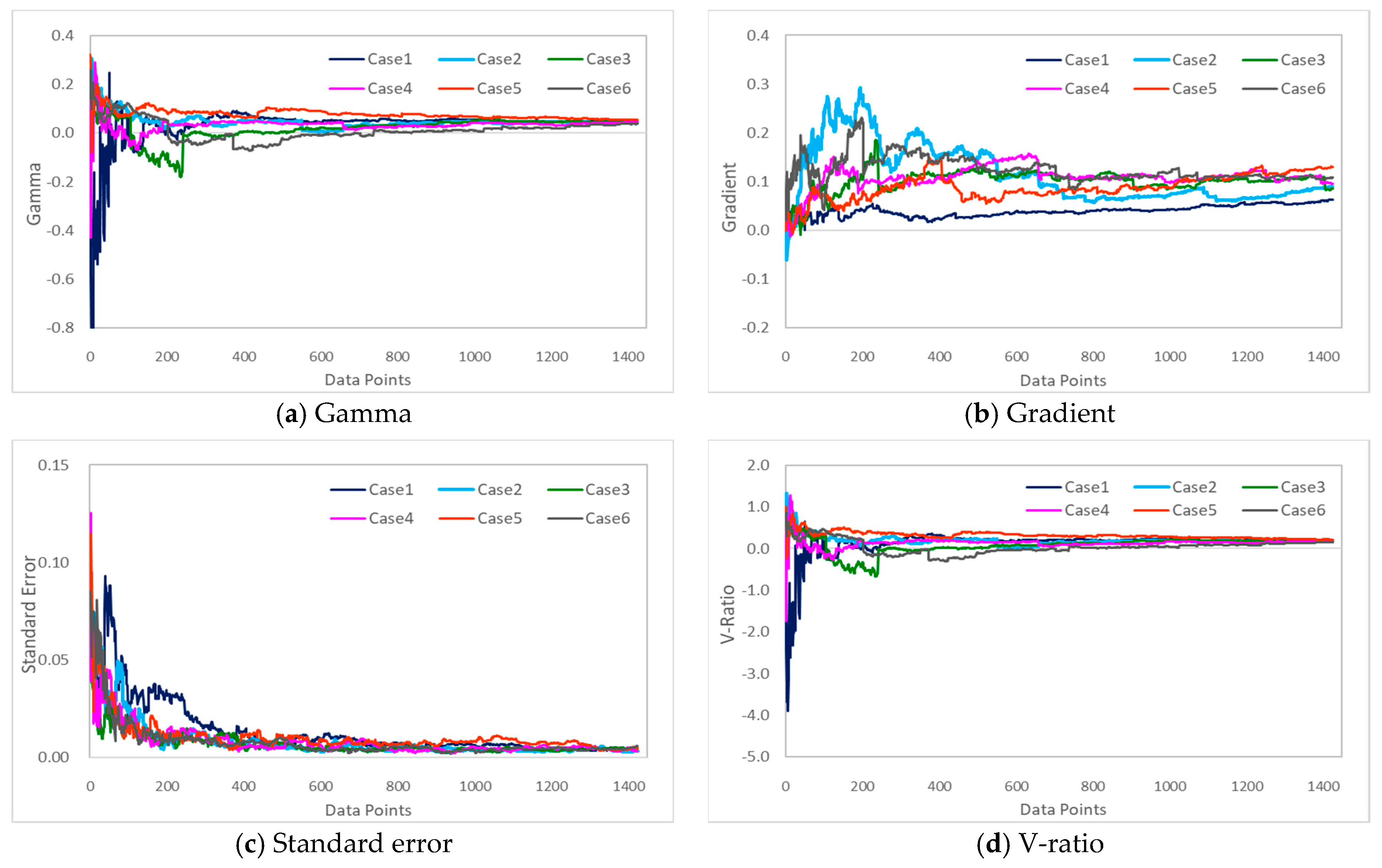
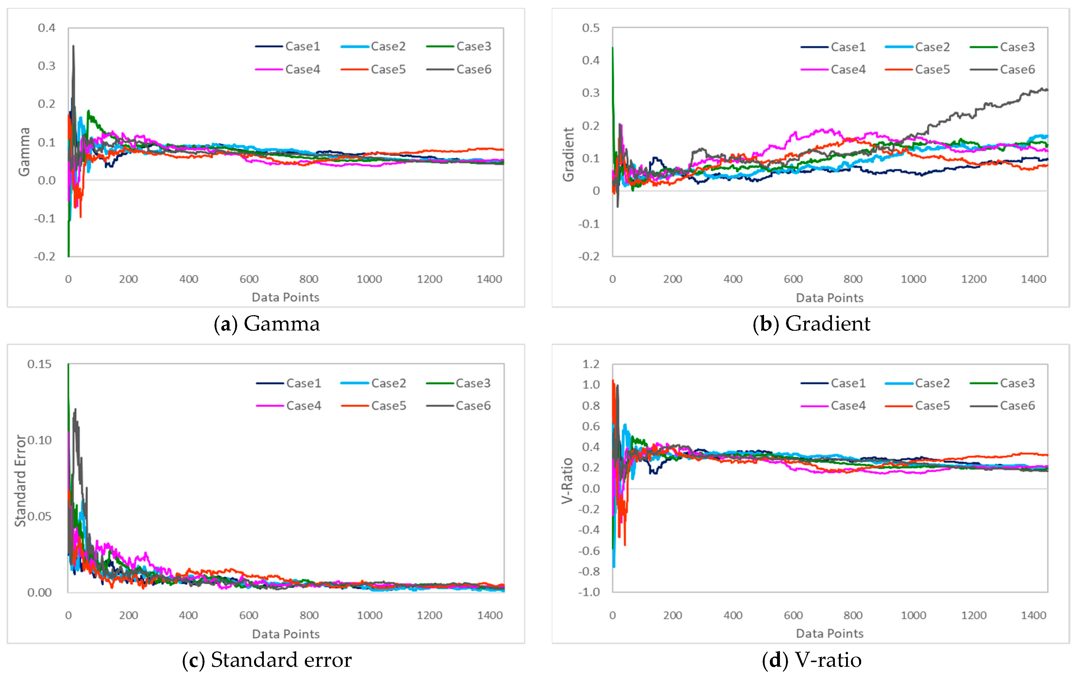
A Gamma test was performed to analyze the correlations between the input and output variables to select the optimal input data combination that shortened the simulation time, while increasing the accuracy of the data-driven model.

A Gamma Test is used to estimate the least mean square error calculated when modeling the data using a continuous nonlinear method. First published by Agalbjorn et al. [18], the technique has been advanced and established by many researchers [19]. The basic concept of the Gamma Test differs from conventional preprocessing data analyses using nonlinear methods. The analysis is performed under the assumption that the data are prepared as shown in Equation (2).

$$(x_i,y_i),1\le i\le M.$$

(2)

Here, the input vector $x_i\in R_n$ is limited to the closed set $C\in R_n$, and the output $y_i\in R_n$, which corresponds to the result of the general model or the dependent variable, is scalar. Vector $x$ affects the output value $y$ and is the independent variable that can be used as the input for prediction. The basic assumption for the relationship between $x$ and $y$ is as follows:

$$y=f\left(x_1\cdots \cdots x_m\right)+r.$$

(3)

Here, $f$ is an exponential smoothing function and $y$ is a probability variable indicating noise. In Equation (3), the $x$ value represents the input data, and the $y$ value represents the prediction (target value). The Gamma Test performs a nonlinear analysis based on the kth $\left(1\le i\le p\right)$ closest variable $N\left[i,k\right]$ for each vector $x_i\left(1\le i\le M\right)$. For each input data $x$, the mean square root distance to the $k$ closest neighbor data is calculated. This is shown in Equation (4). The mean square root distance with the $k$ closest neighbor data is also calculated using the same method for y, which is the result (or target) value for the independent variable, x (Equation (5)).

$${\delta }_M\left(k\right)=\frac{1}{M}{\displaystyle \sum }_{i=1}^M{\left|x_{N\left(i,k\right)}-x_i\right|}^2\left(1\le k\le p\right),$$

(4)

$${\gamma }_M\left(k\right)=\frac{1}{2M}{\displaystyle \sum }_{i=1}^M{\left(y_{N\left[i,k\right]}-y_i\right)}^2\left(1\le \mathrm{k}\le p\right).$$

(5)

When the relationship with the physical distance to the closest neighbor data is calculated for each variable, the same number of $\delta$ and $\gamma$ values as the number of data are generated, and a regression equation is derived to calculate $\tau$ from these two variables. The gamma statistic $\tau$ is an estimate of the variance of the ANN’s result that cannot be explained by the exponential smoothing data model.

$$\gamma =A\delta +\tau$$

(6)

$$V_{ratio}=\frac{\tau }{{\sigma }^{2\left(y\right)}}$$

(7)

Here, $\tau$ is used to calculate the $V_{ratio}$ uncertainty index according to a specific combination of input data. In Equation (7), ${\sigma }^{2\left(y\right)}$ is the variance of output $y$, which makes it possible to judge the predictability of the output in terms of whether it can be modeled smoothly and reliably, independent of the output range. A $V_{ratio}$ value close to 0 indicates a high predictability of the output $y$. The above process can help determine the amount of data required to build a model with a mean square error that approximates the expected noise variance [20].

2.5. Data-Driven Model (Adaptive Neuro-Fuzzy Inference System; ANFIS)

This study applied the ANFIS model, developed using the neuro-fuzzy model theory combining an ANN with fuzzy theory, which is appropriate for nonlinear prediction and simplifying the complex relationships of the numerous input variables. The ANFIS model has been applied in various fields to combine the advantages of the neural network and fuzzy theory, while minimizing the disadvantages.

Neural networks have an excellent data-based processing ability because of their large flexibility in system configuration. In contrast, fuzzy theory is appropriate for processing and inferring ambiguous information within a logical system. However, membership functions and rules need to be determined through trial and error, and repeated readjustment of the processes is required to build the desired fuzzy theory system [3].

A neuro-fuzzy model has been proposed to solve these issues. This model automatically adjusts the membership functions and rules in accordance with the control object using the input and output information obtained from the control environment with the structure and learning ability of the neural network. Determining the membership function for fuzzy inference using a neural network has the following advantages [3]:

• Because the membership function is determined by the learning of the neural network instead of the user’s subjective judgment, trial and error and readjustment processes can be omitted, thus shortening the system construction time.
• The neural network is nonlinear; thus, the accuracy of the results can be improved by selecting a nonlinear membership function to represent the relationships of nonlinear input and output data.
• The rules can be automatically obtained using the learning function of the neural network.

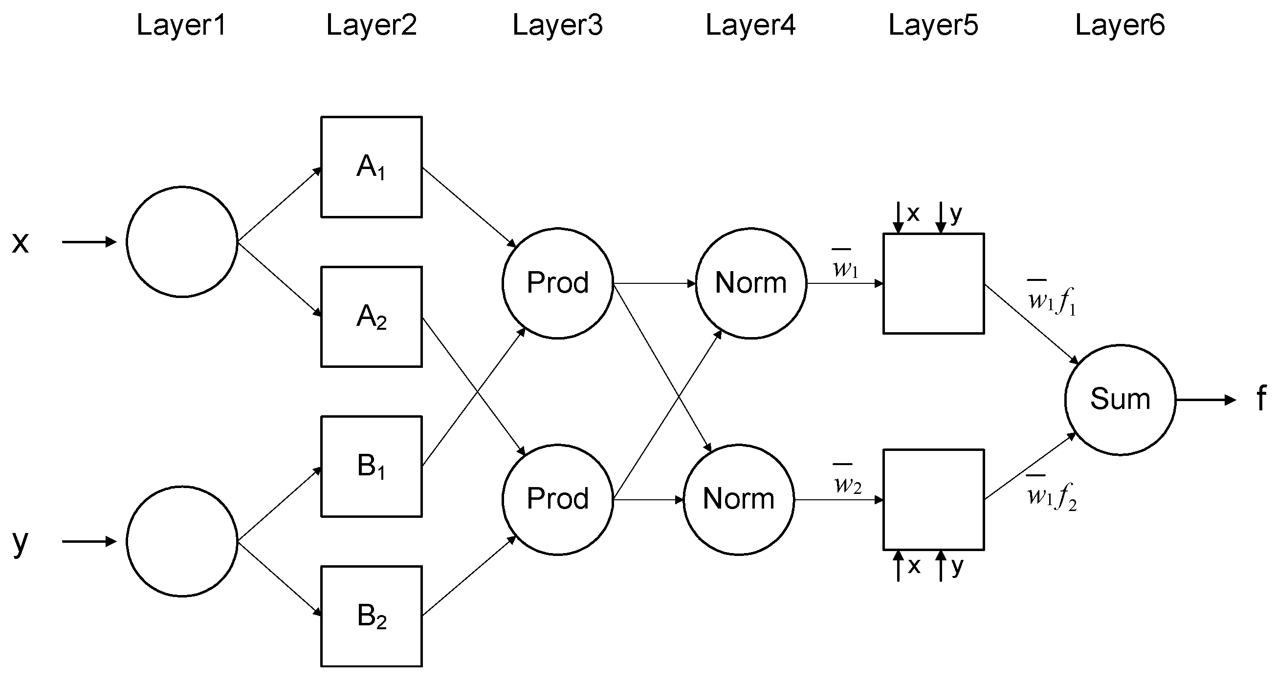
The neuro-fuzzy structure is composed of five layers with a node output in each layer. Layer 1 is an input node and Layer 2 is an adaptive node, and they act as a membership function. Layer 3 is a fixed node indicated as Prod, and the output of each node represents the connection strength. Layer 4 is a fixed node indicated as Norm, and the output represents the normalized connection strength. Layer 5 calculates the weighted value of the output of the previous layer. Layer 6 is represented as the sum of all input signals to calculate the inference result for the entire system (Figure 4).

We applied the subtractive clustering algorithm for the fuzzy clustering technique in the neuro-fuzzy model. This algorithm assumes that each data point is a potential cluster center and uses the density of object data to determine the object data closest to the cluster center to define the representative cluster center; therefore, it has a high application potential.

In addition, data with low Epochs error values were selected as the parameters through the trial-and-error method, and included the range of influence, squash factor, accept ratio, and reject ratio.

2.6. Composition of Training Data for ANFIS Model Application

The data-driven model must be trained by a combination of variables that have a high correlation with the target variable to predict the target outputs. Thus, this study selected BOD as the target variable for predicting water quality. With regard to the input variables, the discharges of the Seomjin River Dam (Unam and Chilbo), Sanseong water intake, Nakyang Weir water intake (Gimje and Jeongeup irrigation canals), rainfall, and flow rate (t), and the input variables of one day before (t − 1) and one day after (t + 1) were used. These input variables were selected considering the usability of the data-driven model because the corresponding observation data were generated every day, and when they were input into the data-driven model, the water quality (BOD) for Dongjin River 3 point could be predicted without running the HSPF model. A gamma test was performed first to determine which composition of input variables could improve the ability to predict BOD, and thus, the optimal combination of input variables was determined.

The ANFIS model, which was constructed through training, verification, and testing, was employed in this study. The parameters of the membership function were determined through the training and verification processes. As the parameter values of the membership function change based on the conditions used in this process, the results of the ANFIS model also vary. The ANFIS model was built for irrigation and non-irrigation periods, as the target watershed is highly affected by agricultural water intake because of its large irrigation system. To split the input data for learning, the specified indices method, which best reflected the time-series data, was used among the random indices method, blocks of indices method, specified indices method, and interleaved indices method [21].

3. Results and Discussion

3.1. HSPF Model Calibration and Verification Results

3.1.1. Flow Rate

Model calibration refers to the process of configuring the initial conditions and parameters of the model, in accordance with the actual conditions and estimating the parameter values that can generate simulated values closest to the observed values [22]. The trial-and-error method was used to make the simulation result of the model as close as possible to the observed values for the calibration period. By performing the verification, the model parameters adjusted during the calibration period were validated.

The coefficient of determination (R²) and percent (%) difference were calculated as mentioned in the previous section. As shown in

Table 5. Calibration and verification results of the flow rate in the Dongjin River Basin.

Gauging Station	Calibration		Valification
	R2	% Difference	R2	% Difference
Haengjeonggyo	0.97	1.05	0.89	10.03
Jeongugyo	0.80	4.37	0.86	10.82
Chogangri	0.85	12.51	0.91	14.32

, the results were very good, indicating that the simulated values of the model reflected the measured values very well for all three gauging stations. Figure 5 shows the calibration and validation results for the Jeongugyo gauging station located in the main Dongjin River as the representative station. Most of the simulated peak values during the rainfall events were slightly smaller than the observed values, indicating that the simulation reproduced the flow rate during the dry and low flow seasons more accurately.

3.1.2. Water Quality

The HSPF model was first calibrated for water temperature and DO, and then for BOD, TN, TP, TOC, and Chl-a. In this study, only the results of BOD, the indicator used for predicting water quality, are presented. In the calibration and validation results for BOD, the percentage (%) difference values were all 15 or lower, indicating “very good” results. The RMSE values, which are close to zero if the simulated and measured values are identical, were 1.35 and 1.65, respectively (

Table 6. Calibration and verification results of BOD at Dongjingang 3 (Dongjin A).

Year	Mean OBS	Mean SIM	% Diff	RMSE	Criteria
Calibration (16–18 y)	2.9	2.8	4.37	1.65	0.96 (very good)
Verification (13–15 y)	2.6	2.3	10.8	1.35	0.89 (very good)

, Figure 6). The concentration ratio for the averages of the measured and simulated values was also within the confidence range (0.71–1.06), and the simulated values reflected the trend of the observation values well, as shown in Figure 5. Considering the complex water quality mechanisms and the various spatial characteristics of the watershed, the overall simulation was performed sufficiently during the simulation period.

3.2. Prediction of Water Quality Using the Data-Driven Model

3.2.1. Selection of Optimal Input Variables

To consider the correlations between the input and output variables before building the ANFIS model for BOD prediction, as described in Section 2.6, a combination of various input variables was selected (

Table 7. Combination of input variables.

Case	Input Data			Target
	Discharge and Intake	Flow Rate (Jeongugyo)	Rainfall
1	Seomjin River Dam discharge (Unam waterway, Dongjin waterway), water intake (Nakyang weir, Sanseong)	Q(t), Q(t − 1), Q(t + 1)	R(t), R(t − 1), R(t + 1)	BOD
2		Q(t), Q(t − 1), Q(t + 1)	R(t)
3		Q(t), Q(t − 1)	R(t), R(t − 1)
4		Q(t)	R(t), R(t − 1), R(t + 1)
5		-	R(t), R(t − 1), R(t + 1)
6		Q(t), Q(t − 1), Q(t + 1)	-

). The results of the gamma test include gamma, gradient, standard error, and V-ratio. A larger gamma value indicates a low correlation between the data and a high uncertainty. The standard error indicates the standard deviation of the data. A gradient closer to 0 indicates a higher BOD predictability based on the input data [23]. The results of the gamma tests for irrigation and non-irrigation periods are outlined in

Table 8. Averages of the gamma test results (irrigation period).

Case	Input Data				Ranking
	Gamma	Gradient	Standard Error	V-Ratio
1	0.032481	0.039864	0.013330	0.126649	-
2	0.047462	0.113928	0.008299	0.195536	4
3	0.019416	0.101115	0.007077	0.080209	2
4	0.033563	0.109131	0.008234	0.137404	3
5	0.077909	0.088863	0.010356	0.319419	5
6	0.011280	0.124402	0.007989	0.041198	1

and

Table 9. Averages of the gamma test results (non-irrigation period).

Case	Input Data				Ranking
	Gamma	Gradient	Standard Error	V-Ratio
1	0.072242	0.062415	0.006974	0.283613	-
2	0.070719	0.088788	0.007914	0.279658	5
3	0.070464	0.103065	0.009455	0.257889	4
4	0.062585	0.124396	0.010028	0.230381	1
5	0.064329	0.092028	0.008816	0.267492	2
6	0.068359	0.144772	0.010034	0.272255	3

. Cases with a ranking closer to 1 can provide better prediction owing to the lower uncertainty of the combination of input variables. In Case 1, all the data were excluded from the ranking to measure uncertainty according to the selected combination of hydrological conditions of the Dongjin River, and unnecessary variables were removed. The results showed that during the irrigation period, Case 6, which did not use rainfall, showed the lowest gamma value and V-ratio, with a ranking of 1. In the non-irrigation period, Case 4 was ranked 1, and the rainfall condition had a greater effect on the BOD than that during the irrigation period when the amount of discharge flowing into the Seomjin River Dam was constant. This implies that a more stable result can be obtained from the data-driven model using the combination in Case 6 for the irrigation period and the combination in Case 4 for the non-irrigation period. The variability of gamma, gradient, standard error, and V-ratio according to the length of each input data combination is shown in Figure 7 and Figure 8, which visually show the uncertainty relative to the quantity of data used.

3.2.2. BOD Prediction Result for the Dongjin River Basin

The BOD was predicted by inputting data from 2018 to the data-driven model (ANFIS) constructed using the datasets in Cases 6 and 4 for the irrigation and non-irrigation periods, respectively (Figure 9,

Table 10. BOD prediction results at Dongjingang 3 (Dongjin A).

BOD (2018)	R2	% Diff	RMSE	Mean HSPF	Mean ANFIS
Irrigation period	0.84	1.48	0.57	4.4	4.4
Non-irrigation period	0.84	0.70	0.33	2.2	2.2

). These results were compared with the simulated values from the calibrated and validated HSPF model. In the irrigation period, R² was 0.84, the percent difference was 1.48, and the RMSE was 0.57. In the non-irrigation period, R² was 0.84, the percent difference was 0.70, and the RMSE was 0.33.

For additional validation of the ANFIS model, the amount of discharge, water intake, precipitation, and flow data from the water level observation for 2019 were collected, entered into the ANFIS model, and compared with the data for the eight-day interval observation at the Dongjin A location (Figure 10,

Table 11. BOD prediction results at Dongjingang 3 (Dongjin A).

BOD(2019)	R2	% Diff	RMSE	Mean OBS	Mean ANFIS
Irrigation period	0.88	1.73	4.79	4.4	4.5
Non-irrigation period	0.90	1.61	0.13	2.2	2.3

). For the irrigation period, R² was 0.88, the percent difference was 1.73, and the RMSE was 4.79. For the non-irrigation period, R² was 0.90, the percent difference was 1.61, and the RMSE was 0.13. Thus, the model effectively predicted both the irrigation and non-irrigation periods.

The data-driven model developed in this study showed an excellent predictive performance for the BOD at the targeted river management points of the Dongjin River. These points were those designated for TMDL monitoring and target water quality management in Korea. Our results confirm that it is possible to predict water quality under various hydrological conditions on a more scientific basis, especially in a watershed highly affected by a large irrigation system.

To predict the water quality using a physics-based model, regularly adding input data (hourly meteorological data, geospatial data, the pollutant load data, hydrological conditions, etc.) to run the model is necessary. In addition, processing the input data, which is suitable for the model, and running the model consumes time.

However, the use of the daily observation data as input variables in the ANFIS model developed in this study increased the reliability and convenience of prediction of the water quality under various hydrological conditions, without running the physics-based model.

4. Conclusions

Big-data-based analysis techniques are being used for watershed management. Among them, predictive analytics aim to construct future analysis and prediction functions through the identification of past patterns using a physics-based model. Moreover, predictive analytics can be used to develop a data-driven model using an ANN trained with past observation data. The models can then be applied to develop sufficient and sustainable water management strategies to mitigate the negative effects associated with water disasters such as floods and water quality pollution [24]. Predicting water quality with a physics-based model can provide more accurate results. However, the pre- and post-processing of the model can be time-consuming. This study derived water quality data under various hydrological conditions for approximately 10 years for the target watershed from a physics-based model, which was then used as the basis for constructing a data-driven model, thus presenting a highly reliable and fast water quality prediction method using simple input data.

First, the HSPF model was built by inputting available watershed environmental conditions, including geospatial data, meteorological data, hydrological conditions, and the pollutant load of the Dongjin River Basin. Then, the BOD values were obtained under various hydrological conditions through calibration and validation processes based on the observed values. To predict the BOD values using the data-driven model at the Dongjin River 3 (Dongjin A) station, the target water quality evaluation point of the Dongjin River Basin, the Seomjin River Dam discharges (Unam and Chilbo), Sanseong water intake, Nakyang Weir water intake (Gimje and Jeongeup irrigation canals), rainfall, and flow rate at the gauging station were selected as the input variables. These variables were chosen considering the usability of the data-driven model as they are measured daily. When they were input into the data-driven model, the BOD values for the Dongjin River target station could be predicted without running the HSPF model.

A Gamma Test was performed to improve the BOD prediction efficiency before building the data-driven model (ANFIS), and the optimal combination of input variables was derived separately for the irrigation period (April–September) and the non-irrigation period (October–March). Consequently, the most appropriate combination was the Seomjin River Dam discharge, Sanseong water intake, Nakyang Weir water intake, and flow rates at the Jeongugyo gauging station for the irrigation period. For the non-irrigation period, the additional rainfall was analyzed to be appropriate.

The ANFIS model simulation results showed an excellent predictive performance for both the irrigation and non-irrigation periods.

The proposed BOD prediction model minimizes the time required to predict water quality, while using fewer variables, and provides more efficient and reliable results. Thus, the model will serve as an essential tool for the decision-makers who manage the intake of agricultural weirs in determining the water quality of the main river in the Dongjin River Basin.

The model built in this study is a data-driven model that uses the results of the verified HSPF model as training data in place of insufficient water quality observation data. Therefore, for a more accurate water quality prediction, the data-driven model needs to be upgraded through continuous calibration of the HSPF model and periodic training. In the future, higher amounts of representative water quality data for the Dongjin River will enable the development of a more reliable data-driven model.