Forecasting of Significant Wave Height Based on Gated Recurrent Unit Network in the Taiwan Strait and Its Adjacent Waters

Abstract

Significant wave height (SWH) forecasting is a key process for offshore and costal engineering. However, accurate prediction of the SWH is quite challenging due to the randomness and fluctuation features of waves. This paper employs a novel deep learning method, the gated recurrent unit network (GRU), to forecast SWH with lead times of 3, 6, 12 and 24 h. The data sets used in this study include the wind speed of the past 3 h and the current SWH as inputs, which were obtained from six buoy stations in the Taiwan Strait and its adjacent waters. The GRU results are compared with those of back propagation neural network (BP), extreme learning machine (ELM), support vector machine (SVM), and random forest (RF). Although the error indices of the six stations are different, the general performance of GRU is satisfactory, with a faster forecasting speed, smaller volatility and better adaptability. Using buoy station 46714D as an example, the root mean square error (RMSE) predicted by GRU reaches 0.234, 0.299, 0.371, and 0.479 with lead times of 3, 6, 12, and 24 h, respectively.

1. Introduction

Marine disasters pose a severe threat to many countries in the world, leading to tremendous casualties and economic losses. To this end, investigating the characteristics of ocean waves, especially the significant wave height (SWH), is of pivotal importance to maritime activities and coastal engineering. An accurate and reliable prediction of SWH contributes to the smooth progress of activities such as fisheries, marine resources exploitation, safe navigation, and construction and maintenance of coastal structures [1,2]. However, the irregularity of ocean waves presents great challenges in predicting SWH.

In general, there are three mainstream approaches to predict SWH, including empirical, numerical and machine learning methods. The classical empirical-based models such as auto regressive moving average (ARMA) have been long established, but they have a limited ability to capture the non-stationarities and non-linearity in data series [3]. In the past decades, a number of researchers have sought to predict SWH using physics-based models, which rely primarily on a form of the spectral energy or action balance equation. Although numerical models have proven to be effective in wave height prediction over a large spatial and temporal range, their drawbacks have also been noted, and the cost of computational resources and time is extremely high, especially for the calculations of a higher resolution grid in the nearshore zones where the seabed topography is intricate [4,5].

The increasingly rapid advances in machine learning have triggered a huge amount of innovative inquiries in SWH prediction. Machine learning methods use statistics to gain a deeper insight into the spatial and temporal link hidden in the historical time series.

Zamani et al. [6] conducted a detailed study of several data-driven models based on artificial neural networks (ANNs) and instance-based learning (IBL). Experiments showed that the ANNs have a slight superiority over IBL, and ANNs also exhibit competitive advantages in predicting extreme wave conditions. The predictive capability of several machine learning approaches including support vector machine (SVM), Bayesian network (BN), ANN and adaptive neuro-fuzzy inference system has been inspected by Malekmohamadi et al. [7]. The results manifested that the behavior of these models are acceptable except the results of BN. By incorporating a genetic algorithm with Kalman filtering, Altunkaynak and Wang [8] developed a new technique to predict SWH. The superiority of this method over ANN was shown by its lower mean relative error and mean square error. Nitsure et al. [9] applied genetic programming to predict wave heights using wind information as an input. The prediction results with lead times up to 12 h and 24 h were satisfactory, where the coefficients of correlation between the predicted and measured values were higher than 0.87. Prahlada and Deka [10] strived to present a hybrid model of wavelet and an artificial neural network for SWH prediction across multistep lead time by combining the beneficial qualities of both. The presented method has been proven to be effective and feasible. Cornejo-Bueno et al. [11] proposed a hybrid grouping genetic algorithm–extreme learning machine approach for marine energy applications in SWH and flux prediction and obtained desirable results. Nikoo et al. [12] conducted SWH prediction based on a fuzzy K-nearest neighbor (FKNN) model where the variation of wind direction will affect the fetch length. The prediction results of FKNN outperformed those obtained by BN, regression tree induction and support vector regression, especially in the prediction of wave heights larger than 2 m. Wei and Hsieh [13] adopted ANN in two distinct situations to assess the practicability of predicting waves using the data gathered from the adjacent buoy. The study showed that the model involving information from the adjacent buoy outperforms the one without extra data. Considering the edges of back propagation neural networks (BP) and cuckoo search algorithms (CS), Yang et al. [14] creatively attempted to predict SWH based on a CS–BP model, and the proposed model offers promising potential for wave height prediction. A recent study carried out by Zhang and Dai [15] involved the conditional restricted Boltzmann machine in the classical deep belief network to predict SWH. The measurement criterion revealed that the newly proposed method has a strong ability for short-term and extreme events prediction.

More recently, the long short-term memory network (LSTM) [16], which is an improved form of a recurrent neural network (RNN), has been attracting considerable interests. Son et al. [17] found a novel perspective to predict real-valued SWH from a series of sequential ocean images using the bi-directional convolutional LSTM model, and low error indices were obtained. Fan et al. [18] employed LSTM to predict SWH for various forecasting time horizons with higher accuracy, and proposed a simulating waves nearshore-LSTM to make a single-point prediction. A great deal of previous research into SWH prediction has focused on using all kinds of shallow machine learning models such as BP, SVM and so on, but they have failed to completely exploit the inner correlations between historical information over the long term. LSTM has been successfully utilized to predict SWH. However, a conspicuous shortcoming with LSTM is that it entails a large number of parameters for training. Consequently, the training process is time consuming and it easily becomes overfitted.

The gated recurrent unit network (GRU) is optimized and condensed on the basis of LSTM, which has two gates named reset gate and update gate to control the flow of information. Benefiting from the structure, the forecasting speed of GRU is effectively improved and maintain the strength of LSTM at the same time [19]. GRU has emerged as a powerful tool in various applications encompassing time series prediction, such as machine health monitoring [20,21], wind speed prediction [22,23,24], and traffic flow prediction [25,26].

Nevertheless, to the authors’ cognition, there has been very little research that seeks to predict SWH using the novel deep learning method GRU over a large range and long prediction interval. Therefore, the prospective study sets out to predict SWH based on GRU at six buoy stations in the Taiwan Strait and its adjacent waters, and compare the prediction results of GRU with those obtained by BP, extreme learning machine (ELM), SVM, and random forest (RF).

The overall structure of this essay takes the form of five parts. The second part describes the study materials used in this study. The third part gives an explanation of the gated recurrent unit network and the evaluation indicator. The following part presents the obtained results, along with discussions. The final part gives a summary of the work.

2. Materials

The Taiwan Strait is China’s largest strait connecting the East China Sea and the South China Sea, which is not only an important maritime area for historical trade routes, but also a strategic point of modern geopolitics. Therefore, it enjoys a high reputation as the “sea corridor”. The topography of the Taiwan Strait is violently undulant; it is wide in the south, narrow in the north and shaped like a horn, and brings about the prominent narrow tube effect. As the frequency of production activities and shipping in this area is constantly increasing, there is an urgent need to make timely and accurate wave forecasting in this strait.

To test the performance of GRU, six buoy stations distributed at different sites in the Taiwan Strait and its adjacent waters were selected. The hourly data used for SWH prediction is owned and maintained by the National Marine Data Center (http://mds.nmdis.org.cn/) and the European Marine Observation and Data Network (http://www.emodnet-physics.eu/map/).

Table 1. Details of the selected stations.

Buoy ID	Latitude (°N)	Longitude (°E)	Water Depth (m)	Period of Data	Max SWH (m)	Max Wind Speed (m/s)	The Number of Data
46714D	22.31	120.35	110	14 Septmber 2012–10 August 2015	8.4	30.2	22,149
46735A	23.72	119.55	14	14 Septmber 2012–3 February 2017	5.9	21.6	31,699
46787A	24.38	118.41	16	14 Septmber 2012–31 December 2015,	5.2	17.5	26,091
C6V27	21.02	118.86	2623	12 Septmber 2012–2 December 2016	13.4	27.7	26,415
C6W08	26.38	120.54	55	14 Septmber 2012–13 December 2015,	12.8	24.4	26,601
NanJi	27.5	121.1	23	1 January 2015–30 November 2016,	6.5	27.5	16,677

gives details of the selected stations, including the exact locations, water depth, the period of data, the maximum SWH and wind speed during the corresponding period of each buoy station and the total number of available data. Figure 1 displays the distributions and water depth of the selected stations.

The key part of wind–wave forecasting is to predict SWH with lead times of a few hours or days using the historical information. According to [27], wind speed has been identified as a major contributing factor to the generation of waves. Furthermore, the previous SWH also exerts a dominant effect due to the continuity of waves. Therefore, the available previous observations of wind speed and SWH are fed into the model as inputs.

In this study, 80% of the available data were utilized for training the model, and the remaining 20% were used for testing.

3. Methodology

3.1. Wave Forecast Model

Since traditional neural networks are transmitted through full connection and each node in the same layer is not connected, they may fail when dealing with the temporal problems.

In this context, RNN has been proven to be more powerful in extracting temporal patterns than traditional neural networks by building self-loop connections from a node to itself and sharing parameters across different time steps.

The standard RNN take their input from the current input $x_t$ along with what they have picked up previously.

Firstly, the hidden state $h_t$ carrying the network memory can be computed by

$$h_t=f\left(W{h}_{t-1}+U{x}_t+b\right)$$

(1)

where $h_{t-1}$ is the previous hidden state; $x_t$ is the new input; $W$ and $U$ are the weight matrices; $b$ is the bias vector and $f$ is a nonlinear activation function. Then the current state $o_t$ is calculated as

$$o_t=W_o{h}_t+b_o$$

(2)

where $W_o$ is the weight matrix, and $b_o$ is the bias vector.

Although RNN exhibits a robust capability of modeling nonlinear time series in an effective fashion, it cannot escape the vanishing gradient and exploding gradient problems, and its accuracy decreases when the time span becomes longer.

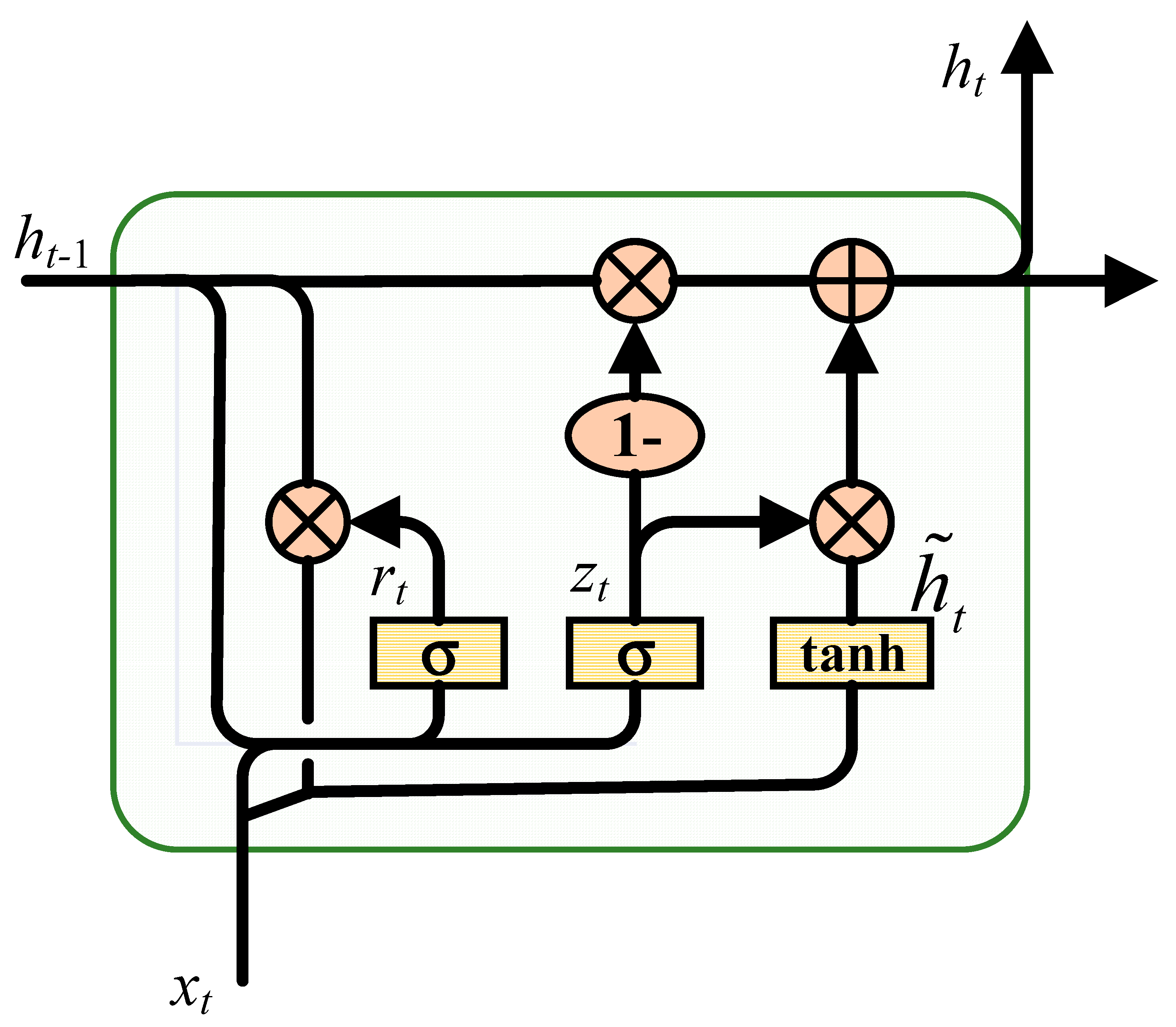
A long short-term memory network (LSTM) was proposed to mitigate the aforementioned problems, but the time consuming training process may hinder a wide-spread adoption of LSTM in real-time and fast SWH forecasting. In our paper, we employ another notable RNN variant, a gated recurrent unit network (GRU). Figure 2 shows the inner structure of the GRU.

Both RNN and GRU have chain-like modules, but the repeating modules of GRU are more complicated. Each repeating module of GRU contains two gates, named update gate and reset gate, which gives GRU the ability to control the flow of information. The two gates are sigmoid units that map the variables in $\left[0,1\right]$, where the value between 0 and 1 is the ratio of memory. Thus, GRU can tackle the correlation with the time series over long and short terms.

Firstly, the reset gate $r_t$ controls how much information from the previous hidden state will be carried over to the current hidden state, where

$$r_t=\sigma \left(W_r·\left[h_{t-1},x_t\right]+b_r\right)$$

(3)

The new memory candidate ${\tilde{h}}_t$ is produced by $r_t$ with a tanh layer, which derives from the following:

$${\tilde{h}}_t=\tanh \left(W·\left[r_t·h_{t-1},x_t\right]\right)$$

(4)

The update gate $z_t$ determines whether the hidden state will be updated with a new hidden state, where

$$z_t=\sigma \left(W_z\left[h_{t-1},x_t\right]+b_z\right)$$

(5)

In the end, the hidden state $h_t$ is renewed by

$$h_t=\left(1-z_t\right)·h_{t-1}+z_t·{\tilde{h}}_t$$

(6)

In Equation (3) to Equation (6), $W_r$, $W_z$ are the weight matrices, $b_r$, $b_z$ are the corresponding bias vectors.

3.2. Data Preprocessing and Evaluation Criteria

In order to keep all the variables on the same scale and guarantee a stable convergence in the model developed in the present study, the following standardization formula is used

$$x\prime =\frac{x-\mu }{{\delta }^2}$$

(7)

where $\mu$ represents the mean, and $\delta$ represents the variance of data.

For the quantitative evaluation of the model’s performance, three statistical metrics, the root mean square error (RMSE), coefficient of correlation (R) and index of agreement (IA), are considered:

$$\mathrm{RMSE}=\sqrt{\frac{1}{n}{\displaystyle \sum _{i=1}^n{\left(x_i-y_i\right)}^2}}$$

(8)

$$\mathrm{R}=\frac{{\displaystyle \sum _{i=1}^n\left(x_i-\overline{x}\right)\left(y_i-\overline{y}\right)}}{\sqrt{{\displaystyle \sum _{i=1}^n{\left(x_i-\overline{x}\right)}^2{\displaystyle \sum _{i=1}^n{\left(y_i-\overline{y}\right)}^2}}}}$$

(9)

$$\mathrm{IA}=1-\frac{{\displaystyle \sum _{i=1}^n{\left(y_i-x_i\right)}^2}}{{\displaystyle \sum _{i=1}^n{\left(\left|y_i-\overline{y}\right|+\left|x_i-\overline{x}\right|\right)}^2}}$$

(10)

where $x_i$ is the observed value at the $i\mathrm{th}$ time, $y_i$ is the predicted value at the same moment, $n$ is the number of time steps, $\overline{x}$ is the mean of observed data, and $\overline{y}$ is the mean value of predicted values.

4. Results and Discussions

According to the theory that a wave is generated by wind interacting with the ocean surface, the current SWH together with wind speed over the past three hours are imposed as input variables to predict SWH using GRU for various forecasting time horizons. The experiments of four widely used machine learning algorithms, BP, ELM, SVM and RF, were conducted for comparison.

The parameters of GRU were set by means of trial and error, while the parameters of the other four methods were selected according to the previous study. The experiments showed that excessive model parameters may bring about a time consuming training process without significant improvements on the prediction effectiveness. Therefore, the parameter setting should be balanced against the prediction performance and the time consumption.

Table 2. Parameter settings of the five algorithms.

Algorithm	Settings
GRU	m = 2, S = 64, g = 0.001, activation function is tanh, k = 200
BP	S = 5, g = 0.1, k = 100
RF	N = 100, maxdeep = 3
ELM	S = 30, activation function is sigmoid.
SVM	C = 1, $\epsilon =0.1$, the kernel function is Radial Basis Function.

lists the key model parameters of the five algorithms, where m is the number of hidden layers, S is the number of neurons in each hidden layer, g represents the learning rate, k stands for the number of training epochs, C is the penalty parameter, $\epsilon$ is the error tolerance, N is the number of trees in RF, and maxDeep is the maximum depth of each tree. In the following paper, the best results are highlighted with bold font.

4.1. SWH Prediction with Lead Times of 3 h

In this section, the current SWH and wind speed 3 h ago are fed as inputs to forecast SWH with lead times of 3 h.

The error indices of the five algorithms at six different stations selected from the Taiwan Strait and its adjacent waters are presented in

Table 3. Error indices of predicted SWH with lead times of 3 h.

Station	Algorithm	RMSE	R	IA
46714D	GRU	0.234	0.938	0.967
	SVM	0.411	0.929	0.886
	BP	0.254	0.931	0.965
	ELM	0.509	0.735	0.862
	RF	0.268	0.921	0.959
46735A	GRU	0.262	0.943	0.968
	SVM	0.443	0.934	0.888
	BP	0.274	0.936	0.966
	ELM	0.413	0.862	0.926
	RF	0.271	0.938	0.966
46787A	GRU	0.239	0.875	0.932
	SVM	0.361	0.860	0.789
	BP	0.244	0.870	0.928
	ELM	0.468	0.681	0.796
	RF	0.248	0.865	0.925
C6V27	GRU	0.349	0.947	0.972
	SVM	0.534	0.943	0.924
	BP	0.360	0.944	0.971
	ELM	0.601	0.862	0.924
	RF	0.370	0.940	0.969
C6W08	GRU	0.324	0.950	0.972
	SVM	0.549	0.945	0.902
	BP	0.363	0.936	0.964
	ELM	0.603	0.844	0.914
	RF	0.367	0.936	0.962
NanJi	GRU	0.193	0.950	0.973
	SVM	0.381	0.942	0.878
	BP	0.226	0.934	0.960
	ELM	0.389	0.809	0.899
	RF	0.197	0.947	0.972

. It is apparent that all the indicators of GRU are better than those of the other four algorithms. The ability of GRU in predicting SWH far outpaces the others, which may be due to the fact that GRU can take full advantage of the useful information from the previous states without the vanishing gradient and exploding gradient problems. What stands out in this table is that the performances of SVM and ELM are strikingly poorer than the others, which indicates that SVM and ELM are not good choices to predict SWH. At station C6W08, the RMSE of GRU is 46.3% lower than that of ELM, and the R and IA of GRU reach up to 0.950 and 0.972, whereas the same indices of ELM are only 0.844 and 0.914. With regard to BP, RF, and SVM, the performances of all of the six stations are inferior to those of GRU to a greater or lesser degree.

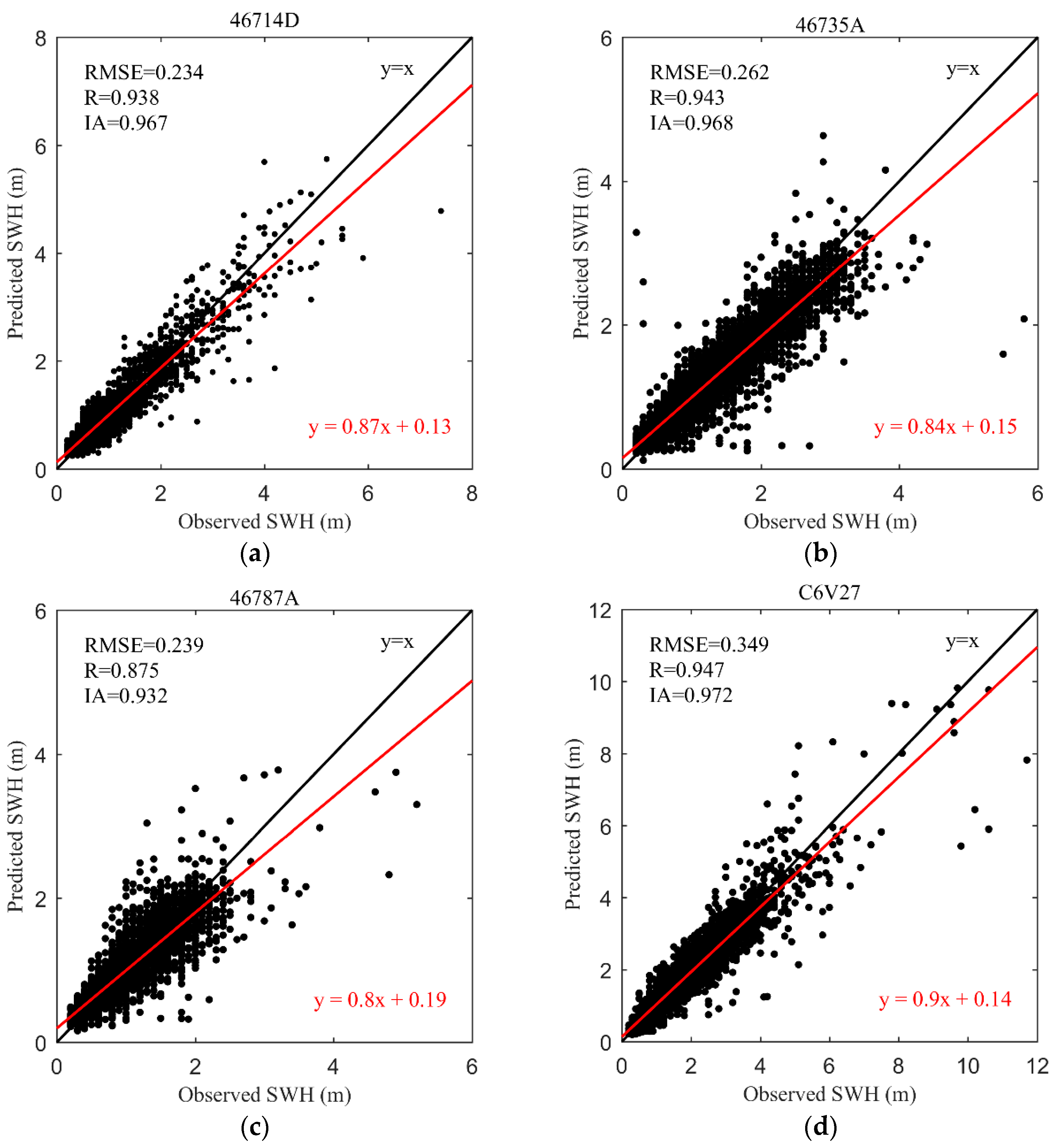
Figure 3 exhibits the scatter diagrams of the observed values and predicted SWH obtained by GRU with lead times of 3 h for the six stations.

As can be seen from Figure 3, the observed and predicted values produced by GRU have a considerable accordance for 3 hourly prediction. Especially at Station C6V27, the predicted SWH correlated very well with the observed values. Even so, what cannot be ignored is that there are some outliers that are not concentrated near the bisector. The most likely cause is that the vast majority of SWH observed at these stations are less than 4 m, whereas a few extreme events still exist.

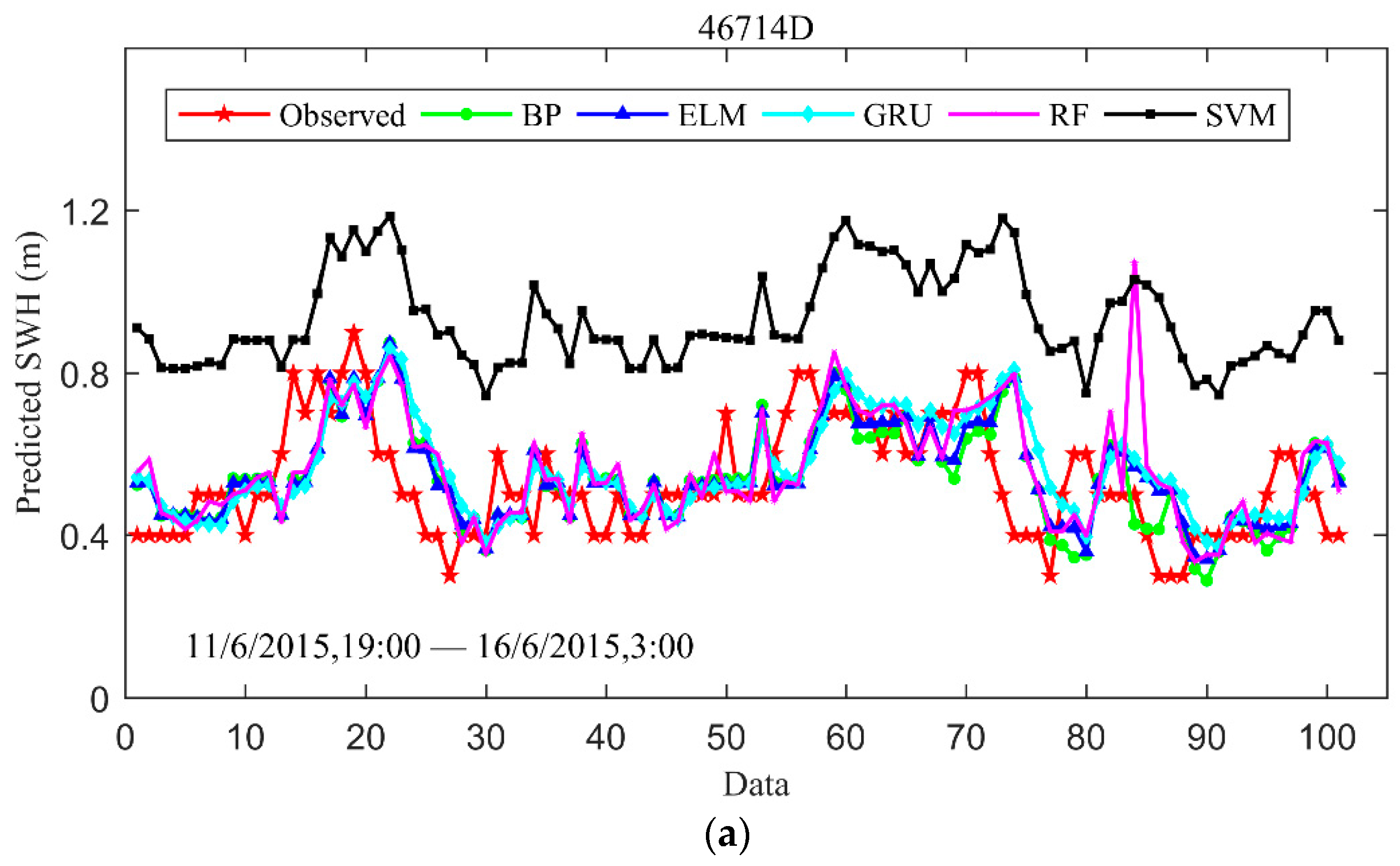
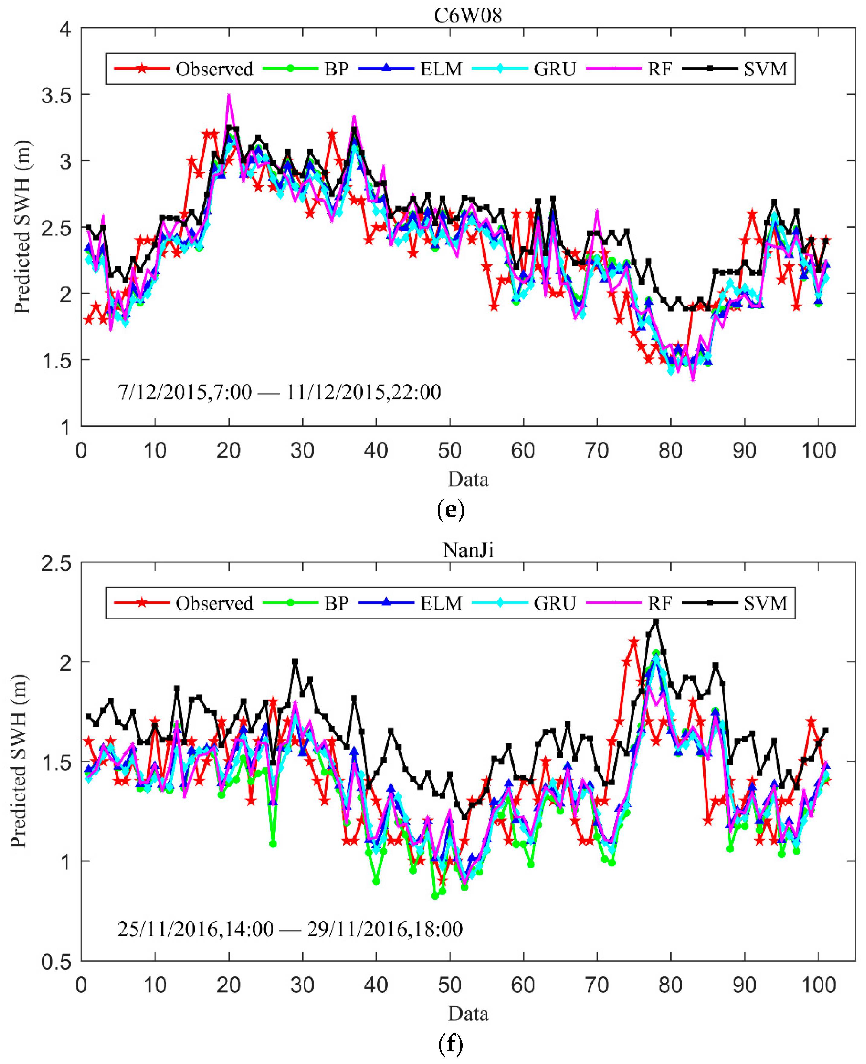
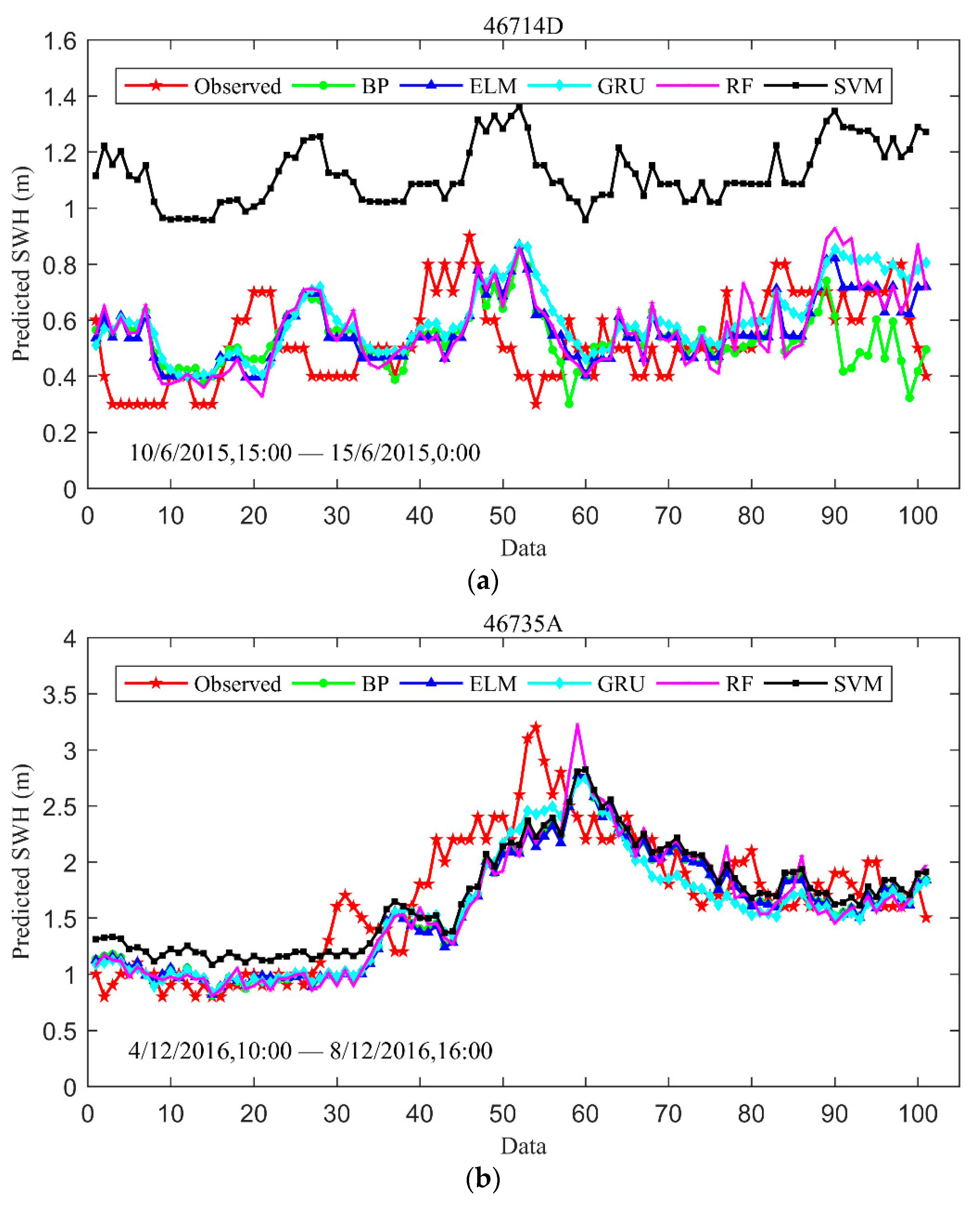
To reveal the difference in prediction performance between GRU and the other four methods clearly, we randomly choose a piece of the predictive results for each station to show in Figure 4, in which the number of data points is 100.

Given a closer inspection of Figure 4, it can be found that the test results of SVM and ELM tend to have larger volatility than GRU. One of the known reasons that bring out volatility is that ELM and SVM are more susceptible to parameter selection. In practical application, both of them are more likely to plunge into local minimum, so the stability is relatively poorer. By contrast, based on the gate mechanism, the reset gate throws away the unwanted information and the update gate propagates useful context from the previous hidden states, which endows GRU with a strong ability to exploit the future and previous information without sophisticated parameter tuning. Hence, the prediction made by GRU at all the selected stations with lead times of 3 h are of high accuracy and stability.

4.2. SWH Prediction with Lead Times of 6 h

The experiments with lead times up to 6 h are described in this section. A vertical comparison of Table 3,

Table 4. Error indices of predicted SWH with lead times of 6 h.

Station	Algorithm	RMSE	R	IA
46714D	GRU	0.299	0.899	0.943
	SVM	0.585	0.889	0.742
	BP	0.317	0.887	0.940
	ELM	0.655	0.597	0.780
	RF	0.329	0.880	0.936
46735A	GRU	0.340	0.901	0.943
	SVM	0.485	0.887	0.853
	BP	0.347	0.897	0.940
	ELM	0.467	0.811	0.897
	RF	0.349	0.895	0.940
46787A	GRU	0.301	0.792	0.875
	SVM	0.395	0.773	0.727
	BP	0.312	0.776	0.868
	ELM	0.567	0.484	0.665
	RF	0.314	0.773	0.866
C6V27	GRU	0.486	0.894	0.943
	SVM	0.656	0.889	0.873
	BP	0.497	0.889	0.937
	ELM	0.752	0.771	0.873
	RF	0.507	0.885	0.937
C6W08	GRU	0.453	0.899	0.941
	SVM	0.618	0.897	0.863
	BP	0.463	0.895	0.936
	ELM	0.726	0.764	0.867
	RF	0.498	0.876	0.924
NanJi	GRU	0.265	0.902	0.946
	SVM	0.430	0.886	0.824
	BP	0.273	0.896	0.944
	ELM	0.459	0.786	0.873
	RF	0.274	0.895	0.942

and

Table 5. Error indices of predicted SWH with lead times of 12 h.

Station	Algorithm	RMSE	R	IA
46714D	GRU	0.371	0.848	0.905
	SVM	0.663	0.846	0.628
	BP	0.393	0.820	0.897
	ELM	0.840	0.622	0.722
	RF	0.418	0.805	0.892
46735A	GRU	0.451	0.815	0.888
	SVM	0.550	0.805	0.791
	BP	0.464	0.803	0.880
	ELM	0.596	0.683	0.818
	RF	0.464	0.803	0.881
46787A	GRU	0.349	0.705	0.812
	SVM	0.511	0.689	0.450
	BP	0.354	0.695	0.804
	ELM	0.694	0.372	0.533
	RF	0.357	0.692	0.806
C6V27	GRU	0.665	0.791	0.896
	SVM	0.776	0.784	0.796
	BP	0.686	0.779	0.872
	ELM	0.841	0.692	0.822
	RF	0.686	0.777	0.877
C6W08	GRU	0.615	0.813	0.862
	SVM	0.725	0.797	0.777
	BP	0.630	0.797	0.856
	ELM	0.816	0.663	0.800
	RF	0.644	0.781	0.853
NanJi	GRU	0.364	0.808	0.879
	SVM	0.515	0.780	0.717
	BP	0.369	0.800	0.883
	ELM	0.628	0.616	0.753
	RF	0.372	0.796	0.876

reveals that the prediction accuracy drops as the forecasting time horizon increases, with the RMSE increasing while the R and IA decrease.

Given a horizontal analysis to Table 4, the GRU model still outperformed the other 4 models with respect to all the assessment criteria, as the intrinsic structure enables GRU to preserve memories over the long term. The RMSE of GRU is 54.4% lower than that of ELM at station 46714D. The prediction performance at station NanJi is the best among the six stations (RMSE = 0.265, R = 0.902, IA = 0.946), which may be due to the smallest data number and average SWH at this station.

The scatter diagrams of observed and forecasted SWH for the lead times of 6 h are illustrated in Figure 5. Although the increased forecasting horizons will result in a higher level of dispersion, these points are still distributed relatively close to the diagonal line. The predicted results obtained by GRU at station 46714D, C6V27, and NanJi are still satisfactory, which may be attributed to less missing data in these area.

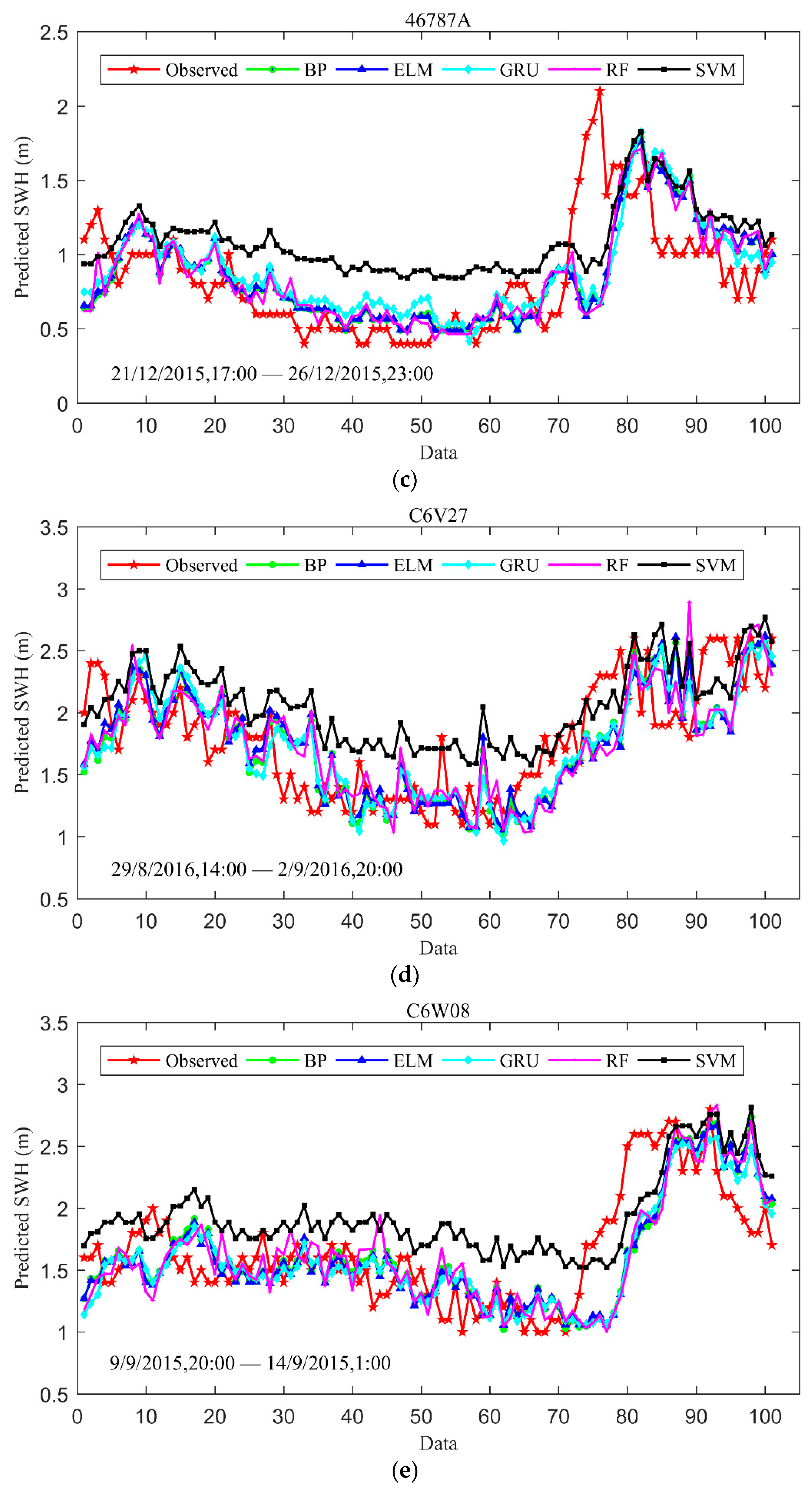
Figure 6 provides the comparison of the five different algorithms for the 6 h prediction. Although the forecasting accuracy decreased for all models, the deep learning method GRU yielded better prediction results and captured the trend of data relatively well. The superiority of using GRU in comparisons to the other four methods is because GRU is proficient at identifying previous essential information to estimate the current state. On the contrary, SVM, BP, RF and ELM belong to the shallow machine learning models. The insufficiency of shallow machine learning models has restricted their application in long-term time series prediction.

What cannot be ignored is that a great difference in SVM with respect to the others exists in the first panel of Figure 4 and Figure 6. There may be two possible reasons to explain this phenomenon. On the one hand, the parameter setting of SVM is considered according to the previous study and in balance with the computational time. Therefore, the parameter setting of SVM may not be optimal for every buoy station. On the other hand, the average SWH of 46714D is less than 1 m in the period selected, which is relatively small in comparison with others.

4.3. Long-Term Span SWH Prediction

The prediction results with lead times of 12 h and 24 h are listed in Table 5 and

Table 6. Error indices of predicted SWH with lead times of 24 h.

Station	Algorithm	RMSE	R	IA
46714D	GRU	0.479	0.735	0.808
	SVM	0.707	0.729	0.478
	BP	0.498	0.694	0.794
	ELM	0.950	0.475	0.613
	RF	0.509	0.682	0.803
46735A	GRU	0.612	0.619	0.726
	SVM	0.657	0.613	0.608
	BP	0.621	0.607	0.706
	ELM	0.738	0.445	0.636
	RF	0.624	0.597	0.717
46787A	GRU	0.413	0.546	0.641
	SVM	0.624	0.534	-0.1679
	BP	0.418	0.536	0.623
	ELM	0.892	0.172	0.297
	RF	0.426	0.514	0.627
C6V27	GRU	0.862	0.607	0.731
	SVM	0.918	0.603	0.632
	BP	0.866	0.601	0.725
	ELM	1.019	0.486	0.667
	RF	0.882	0.587	0.729
C6W08	GRU	0.805	0.629	0.691
	SVM	1.056	0.613	0.330
	BP	0.807	0.621	0.687
	ELM	1.330	0.259	0.452
	RF	0.822	0.600	0.690
NanJi	GRU	0.486	0.612	0.703
	SVM	0.593	0.569	0.484
	BP	0.496	0.587	0.702
	ELM	0.867	0.298	0.478
	RF	0.504	0.572	0.695

. The longer the prediction horizon is, the weaker the link in the data series is. Therefore, there is no doubt that RMSE increases, whereas R and IA decrease at the same time. However, the performance of GRU is still the best among these five algorithms and its prediction error was within an acceptable range with lead times up to 12 h and 24 h. It can be seen that the results obtained by ELM and SVM are invalid. At station 46714D, the RMSE obtained by GRU is only 0.371 for 12 hourly forecast, whereas the same indices of ELM and SVM are high, up to 0.840 and 0.663, which indicates that GRU has a stronger adaptability and reliability for long-term horizon prediction.

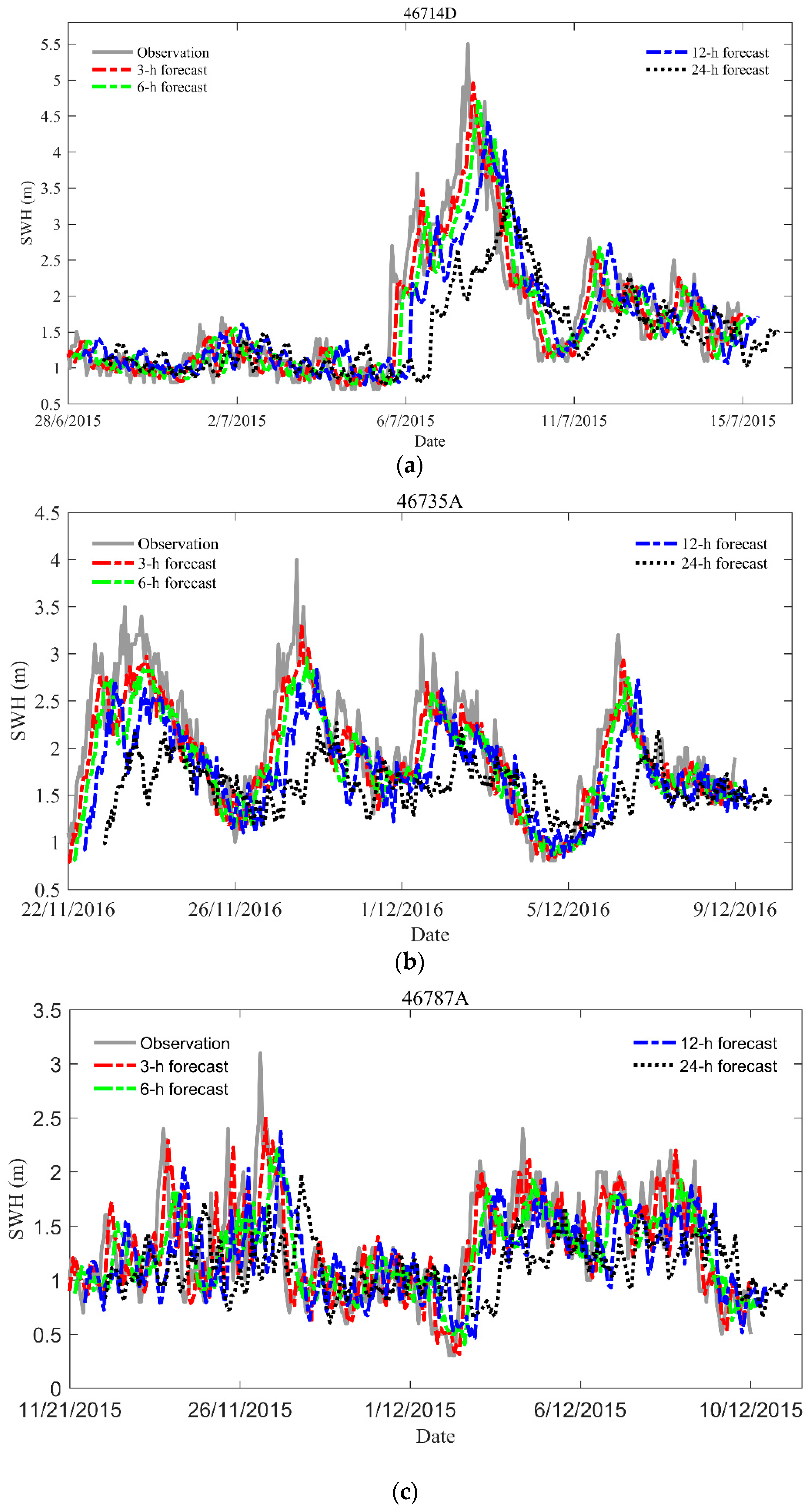
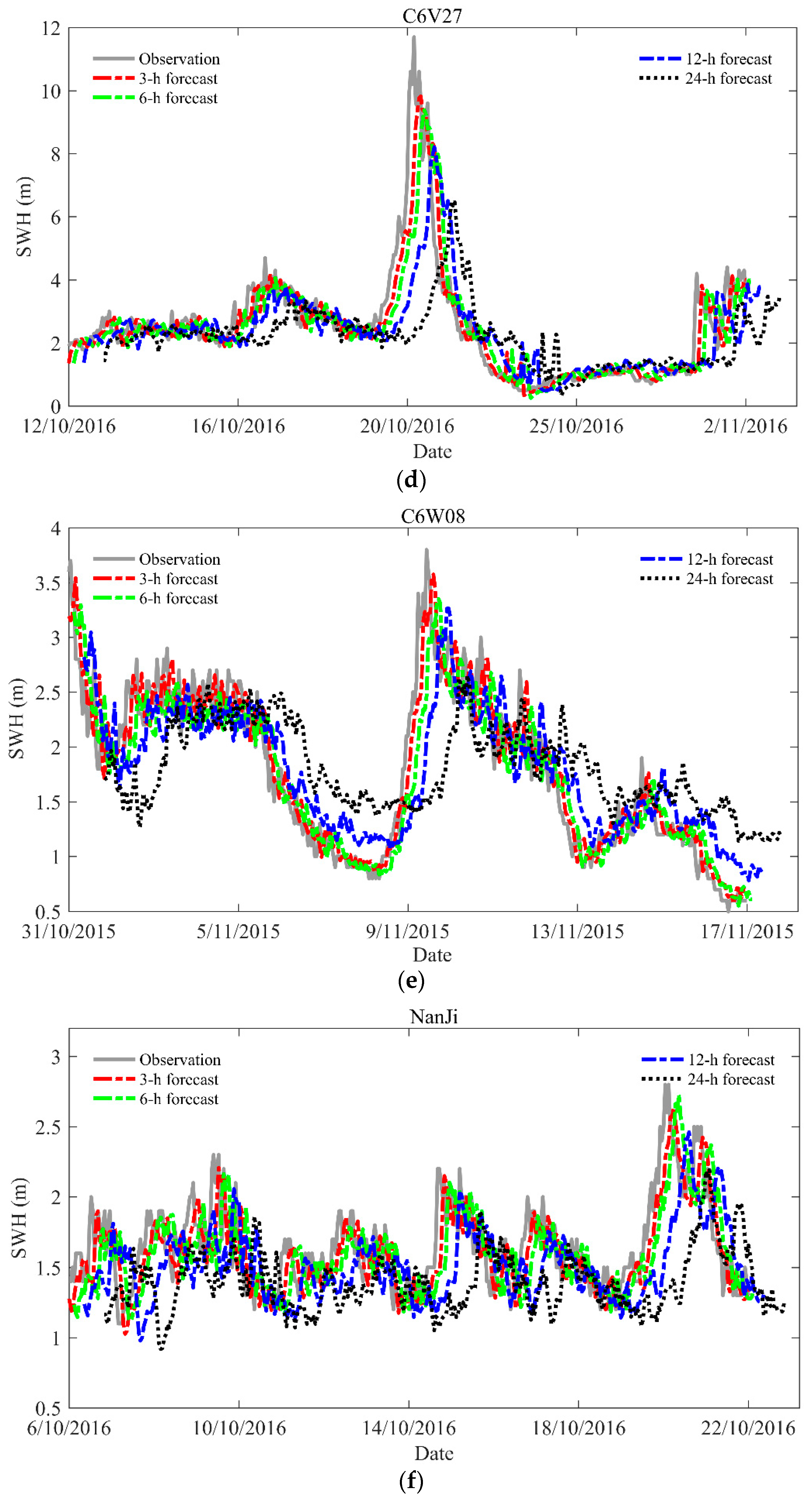
As shown in Figure 7, an obvious hysteresis in 24 h forecasting exists, but the general trends of the predicted SWH are consistent with the observed values. This may be because the dependence of the SWH on the previous wave characteristics decreases in a large forecasting time horizon.

In addition, it is somewhat disappointing to find that GRU underestimated the SWH for 12 h and 24 h forecasting, especially in extreme events at all stations. A possible explanation for these results might be that slight sea and moderate sea accounted for an overwhelming portion in the training process of GRU.

The peak SWH of 7.4 m observed on 8 August 2015 at 13:00 is predicted as 5.744, 5.699, 5.373, 3.961 m by GRU for lead times of 3 h, 6 h, 12 h, and 24 h at station 46714D. Station C6V27 suffered the Super Typhoon Haima on 20 October 2016, where the observed SWH was 11.7 m at 18:00. The prediction of peak made by GRU is 9.818, 9.383, 8.211, 6.464 m respectively for 3 h, 6 h, 12 h, and 24 h forecasts. The most likely cause of underestimation for larger wave heights is that usually the training datasets do not contain sufficient similar data for the peak wave height.

5. Conclusions

GRU is a novel deep learning method that is accomplished in retaining long-term information with high efficiency, which can provide fresh insight into the time series prediction. In this paper, the performance of GRU for SWH prediction with lead times of 3, 6, 12 and 24 h was investigated. To test the performance of GRU, current SWH and wind speed of the past 3 h collected from six buoy stations distributed at various sites in the Taiwan Strait and its adjacent waters were fed as inputs, and the error indicators RMSE, R, and IA were utilized to evaluate the accuracy.

Overall, it can be concluded that GRU has the ability to produce better forecasting values and capture the general data trend. By comparison, the predictions made by SVM and ELM are rather inaccurate and tend to have larger fluctuations. For BP and RF, the forecasting skill is slightly inferior to that of GRU. Because GRU has a strong edge in long-term time series prediction, the performance with lead times of 3 and 6 h are satisfactory and trustworthy. As forecasting time increased, the root mean square error increased and the coefficient of correlation decreased for all models. However, the error statistics of GRU are still within an acceptable range. Although GRU does not completely achieve success in predicting peak wave heights for extreme events, much of the underestimation can be attributed to the lack of sufficient similar large wave heights in the training database.

Benefitting from the recurrent structure and special gate mechanism, it is believed that GRU can provide SWH predictions with multistep lead times in a reliable and prompt way, which is favorable for coastal disaster risk reduction and mitigation management. As long as the forecasts exceed predefined threshold levels, hazard warnings with detailed scale will be issued immediately, which may give assistance to the authorities and decision-makers to create better preparedness for the sake of coastal residential communities and safe offshore operation. A further improvement on the SWH prediction accuracy is possible by provision of more input features such as wind direction and wave direction.

References

1. Zheng, C.-W.; Wu, G.-X.; Chen, X.; Wang, Q.; Gao, Z.-S.; Chen, Y.-G.; Luo, X. CMIP5-Based Wave Energy Projection: Case Studies of the South China Sea and the East China Sea. IEEE Access 2019, 7, 82753–82763. [Google Scholar] [CrossRef]
2. Zheng, C.W.; Li, C.Y. Variation of the wave energy and significant wave height in the China Sea and adjacent waters. Renew. Sust. Energ. Rev. 2015, 43, 381–387. [Google Scholar] [CrossRef]
3. Agrawal, J.D.; Deo, M.C. On-line wave prediction. Marine Struct. 2002, 15, 57–74. [Google Scholar] [CrossRef]
4. Guner, H.A.A.; Yuksel, Y.; Cevik, E.O. Estimation of wave parameters based on nearshore wind-wave correlations. Ocean Eng. 2013, 63, 52–62. [Google Scholar] [CrossRef]
5. Yoon, H.; Jun, S.-C.; Hyun, Y.; Bae, G.-O.; Lee, K.-K. A comparative study of artificial neural networks and support vector machines for predicting groundwater levels in a coastal aquifer. J. Hydrol. 2011, 396, 128–138. [Google Scholar] [CrossRef]
6. Zamani, A.; Solomatine, D.; Azimian, A.; Heemink, A. Learning from data for wind-wave forecasting. Ocean Eng. 2008, 35, 953–962. [Google Scholar] [CrossRef]
7. Malekmohamadi, I.; Bazargan-Lari, M.R.; Kerachian, R.; Nikoo, M.R.; Fallahnia, M. Evaluating the efficacy of SVMs, BNs, ANNs and ANFIS in wave height prediction. Ocean Eng. 2011, 38, 487–497. [Google Scholar] [CrossRef]
8. Altunkaynak, A.; Wang, K.-H. Estimation of significant wave height in shallow lakes using the expert system techniques. Expert Syst. Appl. 2012, 39, 2549–2559. [Google Scholar] [CrossRef]
9. Nitsure, S.P.; Londhe, S.N.; Khare, K.C. Wave forecasts using wind information and genetic programming. Ocean Eng. 2012, 54, 61–69. [Google Scholar] [CrossRef]
10. Prahlada, R.; Deka, P.C. Forecasting of Time Series Significant Wave Height Using Wavelet Decomposed Neural Network. In Proceedings of the International Conference on Water Resources, Coastal and Ocean Engineering (icwrcoe’15), Karnataka, India, 11–14 March 2015; Dwarakish, G.S., Ed.; Elsevier: Amsterdam, The Netherlands, 2015; Volume 4, pp. 540–547. [Google Scholar]
11. Cornejo-Bueno, L.; Nieto-Borge, J.C.; Garcia-Diaz, P.; Rodriguez, G.; Salcedo-Sanz, S. Significant wave height and energy flux prediction for marine energy applications: A grouping genetic algorithm—Extreme Learning Machine approach. Renew. Energy 2016, 97, 380–389. [Google Scholar] [CrossRef]
12. Nikoo, M.R.; Kerachian, R.; Alizadeh, M.R. A fuzzy KNN-based model for significant wave height prediction in large lakes. Oceanologia 2018, 60, 153–168. [Google Scholar] [CrossRef]
13. Wei, C.-C.; Hsieh, C.-J. Using Adjacent Buoy Information to Predict Wave Heights of Typhoons Offshore of Northeastern Taiwan. Water 2018, 10, 1800. [Google Scholar] [CrossRef] [Green Version]
14. Yang, S.; Xia, T.; Zhang, Z.; Zheng, C.; Li, X.; Li, H.; Xu, J. Prediction of Significant Wave Heights Based on CS-BP Model in the South China Sea. IEEE Access 2019, 7, 147490–147500. [Google Scholar] [CrossRef]
15. Zhang, X.; Dai, H. Significant Wave Height Prediction with the CRBM-DBN Model. J. Atmos. Oceanic Technol. 2019, 36, 333–351. [Google Scholar] [CrossRef]
16. Hochreiter, S.; Schmidhuber, J. Long short-term memory. Neural Comput. 1997, 9, 1735–1780. [Google Scholar] [CrossRef]
17. Son, G.; Choi, H.; Lee, J.-H.; Kang, P. Significant Wave Height Regression from a Raw Ocean Image with Convolutional LSTM and 3D Convolutional Networks. J. Korean Op. Res. Manag. Sci. Soc. 2020, 45, 11–24. [Google Scholar] [CrossRef]
18. Fan, S.; Xiao, N.; Dong, S. A novel model to predict significant wave height based on long short-term memory network. Ocean Eng. 2020, 205, 107298. [Google Scholar] [CrossRef]
19. Cho, K.; Merriënboer, B.V.; Gulcehre, C.; Bahdanau, D.; Bougares, F.; Schwenk, H.; Bengio, Y. Learning phrase representations using RNN encoder-decoder for statistical machine translation. In Proceedings of the EMNLP 2014 Conference on Empirical Methods in Natural Language Processing, Doha, Qatar, 25–29 October 2014; pp. 1724–1734. [Google Scholar] [CrossRef]
20. Zhao, R.; Wang, D.; Yan, R.; Mao, K.; Shen, F.; Wang, J. Machine Health Monitoring Using Local Feature-Based Gated Recurrent Unit Networks. IEEE Trans. Ind. Electron. 2018, 65, 1539–1548. [Google Scholar] [CrossRef]
21. Lee, K.; Kim, J.-K.; Kim, J.; Hur, K.; Kim, H. CNN and GRU Combination Scheme for Bearing Anomaly Detection in Rotating Machinery Health Monitoring. In Proceedings of the 2018 1st IEEE International Conference on Knowledge Innovation and Invention, Jeju Island, Korea, 23–27 July 2018; Meen, T.H., Ed.; Elsevier: Amsterdam, The Netherlands, 2018; pp. 102–105. [Google Scholar]
22. Liu, H.; Mi, X.; Li, Y.; Duan, Z.; Xu, Y. Smart wind speed deep learning based multi-step forecasting model using singular spectrum analysis, convolutional Gated Recurrent Unit network and Support Vector Regression. Renew. Energy 2019, 143, 842–854. [Google Scholar] [CrossRef]
23. Yu, C.; Li, Y.; Bao, Y.; Tang, H.; Zhai, G. A novel framework for wind speed prediction based on recurrent neural networks and support vector machine. Energy Convers. Manag. 2018, 178, 137–145. [Google Scholar] [CrossRef]
24. Peng, Z.; Peng, S.; Fu, L.; Lu, B.; Tang, J.; Wang, K.; Li, W. A novel deep learning ensemble model with data denoising for short-term wind speed forecasting. Energy Convers. Manag. 2020, 207, 112524. [Google Scholar] [CrossRef]
25. Zhang, D.; Kabuka, M.R. Combining weather condition data to predict traffic flow: A GRU-based deep learning approach. IET Intell. Transp. Syst. 2018, 12, 578–585. [Google Scholar] [CrossRef]
26. Dai, G.; Ma, C.; Xu, X. Short-Term Traffic Flow Prediction Method for Urban Road Sections Based on SpaceTime Analysis and GRU. IEEE Access 2019, 7, 143025–143035. [Google Scholar] [CrossRef]
27. Mahjoobi, J.; Etemad-Shahidi, A.; Kazeminezhad, M.H. Hindcasting of wave parameters using different soft computing methods. Appl. Ocean Res. 2008, 30, 28–36. [Google Scholar] [CrossRef]
Figure 1. Distribution of the six selected buoy stations (denoted by red dots) and water depth in the study area.
Water 13 00086 g001
Figure 2. Inner structure of the gated recurrent unit network (GRU).
Water 13 00086 g002
Figure 3. Scatter diagram for 3 hourly forecasting based on GRU at various stations: (a) station 46714D, (b) station 46735A, (c) station 46787A, (d) station C6V27, (e) station C6W08, (f) station NanJi.
Water 13 00086 g003aWater 13 00086 g003b
Figure 4. Comparison of five algorithms with lead times of 3 h at various stations: (a) station 46714D, (b) station 46735A, (c) station 46787A, (d) station C6V27, (e) station C6W08, (f) station NanJi.
Water 13 00086 g004aWater 13 00086 g004bWater 13 00086 g004c
Figure 5. Scatter diagram for 6 hourly forecasting based on GRU at various stations: (a) station 46714D, (b) station 46735A, (c) station 46787A, (d) station C6V27, (e) station C6W08, (f) station NanJi.
Water 13 00086 g005
Figure 6. Comparison of five algorithms with lead times of 6 h at various stations: (a) station 46714D, (b) station 46735A, (c) station 46787A, (d) station C6V27, (e) station C6W08, (f) station NanJi.
Water 13 00086 g006aWater 13 00086 g006bWater 13 00086 g006c
Figure 7. SWH prediction of four-time spans at six stations at various stations: (a) station 46714D, (b) station 46735A, (c) station 46787A, (d) station C6V27, (e) station C6W08, (f) station NanJi.
Water 13 00086 g007aWater 13 00086 g007b