Abstract
Flood data on a high temporal scale are required for the design of hydraulic structures, flood risk assessment, flood protection, and reservoir operations. Such flood data are typically generated using rainfall-runoff models through an accurate calibration process. The data also can be estimated using a simple relationship between the daily and the sub-daily flow records as an alternative to rainfall–runoff modelling. In this study, we propose an approach combining an artificial neural network (ANN) model for peak flow estimation and the steepness index unit volume flood hydrograph (SIUVFH) method for sub-daily flow disaggregation to generate hydrographs on an hourly time scale. The SIUVFH method is based on the strong relationship between the flood peak and the steepness index, which is defined as the difference between the daily flood peak and daily flow several days before the peak; it is also used for selecting a reference unit volume flood hydrograph to be scaled to obtain the sub-daily flood hydrograph. In this study, to improve the applicability of the SIUVFH method for locations with a weak relationship between the flood peak and steepness index, the ANN-based flood peak estimation was used as an additional indicator to determine a reference unit volume flood hydrograph. To apply the proposed method, ANN models for estimating the peak flows from the mean daily flows during peak and adjacent days were constructed for the studied dam sites. The optimal ANN structures were determined through Monte Carlo cross-validation. The results showed a good performance with statistical measurements of relative root mean square errors of 0.155–0.224, 0.208–0.301, and 0.244–0.382 for the training, validation, and testing datasets, respectively. An application of the combined use of the ANN-based peak estimation and the SIUVFH-based flow disaggregation revealed that the disaggregated hourly flows satisfactorily matched the observed flood hydrograph.
1. Introduction
Flood event data with high temporal resolutions are fundamental to the design of hydraulic structures, flood frequency analysis, flood risk assessment, and reservoir operations. However, observed flood data are often lacking over a short period of time (e.g., on an hourly basis) for a given site of interest. In this case, flood data are generally simulated via rainfall–runoff models [1,2,3,4,5] using relatively extensive records of rainfall data over short time intervals. The rainfall–runoff modeling requires in depth knowledge of the complex relationships between rainfall and runoff. For simplicity, the instantaneous peak flow (IPF) and flood hydrographs can be transformed from mean daily flow (MDF) data [6,7,8,9,10,11,12,13,14,15,16,17,18,19,20,21,22]. This transformation from temporally coarse to fine flow data has limitations in capturing the physical rainfall–runoff relationship and in applying to small catchments with flood durations of much less than one day such as flash floods, but the method can be useful for locations where the published flow records contain only daily flow data.
According to Chen et al. [6], typically there are three groups of method to estimate the IPF from the MDF. The first group of methods establishes a relationship between the peak ratio of IPF and its corresponding maximum mean daily flow (MMDF) and the basin characteristics [7,8,9,10,11]. The second group estimates IPF using the sequence of MDF data [12,13,14]. The third approach uses a flow disaggregation method [15], machine-learning models [16,17,18], and multiple regression models with the simulated MMDF [19,20,21,22].
In the first group of IPF estimation methods, Fuller [7], for the first time, related IPF and MMDF against the drainage area using data from 24 basins in the USA. Similarly, Ellis and Gray [8] developed several regression equations to estimate the peak ratio of IPF to MMDF using the drainage area in Canada. The Spanish Center for Public Works Studies and Experimentation (CEDEX) also provided 12 regional formulas to estimate the IPF by adjusting Fuller’s formula [9]. Other physiographic characteristics [10] or climatic variables [11] in addition to the drainage area have been used to estimate the IPF. Taguas et al. [10] developed a regional equation to estimate the IPF from the mean daily flow, drainage area, and mean annual rainfall for the southeast Mediterranean Basin of Spain, and demonstrated a significant increase in accuracy compared to the Fuller formula. Ding et al. [11] suggested statistical approaches including a simple regression model, multiple regression model, and temporal scaling method to transfer MDF quantiles into IPF quantiles with regard to the flood frequency analysis in northern Germany.
In the second group, Langbein [12] established a relationship between IPF and MMDF in terms of the ratio of preceding day MDF to MMDF and the ratio of succeeding day MDF to MMDF. Following Langbein’s method, several studies have been conducted to generalize the empirical formula for IPF estimation. Sangal [13] specifies IPF as a function of the mean daily flow data of three consecutive days, the peak day, and the previous and next peak days, under the assumption of a triangular hydrograph. Fill and Steiner [14] improved Sangal’s method by applying a correction factor. More recently, Chen et al. [6] developed a slope-based method to estimate the IPF from a sequence of MDFs, which reflects the rising and falling slopes of an MDF hydrograph. They evaluated the slope-based method together with the empirical formulas of Fuller, Sangal, and Fill and Steiner for 3800 flood events at 144 basins in Iowa, USA.
In the third group of studies, which is not related to the above two groups, Tan et al. [15] recommended the steepness index unit volume flood hydrograph (SIUVFH) approach to disaggregate daily flood flows into sub-daily flows. This method can reproduce the rising-limb of the flood hydrograph as well as the peak on a sub-daily scale. Machine-learning techniques have been used for IPF estimation. Dastorani et al. [16] and Shabani and Shabani [17] developed artificial neural network (ANN)-based methods for the estimation of the IPF from MDF data at different stations in Iran, and showed that ANN estimations had lower errors compared with the empirical formulas provided by Fuller, Sangal, and Fill and Steiner. Dastorani et al. [18] applied adaptive neuro-fuzzy inference system (ANFIS) and ANN for estimating the IPF from the MDF at eight stations in Iran. They demonstrated that the ANFIS-based method was more accurate than the ANN and existing empirical formulas. Jimeno-Saez et al. [19] also used machine-learning models of ANN and ANFIS to estimate the IPF from MMDF in 14 watersheds in Peninsular Spain, and compared the results of ANN and ANFIS with the best performing empirical formulas including those of Fuller, CEDEX, Sangal, and Fill and Steiner in each basin. For post-processing the daily flows simulated from the Hydrologiska Byråns Vattenbalansavdelning (HBV) hydrological model, Ding et al. [20] and Ding et al. [21] applied the multiple regression model of Ding et al. [11] to obtain IPF quantiles in the Aller-Leine river basin in northern Germany. Senent-Aparicio et al. [22] proposed a combined application of soil and water assessment tool (SWAT) simulation and machine-learning techniques for IPF prediction. They evaluated the performance of ANN, ANFIS, support vector machine, and extreme learning machine (ELM) methods to estimate the IPFs from MMDFs in the Ladra river basin, northwest Spain, and finally reproduced IPFs using an ELM model with simulated MMDFs from the SWAT model.
The rising curve of the hydrograph and flood peak are vital for the design of hydraulic structures and flood risk management, particularly for modeling the dynamics of water storage and release of dam operations. However, the aforementioned methods have sought only to estimate the instantaneous peak flow from daily flow, except for the SIUVFH approach [15], which is capable of capturing the sub-daily (e.g., hourly) flood hydrograph up to the flood peak. Tan et al. [15] stated that the steepness index approach takes advantage of the strong relationship between the standardized instantaneous flood peak and the standardized daily flood hydrograph rising-limb steepness index, which is defined as the standardized value of daily flow on the day of daily flood peak minus the daily flow ‘n’ days before the daily flood peak. However, in contrast, the steepness index method may have considerable uncertainty in IPF estimations when the relationships between the standardized instantaneous flood peak and the standardized daily flood hydrograph rising-limb steepness index are moderate and weak.
Therefore, the aim of this paper is to propose a coupling approach of the ANN-based IPF estimation method and the steepness-index-based flow disaggregation method for improving the rising-limb hydrograph on an hourly time scale. To this end, we first construct ANN models that can estimate hourly peak flows using mean daily flows for seven dam sites in South Korea. The optimal network structure for each site was determined based on the Monte-Carlo cross-validation procedure, and the performance was evaluated via comparison with several empirical formulas for IPF estimation. A case study is also illustrated to investigate the improvement of the previously developed SIUVFH-based flow disaggregation method using the ANN-based peak estimation as an indicator of the SIUVFH method.
2. Materials and Methods
2.1. Study Sites and Data
The seven sites, namely Seomjingang-dam, Soyangang-dam, Andong-dam, Yongdam-dam, Imha-dam, Chungju-dam, and Hwoingseong-dam, located in various parts of South Korea, were chosen for this study (Figure 1) as they have extensive flood data that are not likely to be influenced by upstream anthropogenic activities. The dams are located on the major rivers of Korea, with three of them located within the Han River basin, two located within the Nakdong River basins, one in the Geum River basin, and the remainder in the Seomjingang River basin. The dams were built to serve multiple purposes, such as flood control, water supply, and hydropower generation. Each reservoir of the studied dam sites set the restrict water level (RWL) for flood control. The excessive water volume above RWL should be released during the specific flood season from 21 June to 20 September.
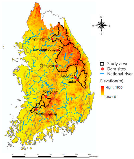
Figure 1.
Location of the study sites.
The sites are all characterized by monsoon climate, with two-thirds of the rainfall received in the summer. The flood event data sets were collected from the Water Resources Information System (WAMIS) available at the website, http://www.wamis.go.kr/. Table 1 provides attributes of the dam sites, including the site number, site name, drainage area, altitude, mean annual rainfall, mean annual runoff, collected record period, and number of floods used for the analysis. The drainage area varies from 209.0 km2 to 6648.0 km2, with altitudes from 147.5 m a.s.l. to 268.5 m a.s.l., and the number of events used for analysis from 44 to 51.

Table 1.
Hydrological and geomorphological characteristics of the study sites.
For each site, a set of flood events was selected from the observed hourly flows based on the peak-over-threshold concept. A threshold was set to obtain on average of about two flood events per year for each site. Each flood peak must exceed the threshold and be separated from the preceding or succeeding one by at least 5 days.
2.2. Empirical Methods for Estimating Instantaneous Peak Flow
Fuller [7] derived the relationship in Equation (1) in Table 2, using data from 24 river basins in the USA, to estimate the instantaneous peak flow (IPF), (m3/s) using the maximum mean daily flow (MMDF), (m3/s), and drainage basin area, A (km2). The regression coefficients can be modified for other regions by regressing the ratio of IPF over MMDF to the drainage area [6].
Table 2.
Empirical formulas for estimating the instantaneous peak flow (IPF) from the mean daily flows (MDFs).
Sangal [13] proposed an empirical formula, as shown in Equation (2), in which three consecutive days of mean daily flow data, including the MMDF of the peak day, the MDF of the previous day () and the MDF of the next day (), are used, assuming a triangular hydrograph.
Fill and Steiner [14] developed a formula, shown in Equation (3) similar to Sangal’s formula to estimate the instantaneous peak flow using the MMDF and the MDFs of the adjacent days. They additionally applied a correction factor k to obtain a better estimation of IPF. The correction factor was obtained from a linear regression between the hydrograph shape factor and k for 50 cases in Fill and Steiner’s study. As indicated by Chen et al. [6], Fill and Steiner’s formula allowed for a non-linear relationship between the IPF and MDFs because k is also a function of MDFs.
Chen et al. [6] recently proposed a slope-based method of estimating the IPF using a sequence of MDFs considering rising and falling slopes to describe the shape of MDF hydrographs. In the slope-based method, the IPF is expressed as in Equation (4) under the assumption that the intersection point of the extended rising and falling limbs of an MDF hydrograph is the associated IPF.
2.3. Steepness Index Unit Volume Flood Hydrograph Approach for Disaggregating Daily Flows
Tan et al. [15] developed a flow disaggregation method, termed the steepness index unit volume flood hydrograph (SIUVFH) approach, and they applied the method to the Latrobe River, Austria to generate hourly flood hydrographs using the daily flows modelled by the SIMHYD which is a simple lumped conceptual rainfall-runoff model, showing satisfactory results. In the SIUVFH method, daily flood flows are disaggregated into sub-daily flows under the prerequisites of a strong relationship between the standardized flood instantaneous flood peak (Equation (5)) and the standardized daily flood hydrograph rising-limb steepness index (Equation (6)).
where is the standardized instantaneous flood peak, is the instantaneous flood peak, and is the n + 1 -day flood volume from the preceding n day up to peak day as shown in Figure 2.
where is the standardized daily flood hydrograph rising limb steepness index, is the daily flood peak, and is the daily flow on preceding n days as shown in Figure 2.
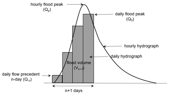
Figure 2.
Schematic of daily and hourly flood hydrographs, and the terms used in the steepness index unit volume hydrograph disaggregation approach.
To use the SIUVFH method, independent flood hydrographs are first selected and the hourly flows in each of them are then standardized and divided by . The standardized hourly hydrograph is named as an unit volume flood hydrograph (UVFH). Subsequently, the standardized instantaneous flood peak and the standardized daily flood hydrograph rising limb steepness index, are calculated using Equations (5) and (6) for each of the independent reference flood hydrographs. By gathering the pairs of and for all independent flood hydrographs, the relationships between both indices are plotted. If one would like to disaggregate a daily flood event into an hourly time scale, the n + 1 -day flood volume ( and the standardized daily flood hydrograph rising-limb steepness index () should be calculated. Here, two indices are accented by hats to differentiate the daily flood hydrograph to be disaggregated and the reference flood hydrographs. Finally, the hourly UVFH with closest to the is scaled by multiplied by to obtain the hourly flood hydrograph up to the flood peak.
2.4. Development of Artificial Neural Network (ANN)-Based Instantaneous Peak Flow (IPF) Estimation Method
An artificial neural network (ANN) is a type of machine-learning method that can adequately simulate non-linear complex systems without requiring a physical understanding of the underlying mathematical relationship between the input and output, and they have been widely used in hydrological fields [23,24,25,26]. The development of an ANN consists of partitioning the data, identifying important input variables, optimizing the network architecture and its parameters, and evaluating the model performance.
Many studies have used the cross-validation (CV) technique, such as holdout CV and k-fold CV, in which the learning data are divided into two subsets—training and test datasets. More recently, the learning data may be divided into three subsets of training, validation, and test datasets, where the validation set is used for early stopping. In the present study, the data were divided into three parts, including the training dataset to calibrate the weights of the network, the validation part for early stoppage of training progress to avoid overfitting, and the testing part for evaluating the performance of the optimized network.
Inappropriate division of the data into the training, validation, and test data sets will affect the selection of the optimal ANN structure and its prediction performance. To reduce the high variance of outputs, the Monte-Carlo cross-validation (MCCV) [27], denoted as a repeated random subsampling or random splitting, was used to compose the sub-data sets. The MCCV repeatedly performs cross-validation using randomly split datasets without replacement to obtain an ensemble of outputs and evaluate prediction errors. This approach is known to significantly reduce the variance of the model output [28]. Xu et al. [29], Barrow and Crone [30], and Lee et al. [31] successfully applied the MCCV method to hydrological prediction problems. However, the MCCV method has not been focused on flood peak estimation using ANN models with the input of the mean daily flows. Our study uses the MCCV method to generate an ensemble of flood peaks and to account for the uncertainty from various data subsampling and initial weight assignment.
We evaluated the model performance by increasing the training portion from 50% to 80% of the total data size with the increment of 10% (the rest are equally divided into validation and testing sizes). The results indicated that the different proportions had insignificant impacts on the training and validation stages, however, showed considerable impacts for testing stage. When focusing on the general performance for testing data set, the ratio of 60% of the data set for training, 20% for testing, and 20% for validation would be the optimal choice in this study. As indicated by Baxter et al. [32] and May et al. [33], these data splitting ratios have been known to be effective for ANN models. Therefore, the datasets available at each site were randomly split 100 times into three subsets of 60%, 20%, and 20% for training, validation, and testing, respectively. With additional random assignment of initial weights between nodes, we performed the MCCV a total of 10,000 times. That is, 100 by 100 runs with combinations of 100 times sub-data splitting and 100 sets of initial strengths between nodes for any one network structure.
Identifying the significant input variables that influence the output is important in developing an ANN model. Two types of ANN model were constructed for the IPF estimation. The first type of ANN model (ANN-1) had input variables of three consecutive days of mean daily flow including the peak daily flow, while the second (ANN-2) further used three consecutive days of areal rainfall amounts in addition to the input variables of ANN-1. Therefore, the number of input variables was set to 3, and it was increased to 6 in an attempt to investigate an improvement of the simulation accuracy by adding three consecutive daily rainfall data. The input and output data were normalized between −1.0 and 1.0 to account for the same scale as the limits of the activation function used in the hidden layer.
In this study, a multi-layer feed-forward neural network is used as an IPF simulation model, which had at least three layers: input, hidden, and output. The number of hidden layers was set to 1 for the simplicity of the network. The different number of hidden nodes was tested to find an optimal network architecture. The choice of the number of nodes in the hidden layer and, hence, the number of connection weights was important because too many weights can result in overtraining, while too few weights can undertrain the network. Empirical relationships between the number of connection weights and the number of training samples have been suggested in the literature [34]. For example, Rogers and Dowla [35] suggested that the number of weights should not exceed the number of samples. Masters [36] suggested that the number of training samples should be two times the number of weights, Weigend et al. [37] suggested 10 times. In our study, the training samples were not sufficient, so we followed the empirical rule of Rogers and Dowla [35]. Therefore, the number of weights would be appropriate below about 30–40, and, hence, the number of hidden nodes was desired to be about 5–10 when considering the number of inputs at 3–6. The desired number of hidden nodes can be reduced due to the addition of a bias term to the network. We initially set the maximum number of hidden nodes by 15 above the desired value, but finally chosen the optimal number to not exceed 10 by trial and error.
To reduce the variance of the training results affected by initial weights, an initial set of 100 weights between nodes was randomly assigned to the beginning of the training process. The backpropagation algorithm was used to update the weights of the network. A hyperbolic tangent sigmoid activation function was used in the hidden layer, and a linear activation function was used in the output layer.
The number of epochs for the training step highly depends on the ANN structure and complexity of the problem. In general, an ANN model improves with more epochs of training, but overfitting can occur when using too many epochs, which leads to reduction of the generalization ability of the model for unseen data. However, we have used an early stopping method for the validation set, therefore, the number of epochs is likely not the critical issue. We trained the network with sufficient epochs (5000) and terminated the training when the validation error was at its minimum. The network for the epoch with the minimum validation root mean squared error (RMSE) was selected for the evaluation process.
As the data splitting and initial weight assignment were repeated at random, different neural networks were created that gave different performances at the end of the training process. Therefore, we evaluated the network performance by averaging the errors in the output. This study adopted the relative root mean squared error (RRMSE), the coefficient of determination (R2), and the Nash–Sutcliffe efficiency (NSE) to evaluate the estimated results of the ANN models. The RRMSE, R2, and NSE values were calculated using Equations (7)–(9), respectively.
where is the number of samples, is the observed values, is the predicted values, is the average of the observed values, and is the average of the predicted values.
2.5. Combining ANN-Based Peak Flow Estimation and Steepness Index Unit Volume Flood Hydrograph (SIUVFH)-Based Sub-Daily Flow Disaggregation
The ANN model and the empirical formula specified in the sub-sections above can estimate the IPF using daily flow data, but the methods cannot reproduce flood hydrographs. The SIUVFH method is able to disaggregate a daily flood hydrograph by scaling an observed reference unit volume flood hydrograph pattern with a similar steepness index, however, the corresponding IPF significantly depends on which pattern is chosen. For locations with weak relationships between the standardized flood peak and the standardized steepness index, it is difficult to determine an appropriate unit volume flood hydrograph. To overcome the drawbacks of the above peak estimation method and flow disaggregation method, we combined the ANN model and the SIUVFH method to obtain hourly hydrographs. The SIUVFH method matches the event flood volume of interest with the volume of any one with a similar steepness index among the reference hydrographs. The combined approach suggested in this study additionally matches the peak flow (or the standardized flood peak ) of interest with the peak of the scaled reference hydrograph (or the reference unit volume flood hydrograph), in which is estimated by the ANN models. Figure 3 summarizes the combination of the ANN model and SIUVFH method.
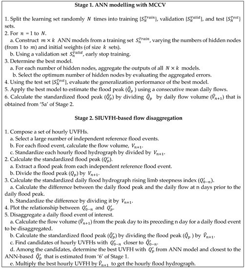
Figure 3.
Framework describing the combination of an artificial neural network (ANN) model and steepness index unit volume flood hydrograph (SIUVFH) method.
3. Results and Discussion
3.1. ANN-Based Estimation of Hourly Peak Flow
3.1.1. Optimal ANN Model
An ANN-1 model with input variables of three consecutive days of mean daily flows including the peak daily flow and an ANN-2 model with input variables of three consecutive days of areal rainfall amounts and mean daily flows were constructed. The RRMSE, NSE, and R2 between the observed and estimated hourly peaks for each site were calculated for the ANN-1 and ANN-2 models by changing the number of hidden neurons. Then, the optimal ANN structures were determined based on the minimum errors in the training and validation datasets.
Table 3 shows the values of RRMSE, NSE, and R2 of the optimal ANN-1 with different numbers of hidden neurons for the seven sites. The RMSE was normalized by dividing the value by the mean of the observed peak flows for comparing the model’s performance between sites. The ranges of the values of RRMSE, NSE, and R2 values for the training, validation, and testing datasets were 0.155–0.224, 0.858–0.956, and 0.867–0.956, 0.208–0.301, 0.731–0.863, and 0.789–0.924, and 0.244–0.382, 0.577–0.834, and 0.760–0.914, respectively. We concluded that the values of RRMSE, NSE, and R2 for the test dataset were acceptable with insignificant differences from the training and validation results.
Table 3.
Performance statistics of the optimal ANN-1.
Based on the minimum RRMSE and the maximum NSE and R2, the optimal ANN-2 was selected for each site. Table 4 presents the RRMSE, NSE, and R2 values of the optimal ANN-2 for each site. The optimal ANN-2 structures were different from that of ANN-1 due to the increase in the number of input variables. The RRMSE values were 0.110–0.196, 0.209–0.318, and 0.286–0.386 for the training, validation, and test datasets, respectively. The NSE values were 0.826–0.973, 0.636–0.849, and 0.495–0.761 for the training, validation, and test datasets, respectively. The R2 values were 0.916–0.978, 0.808–0.906, and 0.726–0.878 for the training, validation, and test datasets, respectively.
Table 4.
Performance statistics of the optimal ANN-2.
ANN-2 (Table 4) showed better performance than ANN-1 (Table 3) in terms of RRMSE, NSE, and R2 during training. However, during validation and testing, ANN-2 did not always show improved performance, even though a sequence of areal rainfall amounts were further considered as input variables. The accuracy of ANN-1 was better than that of ANN-2 during validation and testing at most sites. We finally selected ANN-1 with inputs of three consecutive daily mean flows to focus on the performance with respect to the unseen data and to match the input variables of other empirical IPF estimation methods for which the prediction performance was compared.
3.1.2. Comparison of ANN Model with Empirical Methods
To compare the results of the ANN-based peak estimation method with those of the Fuller, Sangal, Fill and Steiner, and slope-based methods, the values of the RMSE and percent bias (Pbias) were calculated for the seven sites studied. Table 5 and Table 6 show the values of the RMSE and Pbias for each site. The best results showing the lowest values of RMSE and Pbias for each site are highlighted in bold in the tables. The ANN model produced the most accurate results compared to the empirical methods. In general, the results obtained by Fuller’s method showed the worst performance in this study. Focusing on the Pbias, one can observe that all empirical methods generally showed negative Pbias, both Fuller’s and slope-based methods a high negative Pbias, leading to the underestimation of peak flow. This underestimation can cause a risky flood-protection design when it is used for flood frequency analysis. The ANN model showed a negligible positive Pbias; therefore, it can be considered the most superior method for peak estimation.
Table 5.
Values of the root mean squared error (RMSE, mm) of the estimated peak flows with different methods.
Table 6.
Values of percent bias (Pbias, %) of the estimated peak flows with different methods.
Figure 4 shows the scatter plots of the estimations from the ANN model and the four empirical formulas with the observed peak flows. The peak flow data used at seven sites were plotted together. In general, the estimated flood peaks using empirical formulas were more deviated from the observed peaks compared to the ANN model’s estimations. The regression line slope estimated by Sangal’s formulas was closer to 1 when compared with the others but showed wider dispersed points. The ANN results showed narrowly dispersed points along the regression line with the best performance in terms of the highest R2 of 0.966. The present study also confirms the high ability of the ANN model for the estimation of the instantaneous peak flow from the MDF data.
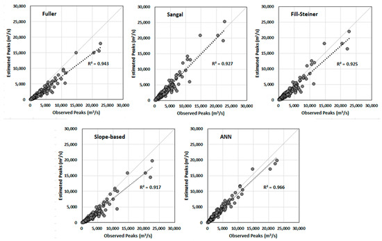
Figure 4.
Comparison of the estimated and observed peak flows.
3.2. Estimation of Hourly Flow Hydrographs
The proposed methodology combining an ANN model for peak flow estimation and the SIUVFH for flow disaggregation to generate a hydrograph on an hourly scale was applied to the Imha-dam site. As presented in Table 1, the 47 flood events for the Imha-dam sites were used as independent reference hydrographs. Each hydrograph was further standardized by dividing its hourly flows by the n+1 day flow volume to obtain the hourly unit volume flood hydrograph (UVFH). Then, the standardized hourly flood peak and the standardized daily flood hydrograph rising-limb steepness index were calculated using Equations (5) and (6) for all UVFHs. The relationships between and for different n-days are presented in Figure 5.
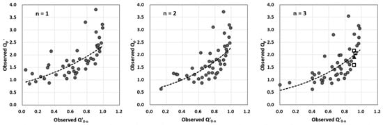
Figure 5.
Relationship between the standardized instantaneous flood peak and the standardized daily flood hydrograph rising-limb steepness index (unit: m3/s/ (86,400 m3)).
As can be seen from Figure 5, overall, the values of have an increasing trend as the values of increase, particularly showing a steeper increase and wider spread for a large range of . The relationship appears so weak that it dissatisfies the prerequisite of a strong relationship between and in the SIUVFH method. The values of significantly differ from each other regardless of the similar values of the steepness index , which makes it difficult to select one observed hourly UVFH. The disaggregated flows vary considerably depending on which UVFH is selected. This problem was overcome by using the ANN-based flood peak estimation as another indicator to choose the optimal UVFH in this study.
In Figure 5, the four points near = 0.9 for n = 3 were selected as an example to show how to disaggregate daily flows. The daily flood hydrograph corresponding to a point marked with a black triangle was disaggregated, and the hourly UVFHs corresponding to three points marked in rectangles were selected as the candidates of UVFHs to be scaled. Figure 6 shows the unit volume flood hydrograph and actual hydrographs corresponding to three candidates points.
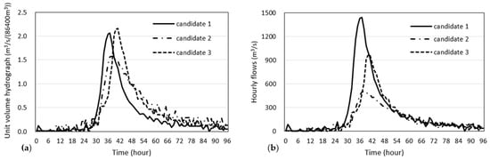
Figure 6.
Candidates of the observed hourly unit volume and actual hydrographs at the Imha-dam. (a) unit volume hydrograph; (b) actual hydrograph.
The 4-day flood volume and the steepness index of the daily flows to be disaggregated were calculated to be 354.8 86,400 m3 and 0.91, respectively. Using the ANN model for the Imha-dam site in Section 3.1, the flood peak was achieved to be 703.6 m3/s, which was further divided by to obtain the standardized flood peak of of 1.95. From the comparison of and the three candidates of UVFHs in Figure 6, we selected the UVFH of the candidate 1, which has = 2.03 similar to = 1.95. Finally, the selected UVHF was scaled by multiplying the flow volume to generate the hourly flood hydrograph as shown in Figure 7.
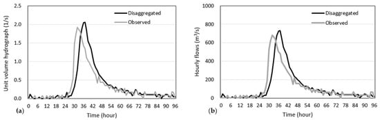
Figure 7.
Comparison of the observed and disaggregated flows at Imha-dam. (a) unit volume hydrographs (b) scaled hydrographs.
The figure indicates that the disaggregated daily flows satisfactorily match the observed hourly hydrograph. The difference between the observed and estimated flood peaks was about 50.0 m3/s, indicating overestimation by about 6.8%. From the figure, a roughly 4-h time shift between the observed and estimated flood peaks occurred. If there are more historical reference hydrographs that match both the flood peak and volume of the generated flood hydrograph, then an ensemble of flood hydrographs can be obtained. The ensemble can reduce the uncertainty of the disaggregated hydrograph, such as a difference in the time to the peak.
4. Conclusions
Obtaining flood data at high resolutions is of fundamental importance to design hydraulic structures for flood protection, operate reservoirs for flood management, and assess flood risks. For locations with a lack of instantaneous flow records or having only mean daily flow data, it is necessary to transform the temporally coarse flow data to the flood data on a finer time scale. This study constructed artificial neural network (ANN) models for estimating hourly peak flow for seven dam sites in South Korea, and improved the SIUVFH method for sub-daily flow disaggregation by combining the ANN-based peak estimation.
Two types of ANN model to estimate hourly peak flow from mean daily flows were constructed for each site: one had input variables of the maximum mean daily flow and the mean daily flows of the adjacent days, and the other had three consecutive days of daily rainfalls and mean daily flows. The number of hidden layers was set to 1, and its number of nodes was determined by trial and error. For each number of hidden nodes, a total of 10,000 different parameter sets with 100 times data sub-sampling and 100 sets of initial strengths between nodes were generated using the Monte-Carlo cross validation technique. The optimal number of hidden nodes per site was determined based on the statistical error evaluation. In terms of the RRMSE, NSE, and R2 between the estimated and observed hourly flood peaks, the ANN model with additional consideration of rainfall amounts during the peak day and adjacent days performed better for the training datasets. However, the simpler ANN model using only daily flows was adequate for the unseen data, showing a better general performance for the test datasets for most of the study sites. Therefore, the ANN model with inputs of three consecutive days of mean daily flows was finally chosen. The optimal ANN model resulted in RRMSE values of 0.244–0.382, NSE values of 0.577–0.834, and R2 values of 0.789–0.924 for the testing dataset. The optimal ANN models had lower errors of RRMSE and Pbias compared to the empirical formulas of Fuller, Sangal, Fill and Steiner, and slope-based methods, indicating the better performance in the flood peak estimation.
The SIUVFH method, a flow disaggregation approach, depends on a strong relationship between the flood peak and the steepness index (the daily peak flow minus the daily flow for n days before the peak day). The performance of the sub-daily flow generated by the SIUVFH method is governed by the selection of any reference sub-daily unit volume hydrograph with a similar steepness index to the daily flows of interest, which is scaled to match the event flood volume (scaled by multiplying the flow volume by the peak day from n-days before to obtain a sub-daily hydrograph). However, when the flood peak has a weak relationship with the steepness index, it is difficult to select an appropriate unit volume hydrograph. To overcome this circumstance, we improved the SIUVFH method to better represent the rising shape of the hydrograph up to the flood peak by using the hourly peak value estimated from the pre-developed ANN model. That is, the peak estimation was further used as an indicator in addition to the steepness index to select an optimal reference unit volume hydrograph. The suitability of the proposed disaggregation approach combining the ANN model and SIUVFH method was demonstrated through application to a dam site. Visual inspection indicated that the magnitude and pattern of the disaggregated flows satisfactorily reproduce the actual observed hydrograph. We concluded that the linkage of the ANN model and a flow disaggregation method strengthened the potential to estimate a better flood hydrograph using the daily flow data.
The proposed combination of the ANN and SIUVFH methods was based on the mean daily flow data, which is useful in the case of published flow records that contain such data. However, since flood data as an input variable are gathered on a daily basis, cases where the flood duration is less than one day, such as for a flash flood, may be inappropriate for small catchments. This drawback can be overcome if sub-hourly flow data (e.g., in minutes) exist. The proposed approach can be extended to an hourly flow disaggregation problem by establishing the relationship between a minute-based flood peak as an output variable and a consecutive hourly based flow as the input variable. Given that better accuracy in predicting flood peaks yields a better performance of the proposed flow disaggregation, advanced machine-learning techniques will be essential in the future to increase the accuracy of flood peak estimation.
Author Contributions
Formal analysis, J.E.L.; Investigation, J.L., J.E.L. and N.W.K.; Methodology, J.L.; Supervision, N.W.K.; Validation, J.L. and N.W.K.; Writing—original draft, J.L., J.E.L. and N.W.K.; Writing—review & editing, J.E.L. All authors read and agreed to the published version of the manuscript.
Funding
This research was funded by the Korea Institute of Civil Engineering and Building Technology (grant number 20200027-001) and the APC was funded by the Korea Institute of Civil Engineering and Building Technology.
Institutional Review Board Statement
Not applicable.
Informed Consent Statement
Not applicable.
Data Availability Statement
The data presented in this study are available on request from the corresponding author.
Acknowledgments
This research was supported by a grant from a Strategic Research Project (Developing technology for water scarcity risk assessment and securing water resources of small and medium-sized catchments against abnormal climate and extreme drought) funded by the Korea Institute of Civil Engineering and Building Technology.
Conflicts of Interest
The authors declare no conflict of interest.
References
- Camici, S.; Ciabatta, L.; Massari, C.; Brocca, L. How reliable are satellite precipitation estimates for driving hydrological models: A verification study over the Mediterranean area. J. Hydrol. 2018, 563, 950–961. [Google Scholar] [CrossRef]
- Cislaghi, A.; Masseroni, D.; Massari, C.; Camici, S.; Brocca, L. Combining a rainfall–runoff model and a regionalization approach for flood and water resource assessment in the western Po Valley, Italy. Hydrol. Sci. J. 2020, 65, 348–370. [Google Scholar] [CrossRef]
- Masseroni, D.; Cislaghi, A.; Camici, S.; Massari, C.; Brocca, L. A reliable rainfall–runoff model for flood forecasting: Review and application to a semi-urbanized watershed at high flood risk in Italy. Hydrol. Res. 2017, 48, 726–740. [Google Scholar] [CrossRef]
- Masseroni, D.; Cislaghi, A. Green roof benefits for reducing flood risk at the catchment scale. Environ. Earth Sci. 2016, 75, 579. [Google Scholar] [CrossRef]
- Hromadka, T.V. Rainfall-runoff models: A review. Environ. Softw. 1990, 5, 82–103. [Google Scholar] [CrossRef]
- Chen, B.; Krajewski, W.F.; Liu, F.; Fang, W.; Xu, Z. Estimating instantaneous peak flow from mean daily flow. Hydrol. Res. 2017, 48, 1474–1488. [Google Scholar] [CrossRef]
- Fuller, W.E. Flood flows. Trans. Am. Soc. Civ. Eng. 1914, 77, 564–617. [Google Scholar]
- Ellis, W.; Gray, M. Interrelationships between the peak instantaneous and average daily discharges of small prairie streams. Can. Agric. Eng. 1966, 8, 1–39. [Google Scholar]
- Centre for Public Works Studies and Experimentation (CEDEX). Mapa de Caudales Máximos: Memoria Técnica; CEDEX: Madrid, Spain, 2011. (In Spanish) [Google Scholar]
- Taguas, E.V.; Ayuso, J.L.; Pena, A.; Yuan, Y.; Sanchez, M.C.; Giraldez, J.V.; Prez, R. Testing the relationship between instantaneous peak flow and mean daily flow in a Mediterranean Area Southeast Spain. Catena 2008, 75, 129–137. [Google Scholar] [CrossRef]
- Ding, J.; Haberlandt, U.; Dietrich, J. Estimation of the instantaneous peak flow from maximum daily flow: A comparison of three methods. Hydrol. Res. 2015, 46, 671–688. [Google Scholar] [CrossRef][Green Version]
- Langbein, W.B. Peak discharge from daily records. Water Resour. Bull. 1944, 10, 145. [Google Scholar]
- Sangal, B.P. Practical method of estimating peak flow. J. Hydraul. Eng. 1983, 109, 549–563. [Google Scholar] [CrossRef]
- Fill, H.D.; Steiner, A.A. Estimating instantaneous peak flow from mean daily flow data. J. Hydrol. Eng. 2003, 8, 365–369. [Google Scholar] [CrossRef]
- Tan, K.-S.; Chiew, F.H.S.; Grayson, R.B. A steepness index unit volume flood hydrograph approach for sub-daily flow disaggregation. Hydrol. Process. 2007, 21, 2807–2816. [Google Scholar] [CrossRef]
- Dastorani, M.T.; Salimi, J.; Talebi, A.; Abghari, H. River instantaneous peak flow estimation using mean daily flow data. In Proceedings of the 9th International Conference on Hydroinformatics (HIC 2010), Tianjin, China, 7 September–15 October 2010; pp. 862–866. [Google Scholar]
- Shabani, M.; Shabani, N. Application of artificial neural networks in instantaneous peak flow estimation for Kharestan Watershed, Iran. J. Resour. Ecol. 2012, 3, 379–383. [Google Scholar]
- Dastorani, M.T.; Koochi, J.S.; Darani, H.S.; Talebi, A.; Rahimian, M.H. River instantaneous peak flow estimation using daily flow data and machine-learning-based models. J. Hydroinform. 2013, 15, 1089–1098. [Google Scholar] [CrossRef]
- Jimeno-Saez, P.; Senent-Aparicio, J.; Perez-Sanchez, J.; Pulido-Velazquez, D.; Cecilia, J.M. Estimation of instantaneous peak flow using machine-learning models and empirical formula in Peninsular Spain. Water 2017, 9, 347. [Google Scholar] [CrossRef]
- Ding, J.; Wallner, M.; Müller, H.; Haberlandt, U. Estimation of instantaneous peak flows from maximum mean daily flows using the HBV hydrological model. Hydrol. Process. 2016, 30, 1431–1448. [Google Scholar] [CrossRef]
- Ding, J.; Haberlandt, U. Estimation of instantaneous peak flow from maximum daily flow by regionalization of catchment model parameters. Hydrol. Process. 2017, 31, 612–626. [Google Scholar] [CrossRef]
- Senent-Aparicio, J.; Jimeno-Saez, P.; Bueno-Crespo, A.; Perez-Sanchez, J.; Pulido-Velazquez, D. Coupling machine-learning techniques with SWAT model for instantaneous peak flow prediction. Biosyst. Eng. 2019, 177, 67–77. [Google Scholar] [CrossRef]
- Chang, F.J.; Guo, S. Advances in hydrologic forecasts and water resources management. Water 2020, 12, 1819. [Google Scholar] [CrossRef]
- Chang, F.J.; Hsu, K.; Chang, L.C. (Eds.) Flood Forecasting Using Machine Learning Methods; MDPI: Basel, Switzerland, 2019. [Google Scholar] [CrossRef]
- Kao, I.-F.; Zhou, Y.; Chang, L.C.; Chang, F.-J. Exploring a Long Short-Term Memory based Encoder-Decoder framework for multi-step-ahead flood forecasting. J. Hydrol. 2020, 583, 124631. [Google Scholar] [CrossRef]
- Zhou, Y.; Guo, S.; Chang, F.-J. Explore an evolutionary recurrent ANFIS for modelling multi-step-ahead flood forecasts. J. Hydrol. 2019, 570, 343–355. [Google Scholar] [CrossRef]
- Picard, R.R.; Cook, R.D. Cross-validation of regression models. J. Am. Stat. Assoc. 1984, 79, 575–583. [Google Scholar] [CrossRef]
- Shao, J. Linear model selection by cross-validation. J. Am. Stat. Assoc. 1993, 88, 486–494. [Google Scholar] [CrossRef]
- Xu, Q.S.; Liang, Y.Z.; Du, Y.P. Monte Carlo cross-validation for selecting a model and estimating the prediction error in multivariate calibration. J. Chemom. 2004, 18, 112–120. [Google Scholar] [CrossRef]
- Barrow, D.K.; Crone, S.F. Cross-validation aggregation for combining autoregressive neural network forecasts. Int. J. Forecast. 2016, 32, 1120–1137. [Google Scholar] [CrossRef]
- Lee, J.; Kim, C.G.; Lee, J.E.; Kim, N.W.; Kim, H.J. Medium-Term Rainfall Forecasts Using Artificial Neural Networks with Monte-Carlo Cross-Validation and Aggregation for the Han River Basin, Korea. Water 2020, 12, 1743. [Google Scholar] [CrossRef]
- Baxter, C.W.; Stanley, S.J.; Zhang, Q.; Smith, D.W. Developing artificial neural network models of water treatment processes: A guide for utilities. J. Environ. Eng. Sci. 2002, 1, 201–211. [Google Scholar] [CrossRef]
- May, R.J.; Maier, H.R.; Dandy, G.G. Data splitting for artificial neural networks using SOM-based stratified sampling. Neural Netw. 2010, 23, 283–294. [Google Scholar] [CrossRef]
- Maier, H.R.; Dandy, G.C. Neural networks for the prediction and forecasting of water resources variables: A review of modelling issues and applications. Environ. Model. Softw. 2000, 15, 101–124. [Google Scholar] [CrossRef]
- Rogers, L.L.; Dowla, F.U. Optimization of groundwater remediation using artificial neural networks with parallel solute transport modeling. Water Resour. Res. 1994, 30, 457–481. [Google Scholar] [CrossRef]
- Masters, T. Practical Neural Network Recipes in C++; Academic Press: San Diego, CA, USA, 1993. [Google Scholar]
- Weigend, A.S.; Rumelhart, D.E.; Huberman, B.A. Predicting the future: A connectionist approach. Int. J. Neural Syst. 1990, 1, 193–209. [Google Scholar] [CrossRef]


Publisher’s Note: MDPI stays neutral with regard to jurisdictional claims in published maps and institutional affiliations. |
© 2020 by the authors. Licensee MDPI, Basel, Switzerland. This article is an open access article distributed under the terms and conditions of the Creative Commons Attribution (CC BY) license (http://creativecommons.org/licenses/by/4.0/).