Groundwater Response of Loess Tableland in Northwest China under Irrigation Conditions

Abstract

Water induced loess landslides are closely related to the rise of the groundwater level. Therefore, research on the response of the groundwater level to irrigation water holds promise for revealing the mechanism of water-induced loess landslide. Taking Heitai, Gansu Province, as the research area, a coupling model o unsaturated-saturated water movement is established using the HYDRUS-MODFLOW software. The parameters of the model are calibrated and verified by the Bayesian parameter inversion method combined with field observations of the groundwater level. Finally, the change in the groundwater level under different irrigation amounts is predicted using the optimized model. It is found that a reasonable reduction of the irrigation amount can effectively slow the rise of the groundwater level. This research provides a scientific reference for the development of reasonable irrigation measures.

1. Introduction

Loess is a special deposit that is formed in the Quaternary with weak cementation and is widely distributed throughout the world. In recent years, loess landslides triggered by agricultural irrigation have attracted the attention of engineering geologists [1,2,3]. The rise of the groundwater level caused by agricultural irrigation is the essential cause of the development of landslides in the irrigation area [4,5,6]. Therefore, research on the response of groundwater systems under irrigation conditions is the basis for revealing the mechanism of landslides.

Most traditional groundwater models split the complex transformation relationship between soil water and groundwater, resulting in a systematic deviation of the simulation results. To better simulate the flow and storage process of water in a basin, soil water and groundwater should be considered simultaneously to build a comprehensive hydrological model [7,8,9,10,11,12]. At present, many unsaturated-saturated coupling models have been developed, but they are quite different in terms of grid division, coupling mode, and other aspects [13,14,15]. In the coupling of the hydrological model SWAT and the groundwater model MODFLOW, the flow flux between the layers of the unsaturated zone is calculated by the water balance equation [16,17]. SWAT comprehensively considers crop growth, agricultural water management measures, farmland irrigation, and other aspects, but the interaction between the unsaturated system and groundwater system is poor [18]. The MODFLOW-SVAT coupling model couples the soil water movement model SVAT and the groundwater movement model MODFLOW [19]. The unsaturated zone flow movement is calculated by the water balance model. M. Kuznetsov et al. proposed a method to solve three-dimensional variable saturation flow by using the quasi three-dimensional Richards equation and the finite difference scheme. They established the saturated-unsaturated quasi-3D model on this basis [20]. The UZF1-MODFLOW model simplifies the one-dimensional Richards equation as a motion wave to describe the movement process of unsaturated soil flow [21,22]. The dynamic interface between the saturated zone and the unsaturated zone is weakened to avoid the vertical dispersion problem in the calculation of unsaturated soil water. However, the UZF1-MODFLOW model can only be applied to uniform media. MODFLOW-VSF is a three-dimensional saturated-unsaturated flow coupling model that uses the Richards equation to accurately describe the flow movement in the unsaturated zone, which can ensure high simulation accuracy [23]. However, solving the three-dimensional Richards equation also greatly increases the calculation cost, which also limits the applicability of the coupling model in regional simulations. MODFLOW-HYDRUS has a good balance between simulation accuracy and calculation cost for large scale simulations [24]. In terms of the scope of application, for groundwater flow at a large scale, the simulation accuracy of the HYDRUS model is significantly higher than that of UZF1 and its simulation efficiency is higher than that of VSF.

Determining the numerical model parameters is the premise of model applicability [25,26]. At present, the methods to obtain the parameters of water movement can be roughly divided into experimental methods and inversion methods [27,28]. Due to the scale effect, results obtained in the laboratory are usually difficult to apply to the simulation of the actual site size [29]. Although the field test method is more representative than the indoor test method, it usually consumes more resources and time, which also limits the application of the field method [30]. In the case of limited access to hydraulic parameters through experimental methods, people often use indirect methods to obtain soil hydraulic parameters based on easily accessible observation values [31,32]. The optimization method and random method are widely utilized in parameter inversion. The optimization method determines the optimal parameters of the model that can minimize the objective function [33,34]. The parameters obtained by optimization methods may be local optimal solutions, lacking uncertainty analysis of parameters. Although some optimization methods have the above disadvantages, they have little computation cost and can provide a reference for other methods. To quantify the parameter uncertainty more accurately, we can use the random parameter estimation method [35].

The main contents of this paper are:

• Taking Heitai, Gansu Province, as the research area, an unsaturated-saturated coupling flow model was established using the HYDRUS-MODFLOW software combined with rainfall, irrigation, and evaporation data;
• Combining groundwater level data monitored in the field with the Bayesian-MCMC random parameter inversion method, the optimization model is obtained by parameter calibration and model verification;
• Using the optimized model to predict the change of the trend of the groundwater flow field under different irrigation conditions and exploring effective measures to slow the rise of the groundwater level.

2. Materials and Methods

2.1. Basic Theory of Numerical Simulation

2.1.1. Unsaturated Transport Control Equation

The Richards equation can describe the law of soil water movement, which is as follows:

$$\frac{\partial \mathsf{\theta }\left(\mathrm{h}\right)}{\partial \mathrm{t}}=\frac{\partial }{\partial \mathrm{z}}[\mathrm{K}(\mathrm{h})\frac{\partial \mathrm{h}}{\partial \mathrm{z}}-\mathrm{K}(\mathrm{h})]-\mathrm{S}(\mathrm{h}),$$

(1)

where θ is the volume water content (${\mathrm{L}}^3{\mathrm{L}}^{-3}$); h is the pressure head (L); K(h)is the unsaturated hydraulic conductivity (L${\mathrm{T}}^{-1}$); Z is the vertical depth (L); t is the time (T); S(h) is the source and sink term (${\mathrm{L}}^3{\mathrm{L}}^{-3}{\mathrm{T}}^{-1}$). To solve this equation, we choose the Van Genuchten model to describe the relationship between the water content and pressure head and the Mualem model to describe the relationship between the unsaturated hydraulic conductivity and pressure head. The specific form of van Genuchten-Mualem (VGM) model is as follows:

$$\mathsf{\theta }\left(\mathrm{h}\right)=\{\begin{array}{cc}{\mathsf{\theta }}_{\mathrm{r}}+\frac{{\mathsf{\theta }}_{\mathrm{s}}-{\mathsf{\theta }}_{\mathrm{r}}}{{\left(1+{\left|\mathsf{\alpha }\mathrm{h}\right|}^{\mathrm{n}}\right)}^{\mathrm{m}}},& \mathrm{h}<0\\ {\mathsf{\theta }}_{\mathrm{s}},& \mathrm{h}\ge 0\end{array},$$

(2)

$$\mathrm{K}(\mathrm{h})=\{\begin{array}{cc}{\mathrm{K}}_{\mathrm{s}}{\mathrm{S}}_{\mathrm{e}}{}^{1/2}{[1-{\left(1-{\mathrm{S}}_{\mathrm{e}}{}^{1/\mathrm{m}}\right)}^{\mathrm{m}}]}^2,& \mathrm{h}<0\\ {\mathrm{K}}_{\mathrm{s}},& \mathrm{h}\ge 0\end{array},$$

(3)

where ${\mathrm{S}}_{\mathrm{e}}=\frac{\mathsf{\theta }-{\mathsf{\theta }}_{\mathrm{r}}}{{\mathsf{\theta }}_{\mathrm{s}}-{\mathsf{\theta }}_{\mathrm{r}}}$ is the effective saturation; ${\mathsf{\theta }}_{\mathrm{s}}$ is the saturated water content; ${\mathsf{\theta }}_{\mathrm{r}}$ is the residual water content; α is the parameter related to the average particle size; and n is the parameter related to the particle size uniformity, m = 1–1/n.

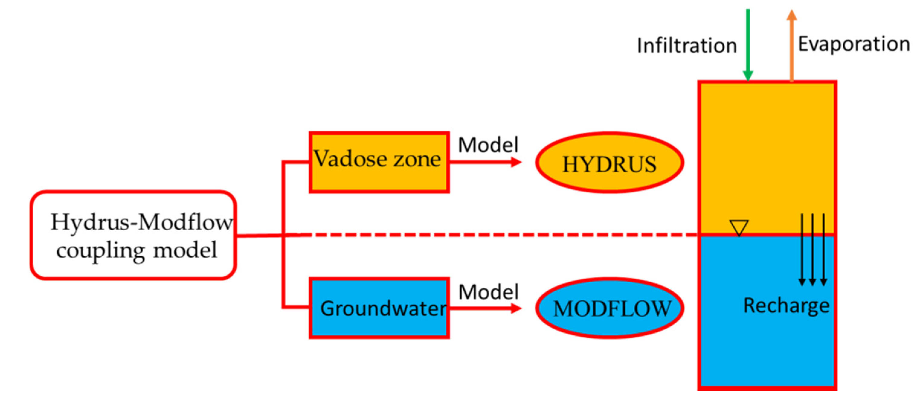
2.1.2. Basic Theory of the HYDRUS-MODFLOW Model

MODFLOW software has powerful functions to solve various problems related to groundwater flow. The theoretical basis of the numerical simulation of groundwater flow is the three-dimensional movement equation of groundwater in porous media. The equation of motion is derived according to the law of conservation of mass. The three-dimensional partial differential equation of groundwater unsteady flow is as follows:

$$\frac{\partial }{\partial x}\left(K_{xx}\frac{\partial H}{\partial x}\right)+\frac{\partial }{\partial y}\left(K_{yy}\frac{\partial H}{\partial y}\right)+\frac{\partial }{\partial z}\left(K_{zz}\frac{\partial H}{\partial z}\right)+W=S_s\frac{\partial H}{\partial t},$$

(4)

where $K_{xx}$, $K_{yy}$ and $K_{zz}$ are the components of the hydraulic conductivity in the x, y, and z coordinate directions under the assumption that the main axis direction of the permeability coefficient is consistent with the coordinate axis direction (L${\mathrm{T}}^{-1}$); H is the groundwater level (L); x, y, and z are the spatial coordinates; W is the source sink term (${\mathrm{L}}^3{\mathrm{L}}^{-3}{\mathrm{T}}^{-1}$); $S_s$ is the water storage coefficient, which is dimensionless; and t is the time (T). The most remarkable feature of MODFLOW is its modular structure. MODFLOW first introduced the concept of the stress period, which can be divided into a series of stress periods during the whole simulation period. Each stress period can be further divided into several time steps. MODFLOW uses the centre difference in space and the backward difference in time to obtain a discrete equation [36].

In the coupled HYDRUS-MODFLOW model, two independent control equations are applied to simulate the flow in the saturated zone and the unsaturated zone. The HYDRUS model focuses on the simulation of soil water in the unsaturated zone, and the MODFLOW model mainly simulates the movement process of groundwater in the saturated zone. By embedding the subroutine package HYDRUS into the main program MODFLOW of the groundwater model and taking the water surface as the interface, these equations can effectively simulate the water exchange process between saturated and unsaturated zones. Figure 1 shows a schematic diagram of the HYDRUS-MODFLOW coupling model:

The effect of the HYDRUS-MODFLOW coupling model depends to a great extent on how the two models interact in time and space. The simulation area in MODFLOW is divided into several zones, and the average groundwater depth of all the units in a zone determines the pressure head at the bottom boundary of the HYDRUS profile. The calculation method is as follows:

HB = (ZSURF − DEPTH) − Zl,

(5)

where HB is the bottom pressure head of the soil profile (L); ZSURF is the surface elevation (L); DEPTH is the buried depth of the groundwater level (L); and Z1 is the coordinate of the bottom of the soil profile (L). The time step of the HYDRUS model is independent and less than that of MODFLOW. The HYDRUS-MODFLOW coupling model simulates the flow in saturated and unsaturated zones through the discrete interaction of space and time and through the iterative cycle of a stress period.

2.1.3. Bayesian-MCMC Parameter Inversion Method

The Bayesian method is a recently popular random method, and it is based on the Bayesian principle:

$$\mathrm{P}\left(\mathrm{m}\right|\mathrm{d})\propto \mathrm{P}(\mathrm{m}\left)\mathrm{P}\right(\mathrm{d}\left|\mathrm{m}\right),$$

(6)

where P(m) is the prior distribution of model parameters, which is our understanding of the model parameters before obtaining the observation value d; P (m|d) is the posterior distribution of model parameters, which is our updated and more accurate understanding of the model parameters after obtaining the observation value d; and P(d|m) is the likelihood ratio, which is a measure of the proximity between the model output F (m) and the observation value d. Because most groundwater models are nonlinear, we cannot obtain an analytical expression of the posterior distribution of the model parameters. The Markov chain Monte Carlo (MCMC) method can be used to sample the posterior distribution of the parameters and estimate the posterior distribution of the model parameters. Vrugt and his partners further proposed the DREAM algorithm, which is a multi-chain MCMC algorithm [37].

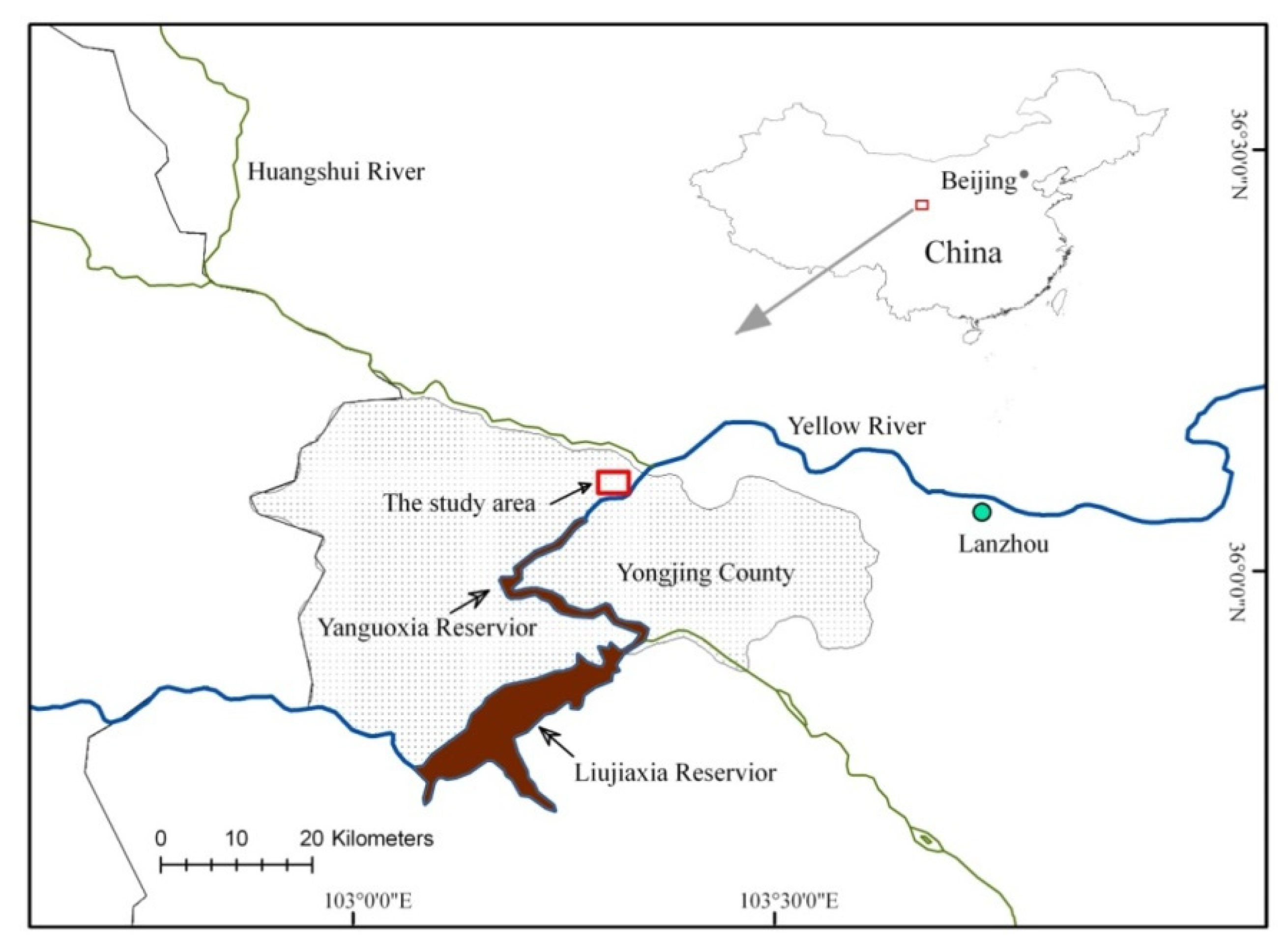
2.2. Geological Environment Conditions of Heitai, Gansu Province

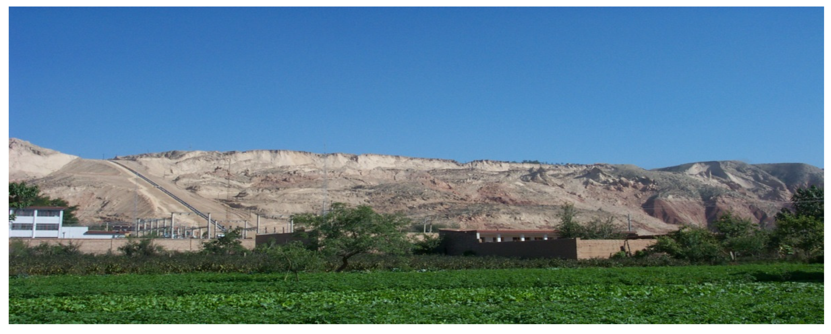
2.2.1. Topographic Features

Heitai is located on the north bank of the Yellow River at the intersection of the Yellow River and the Huangshui River (Figure 2). The total area of the tableland is approximately 10.8 km². The tableland surface is flat and broad, and the slope of the tableland surface is less than 5%. Because of the influence of landslide and collapse, there are many mounds under the tableland, and the ground is uneven (Figure 3).

2.2.2. Stratigraphic Structure and Aquifer Characteristics

The stratigraphic structure of the study area from top to bottom is: Loess, silty clay, pebble layer, and siltstone. According to the characteristics of the lithologic combination of the tableland in the area, the loose and porous loess easily seeps in the vertical direction, the dense silty clay layer is relatively water-proof, the gravel layer has excellent infiltration runoff conditions, and the sand mudstone is relatively water-proof. Therefore, the Heitai tableland is composed of three water-bearing rock groups: loess, sand gravel, and bedrock, from top to bottom. The groundwater in the loess layer is distributed in the Malan loess of the Heitai tableland. The thickness of the aquifer is approximately 20–25 m, which is slightly thick in the middle and east and slightly thin in the west. The buried depth of the groundwater level is 15–26 m, which is generally shallow in the east, shallow in the west, and deep on both sides of the middle. The loess itself has the characteristics of high porosity and developed vertical joints, which makes it a good space for groundwater. The vertical permeability of the loess is far greater than the horizontal permeability, showing the characteristics of homogeneity and anisotropy.

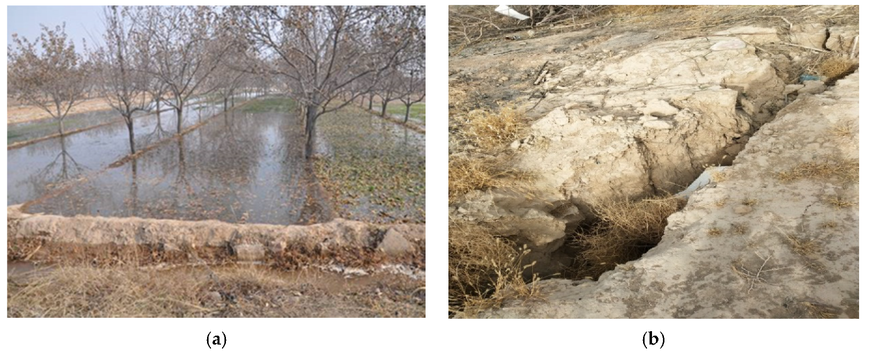
2.2.3. Hydrometeorology and Agricultural Irrigation

The study area is located in the northwest inland area, with a semi-arid climate in the middle temperate zone. The supply of precipitation to the groundwater in the area is very limited. In recent years, Heitai has become an important vegetable and fruit planting base. Economic crops that require more water have been mainly planted, and agricultural irrigation has been greatly increased (Figure 4a). However, irrigation infiltration increases the groundwater supply and destroys the groundwater balance field artificially. Along with the rise of the groundwater level, the thickness of the loess saturated zone increases year by year, which not only causes the overall collapse and landslides on the edge of the tableland but also causes cracks and sinkholes on the surface of the tableland (Figure 4b).

2.3. Basic Model Information

2.3.1. Generalization of the Boundary Conditions of the Calculation Model

The ground elevation, bottom elevation, and initial groundwater level elevation of the simulation area are shown in Figure 5a–c, respectively. There are 5 groundwater level holes (N4, N6, N8, N9, and N10) for monitoring, and their distribution is shown in Figure 5d. The main surface boundary conditions of the study area are rainfall, irrigation, and evaporation.

Table 1. Boundary conditions of the upper surface of the model ($\times {10}^{-4}$ m/day).

Month	7	8	9	10	11	12	1	2	3	4	5	6
Irrigation	5.81	5.45	2.63	0	3.00	0.16	0	0	0.55	3.37	4.35	7.50
Rainfall	1.79	2.26	1.27	0.55	0.07	0	0	0	0.26	0.53	1.19	1.37
Evaporation	6.97	6.19	4.27	3.23	2.17	1.26	1.29	1.39	4.06	6.67	7.13	7.10

shows the statistical data of each influencing factor in a hydrological year, and the irrigation water mainly comes from the Yellow River. The study area is the loess tableland, which is higher than its surroundings and is cut off by valleys. The loess aquifer can neither be supplied by the surface water nor by the lateral runoff of the groundwater outside the area. Some of the phreatic water in the loess layer is generally discharged in the form of a spring on the contact surface of the loess and silty clay, and the other part infiltrates to the sand gravel layer through the relatively impermeable silty clay layer. Therefore, the lateral direction of the model is generalized as the discharge boundary, which is achieved by the Drain module in MODFLOW. Because the permeability of the clay layer is very weak, the bottom of the model is generalized as a water barrier boundary.

2.3.2. Time Division of the Model

A total of 365 days of groundwater dynamic observation data in the simulation area, from 1 July 2016 to 31 June 2017, are selected for model parameter identification. The model is verified using another 365 days of groundwater dynamic observation data from 1 July 2017 to 30 June 2018. For the groundwater flow movement, each month is divided into three stress periods according to the actual situation, and the whole simulation period has 36 stress periods (

Table 2. Division of the stress periods in the groundwater flow model.

Month	7			8			9			10
Number of stress period	No.1	No.2	No.3	No.4	No.5	No.6	No.7	No.8	No.9	No.10	No.11	No.12
Length of stress period (day)	10	10	11	10	10	11	10	10	10	10	10	11
Month	11			12			1			2
Number of stress period	No.13	No.14	No.15	No.16	No.17	No.18	No.19	No.20	No.21	No.22	No.23	No.24
Length of stress period (day)	10	10	10	10	10	11	10	10	11	10	10	8
Month	3			4			5			6
Number of stress period	No.25	No.26	No.27	No.28	No.29	No.30	No.31	No.32	No.33	No.34	No.35	No.36
Length of stress period (day)	10	10	11	10	10	10	10	10	11	10	10	10

). Each stress period contains several time steps. In the simulation of the HYDRUS module, the initial time step is set to 0.01 day, and the minimum and maximum time steps are set to 1 $\times {10}^{-3}$ day and 0.1 day, respectively.

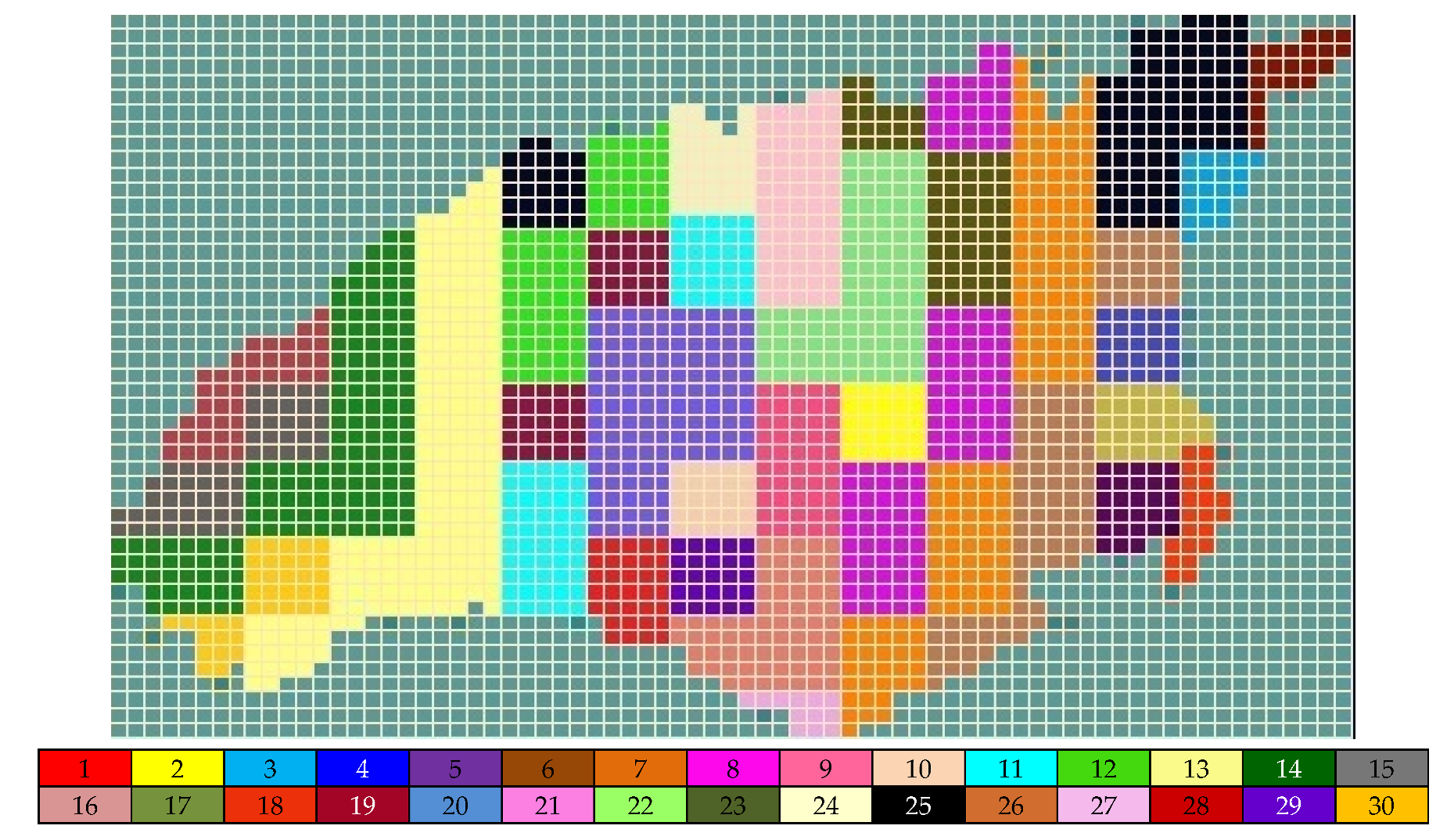
2.3.3. Spatial Division of the Model

In the horizontal direction, the model is divided into 47 rows and 73 columns. A total of 2275 of the 3431 units are active units, and the areas outside the boundary are treated as invalid units. Moreover, as shown in Figure 6, the simulation area is divided into 30 zones according to the surface elevation (Figure 5a) and the initial groundwater level (Figure 5c) of each unit. That is, the number of one-dimensional unsaturated profiles is 30. In the vertical direction, the HYDRUS profiles are divided into 84–125 finite elements with nodes at different depths.

3. Results and Discussion

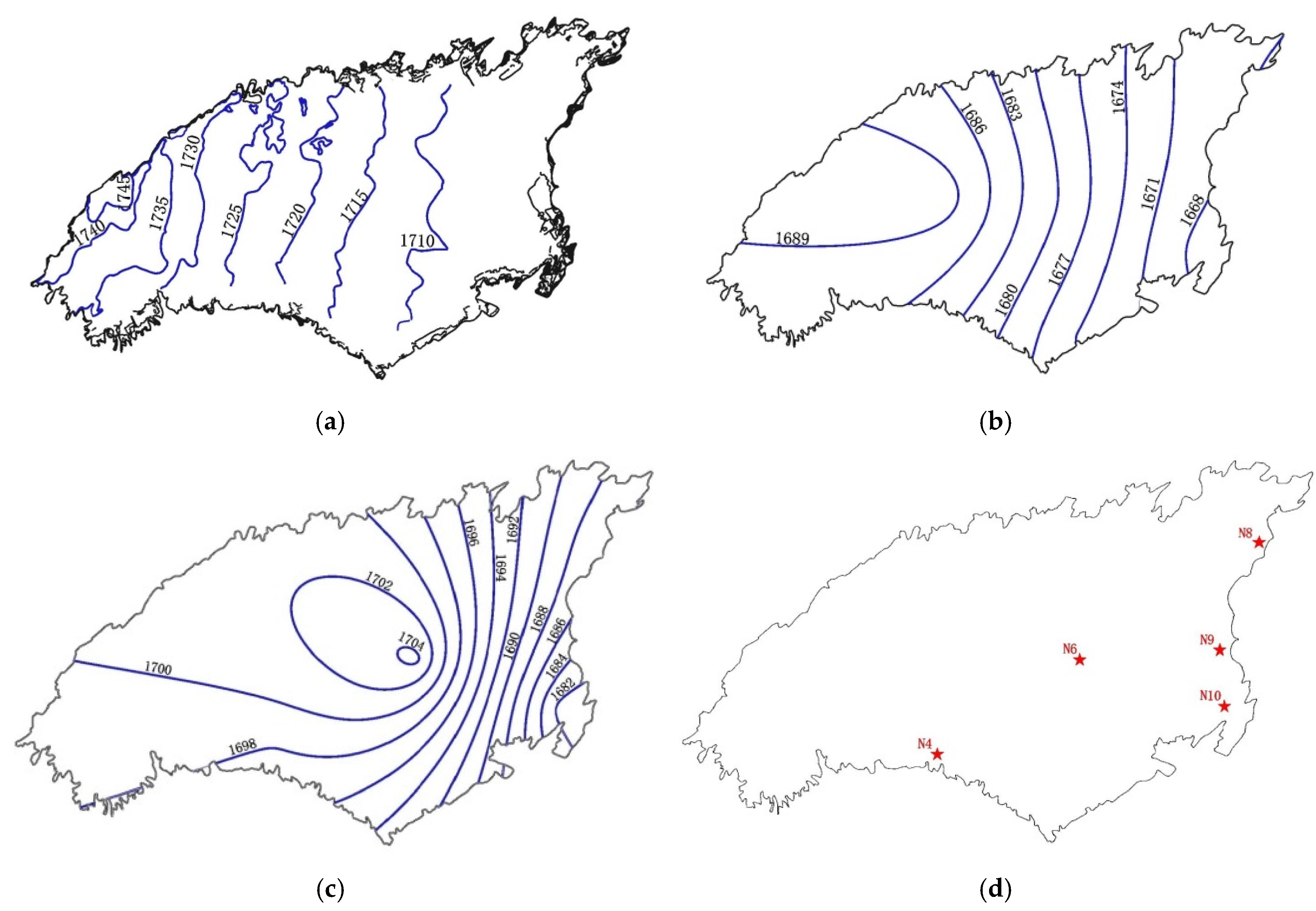
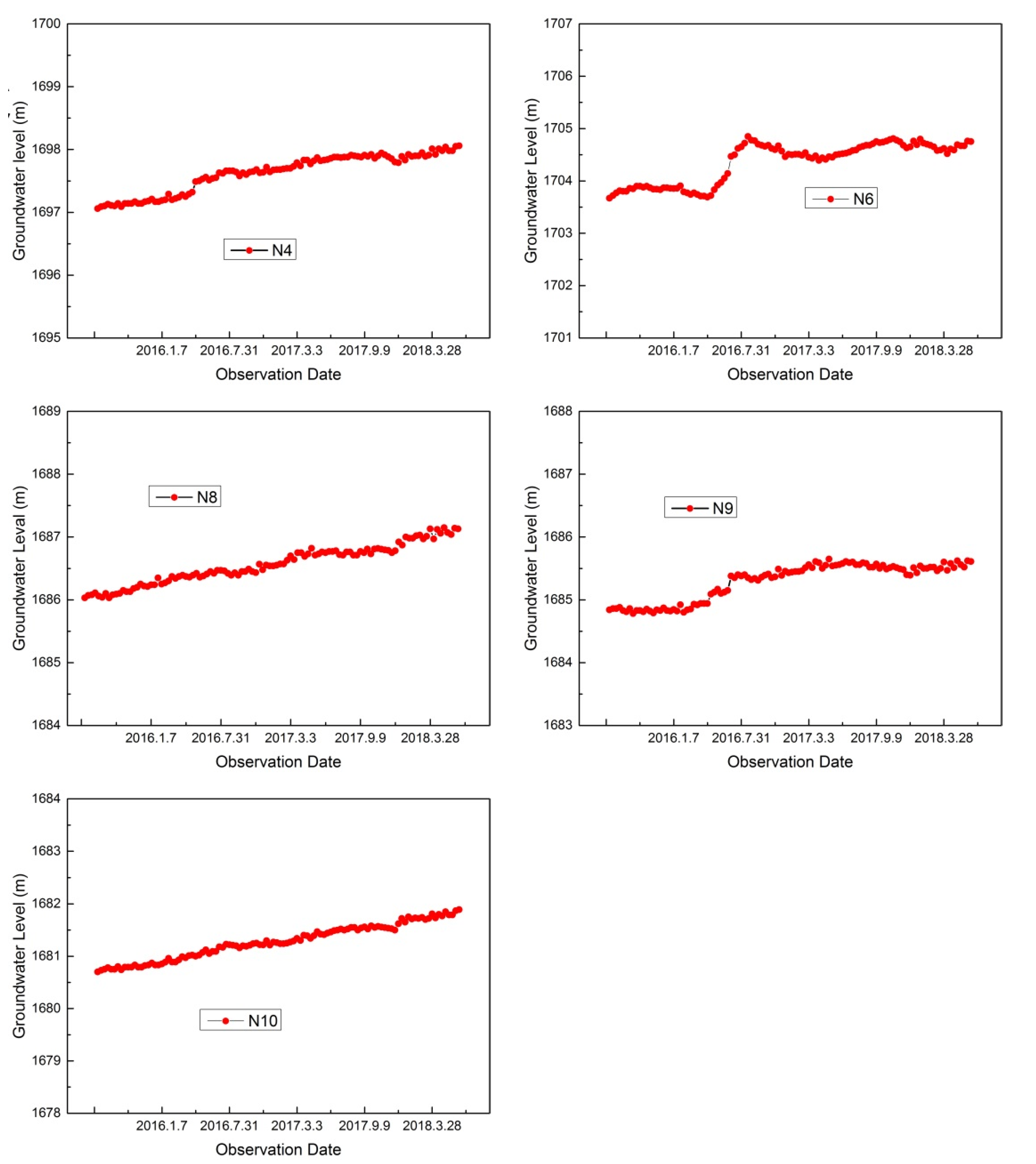
3.1. Dynamic Change of the Groundwater Level

Figure 7 shows the changes in the groundwater level at each groundwater level observation point from 1 July 2015 to 11 June 2018. The groundwater level in the Heitai area rises unevenly, and the rising rate in the middle of the tableland is faster than that at the edge of the tableland. Among them, the N6 point has the largest fluctuation amplitude of the groundwater level, which is mainly caused by the infiltration of irrigation water in the surrounding irrigation area. The groundwater level of the N9 also fluctuates obviously. In addition to the impact of vertical irrigation water, N9 is also recharged by the groundwater horizontally due to the terrain of the study area. At the N4 point, the groundwater level fluctuates slightly. The N8 and N10 points have no obvious fluctuation, which shows that they are mainly affected by the lateral recharge of groundwater and that the impact of irrigation recharge is weak.

3.2. Inversion Results of the Model Parameters

Due to the existence of vertical joints and fissures, loess is generalized as an anisotropic medium in a three-dimensional space, but it is generalized as an isotropic medium in the horizontal direction. The parameters required in the model and their optimized values obtained by the Bayesian-MCMC parameter inversion method are indicated in

Table 3. Model parameter values.

Types	${\mathsf{\theta }}_{\mathrm{r}}$	${\mathsf{\theta }}_{\mathbf{s}}$	$\mathsf{\alpha }$ (1/m)	n	Kx (m/day)	Kz (m/day)	Sy
Initial values	0.14	0.47	0.41	3.6	0.02	0.2	0.08
Prior ranges	[0.08, 0.15]	[0.45, 0.5]	[0.4, 0.5]	[3.1, 4.5]	[0.015, 0.025]	[0.15, 0.25]	[0.07, 0.09]
Optimized values	0.12	0.48	0.43	3.55	0.02	0.21	0.08

. The parameter values after inversion are basically consistent with the actual hydrogeological conditions in the area, and the model has high reliability.

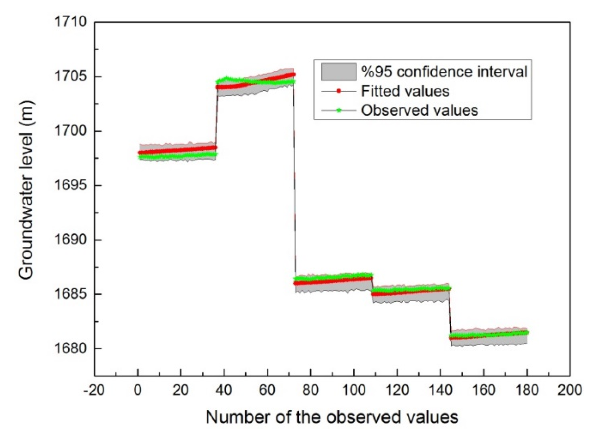
3.3. Simulation Results of the Groundwater Level and Model Verification

3.3.1. Groundwater Level Simulation Results

Model identification and validation is the key step to evaluate whether the model can truly reflect the hydrogeological conditions of the simulation area. The identification of the model allows repeated adjustment and modification of the hydrogeological parameters, boundary conditions, and source and sink terms of the model so that the model can more accurately reflect the actual hydrogeological conditions in the simulation area. Through the comparison of the actual measured groundwater level of the existing observation holes and the simulated ones, the variation trend and the difference between the two values are minimized. The fitting degree between the measured groundwater data of five observation holes in the study area and the simulated values is taken as the basis of model identification.

As we can see from Figure 8, the groundwater level during the simulation is simulated and compared with the measured values. We take 1 July 2016 to 30 June 2017, a total of 365 days, as the model validation period. The values at the end of every stress period are taken into consideration, and as a result, there are 18 groundwater level observations for each observation point and 90 groundwater level observations for five observation points in total. Figure 8 signifies that the groundwater level simulated by the HYDRUS-MODFLOW model fits well with the measured value. The evaluation index of the simulation effect RMSE = 0.34 m, so the simulation result of HYDRUS-MODFLOW at the regional scale is reliable, which indicates that the optimized model reflects the real dynamic change characteristics of the groundwater level. The observed values of the groundwater level are basically included in the 95% confidence interval, which indicates that the simulation uncertainty ranges are statistically adequate [37].

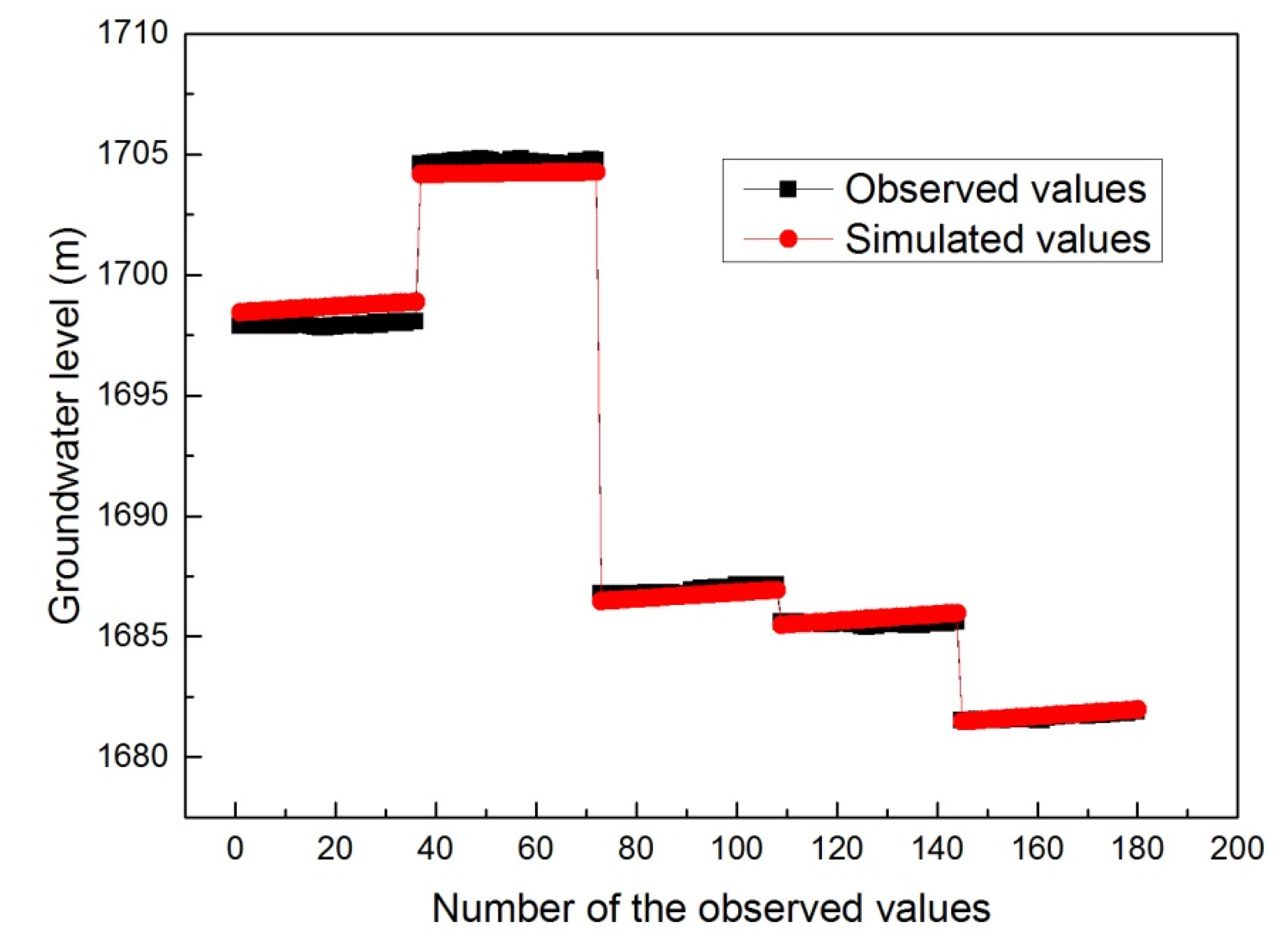
3.3.2. Model Validation

Before using the established model for simulation and prediction, we should first verify the model. We take 1 July 2017 to 30 June 2018 as the model validation period, a total of 365 days, to further verify the parameters of the optimized model. It can be seen from Figure 9 that the fitting effect between the calculated groundwater at each observation hole and the measured values during the model validation period is good. RMSE = 0.33 m indicates that the trend of the numerical simulation values of the Loess phreatic water level is close enough to the measured values. The model can accurately reflect the hydrogeological and dynamic characteristics of the simulation area from the perspective of the overall simulation situation and can be used for water level prediction. The simulation results show that the HYDRUS-MODFLOW model has a good simulation effect on the water exchange process between saturated and unsaturated zones at the regional scale, which is consistent with Reference [24].

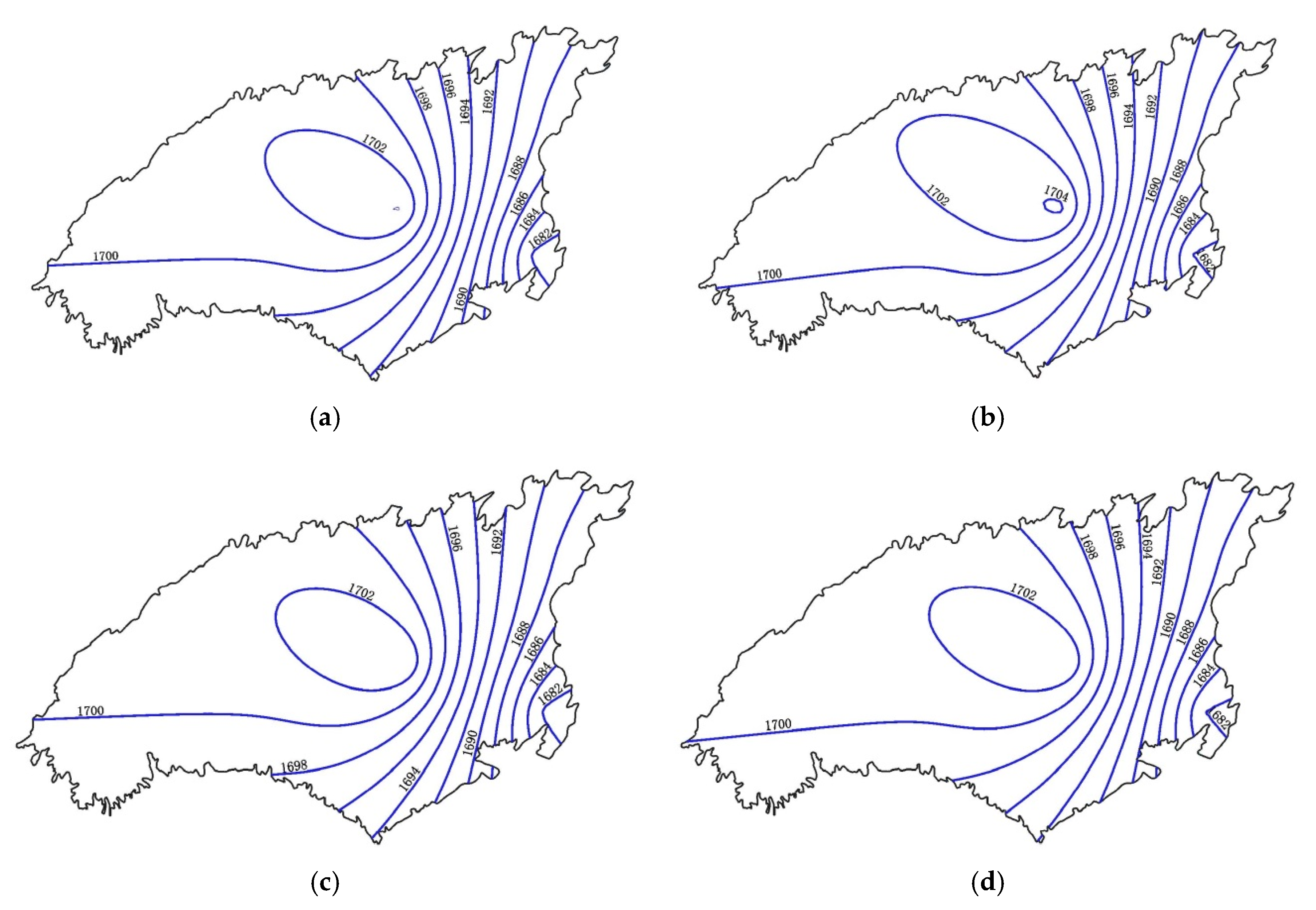
3.4. Prediction of the Groundwater Level Change Trend

Using the above optimized model, we can predict the change of the groundwater level under different irrigation conditions. In this paper, the change of the groundwater level in the study area over 3 years is predicted under the condition that the irrigation amount is 1 times and 0.8 times the initial irrigation amount. Figure 10 shows the distribution of the groundwater flow field in the first year and the third year under the conditions of different irrigation volumes.

It can be seen from Figure 10 that under the condition of the original irrigation amount and 0.8 times the original irrigation amount, the contour of the groundwater level obviously shifts right, that is, the groundwater level rises with time. Among these, the contour of the 1702 m groundwater level on the left side expands with the increase of the simulation time. However, under the condition of the original irrigation, the movement of the groundwater level contour is more obvious. The results fully show that a reasonable reduction of irrigation can effectively slow down the continuous rise of the groundwater level.

Under the influence of long-term irrigation, the groundwater level of Heitai is rising year by year, which leads to many landslides along the border of the tableland [4]. Treatments such as slope cutting and load reduction have been carried out in this area and potential deformation bodies have been temporarily removed. However, because the hydrogeological conditions have not fundamentally changed, the slope body is likely to undergo a potential deformation at any time. Through the discussion in the previous section, it is concluded that a reasonable reduction of irrigation can effectively slow down the continuous rise of the groundwater level. There are many ways to reduce the amount of irrigation: first, we should change the method of irrigation, reducing flood irrigation to prevent water waste; second, we should improve the type of crops planted, planting more types of crops with strong drought resistance and less water demand. Simultaneously while reducing agricultural irrigation, other measures should also be taken to help reduce the groundwater level. Direct groundwater drainage schemes are the most effective and direct measures for landslide disaster control.

4. Conclusions

The main conclusions of this study are:

• On the basis of the coupling principle and operation mechanism of the HYDRUS-MODFLOW coupling model, the model is applied to simulate the groundwater level of Heitai in Gansu Province. The simulation results show that the HYDRUS-MODFLOW model has a good simulation effect on the water exchange process between saturated and unsaturated zones at the regional scale.
• To further improve the practicability and simulation accuracy of the HYDRUS-MODFLOW model, it is combined with the Bayesian-MCMC parameter inversion method. The parameters in the model are inverted and verified using the measured groundwater level data in the field water level holes. The results show that the simulation values of the coupling model fit well with the measured values, which indicates that the model can better simulate the transformation relationship among surface water, soil water, and groundwater at the regional scale in Heitai.
• The development trend of the groundwater level of the Heitai groundwater system in Gansu Province in the next 3 years under different irrigation intensities is predicted using the optimized model. The prediction results show that the groundwater level is seriously affected by the irrigation intensity. The groundwater level increases with the increase of the irrigation intensity and decreases with the decrease of the irrigation intensity. A reasonable reduction of the irrigation intensity can slow the rising speed of the groundwater level.
• Measures to reduce the groundwater level in Heitai are recommended, such as reasonable reduction of the irrigation amount by changing the irrigation mode; adjustment of the crop structure and planting area to reduce uneven irrigation as much as possible; and direct discharge of groundwater by adopting the drainage test scheme.

References

1. Gu, T.; Wang, J.; Wang, C.; Bi, Y.; Guo, Q.; Liu, Y. Experimental study of the shear strength of soil from the Heifangtai Platform of the Loess Plateau of China. J. Soils Sediments 2019, 19, 3463–3475. [Google Scholar] [CrossRef]
2. Meng, Q.; Xu, Q.; Wang, B.; Li, W.; Peng, Y.; Peng, D.; Qi, X.; Zhou, D. Monitoring the regional deformation of loess landslides on the Heifangtai terrace using the Sentinel-1 time series interferometry technique. Nat. Hazards 2019, 98, 485–505. [Google Scholar] [CrossRef]
3. Liu, X.; Zhao, C.; Zhang, Q.; Yang, C.; Zhu, W. Heifangtai loess landslide type and failure mode analysis with ascending and descending Spot-mode TerraSAR-X datasets. Landslides 2020, 17, 205–215. [Google Scholar] [CrossRef] [Green Version]
4. Xu, L.; Dai, F.C.; Gong, Q.M.; Tham, L.G.; Min, H. Irrigation-induced loess flow failure in Heifangtai Platform, North-West China. Environ. Earth Sci. 2012, 66, 1707–1713. [Google Scholar] [CrossRef]
5. Leng, Y.; Peng, J.; Wang, Q.; Meng, Z.; Huang, W. A fluidized landslide occurred in the Loess Plateau: A study on loess landslide in South Jingyang tableland. Eng. Geol. 2018, 236, 129–136. [Google Scholar] [CrossRef]
6. Cui, S.; Pei, X.; Wu, H.; Huang, R. Centrifuge model test of an irrigation-induced loess landslide in the Heifangtai loess platform, Northwest China. J. Mt. Sci. 2018, 15, 130–143. [Google Scholar] [CrossRef]
7. Arnold, J.G.; Allen, P.M.; Bernhardt, G. A comprehensive surface-groundwater flow model. J. Hydrol. 1993, 142, 47–69. [Google Scholar] [CrossRef]
8. Sophocleous, M. Interactions between groundwater and surface water: The state of the science. Hydrogeol. J. 2002, 10, 52–67. [Google Scholar] [CrossRef]
9. Li, W.; He, J. Analysis of Relation and Variation Characteristics Between Soil Water and Groundwater in Planting Conditions. Earth Sci. 2015, 4, 235–240. [Google Scholar] [CrossRef]
10. Chen, X.; Hu, Q. Groundwater influences on soil moisture and surface evaporation. J. Hydrol. 2004, 297, 285–300. [Google Scholar] [CrossRef] [Green Version]
11. Xie, W.; Yang, J. Assessment of Soil Water Content in Field with Antecedent Precipitation Index and Groundwater Depth in the Yangtze River Estuary. J. Integr. Agric. 2013, 12, 711–722. [Google Scholar] [CrossRef]
12. Ramos, T.B.; Simionesei, L.; Jauch, E.; Neves, R. Modelling soil water and maize growth dynamics influenced by shallow groundwater conditions in the Sorraia Valley region, Portugal. Agric. Water Manag. 2017, 185, 27–42. [Google Scholar] [CrossRef]
13. Chen, Z.; Govindaraju, R.S.; Kavvas, M.L. Spatial averaging of unsaturated flow equations under infiltration conditions over areally heterogeneous fields: 1. Development of models. Water Resour. Res. 1994, 30, 523–533. [Google Scholar] [CrossRef]
14. Chen, Z.; Govindaraju, R.S.; Kavvas, M.L. Spatial averaging of unsaturated flow equations under infiltration conditions over areally heterogeneous fields: 2. Numerical simulations. Water Resour. Res. 1994, 30, 535–548. [Google Scholar] [CrossRef]
15. Sherlock, M.D.; McDonnell, J.J.; Curry, D.S.; Zumbuhl, A.T. Physical controls on septic leachate movement in the vadose zone at the hillslope scale, Putnam County, New York, USA. Hydrol. Process. 2002, 16, 2559–2575. [Google Scholar] [CrossRef]
16. Sophocleous, M.A.; Koelliker, J.K.; Govindaraju, R.S.; Birdie, T.; Ramireddygari, S.R.; Perkins, S.P. Integrated numerical modeling for basin-wide water management: The case of the Rattlesnake Creek basin in south-central Kansas. J. Hydrol. 1999, 214, 179–196. [Google Scholar] [CrossRef]
17. Semiromi, M.T.; Koch, M. Analysis of spatio-temporal variability of surface–groundwater interactions in the Gharehsoo river basin, Iran, using a coupled SWAT-MODFLOW model. Environ. Earth Sci. 2019, 78, 201. [Google Scholar] [CrossRef]
18. Kim, N.W.; Chung, I.M.; Won, Y.S.; Arnold, J.G. Development and application of the integrated SWAT-MODFLOW model. J. Hydrol. 2008, 356, 1–16. [Google Scholar] [CrossRef]
19. Facchi, A.; Ortuani, B.; Maggi, D.; Gandolfi, C. Coupled SVAT–groundwater model for water resources simulation in irrigated alluvial plains. Environ. Modell. Softw. 2004, 19, 1053–1063. [Google Scholar] [CrossRef]
20. Kuznetsov, M.; Yakirevich, A.; Pachepsky, Y.A.; Weisbrod, N. Quasi 3D modeling of water flow in vadose zone and groundwater. J. Hydrol. 2012, 450, 140–149. [Google Scholar] [CrossRef]
21. Bushira, K.M.; Hernandez, J.R.; Sheng, Z. Surface and groundwater flow modeling for calibrating steady state using MODFLOW in Colorado River Delta, Baja California, Mexico. Model. Earth Syst. Environ. 2017, 3, 815–824. [Google Scholar] [CrossRef]
22. Lekula, M.; Lubczynski, M.W. Use of remote sensing and long-term in-situ time-series data in an integrated hydrological model of the Central Kalahari Basin, Southern Africa. Hydrogeol. J. 2019, 27, 1541–1562. [Google Scholar] [CrossRef] [Green Version]
23. Cheng, Q.; Chen, X.; Chen, X.; Zhang, Z.; Ling, M. Water infiltration underneath single-ring permeameters and hydraulic conductivity determination. J. Hydrol. 2011, 398, 135–143. [Google Scholar] [CrossRef]
24. Twarakavi, N.K.C.; Šimůnek, J.; Seo, S. Evaluating Interactions between Groundwater and Vadose Zone Using the HYDRUS-Based Flow Package for MODFLOW. Vadose Zone J. 2008, 7, 757–768. [Google Scholar] [CrossRef] [Green Version]
25. Khu, S.T.; Werner, M.G.F. Reduction of Monte-Carlo Simulation Runs for Uncertainty Estimation in Hydrological Modelling. Hydrol. Earth Syst. Sci. 2003, 7, 680–692. [Google Scholar] [CrossRef] [Green Version]
26. Arridge, S.R.; Kaipio, J.P.; Kolehmainen, V.; Schweiger, M.; Somersalo, E.; Tarvainen, T.; Vauhkonen, M. Approximation errors and model reduction with an application in optical diffusion tomography. Inverse Probl. 2006, 22, 175–195. [Google Scholar] [CrossRef] [Green Version]
27. Ekblad, J.; Isacsson, U. Time-domain Reflectometry Measurements and Soil-water Characteristic Curves of Coarse Granular Materials Used in Road Pavements. Can. Geotech. J. 2007, 44, 858–872. [Google Scholar] [CrossRef]
28. Vrugt, J.A.; Stauffer, P.H.; Wöhling, T.; Robinson, B.A.; Vesselinov, V.V. Inverse Modeling of Subsurface Flow and Transport Properties: A Review with New Developments. Vadose Zone J. 2008, 7, 843–864. [Google Scholar] [CrossRef]
29. Godoy, V.A.; Zuquette, L.V.; Gómez-Hernández, J.J. Scale effect on hydraulic conductivity and solute transport: Small and large-scale laboratory experiments and field experiments. Eng. Geol. 2018, 243, 196–205. [Google Scholar] [CrossRef]
30. Tarantino, A.; Ridley, A.M.; Toll, D.G. Field Measurement of Suction, Water Content, and Water Permeability. Geotech. Geol. Eng. 2008, 26, 751–782. [Google Scholar] [CrossRef]
31. Zeng, L.; Shi, L.; Zhang, D.; Wu, L. A sparse grid based Bayesian method for contaminant source identification. Adv. Water Resour. 2012, 37, 1–9. [Google Scholar] [CrossRef]
32. Man, J.; Liao, Q.; Zeng, L.; Wu, L. ANOVA-based transformed probabilistic collocation method for Bayesian data-worth analysis. Adv. Water Resour. 2017, 110, 203–214. [Google Scholar] [CrossRef]
33. Levenberg, K. A Method for the Solution of Certain Non-linear Problems in Least Squares. Q. Appl. Math. 1944, 2, 164–168. [Google Scholar] [CrossRef] [Green Version]
34. Maier, H.R.; Kapelan, Z.; Kasprzyk, J.; Kollat, J.; Matott, L.S.; Cunha, M.C.; Dandy, G.C.; Gibbs, M.S.; Keedwell, E.; Marchi, A.; et al. Evolutionary algorithms and other metaheuristics in water resources: Current status, research challenges and future directions. Environ. Modell. Softw. 2014, 62, 271–299. [Google Scholar] [CrossRef] [Green Version]
35. Over, M.W.; Wollschläger, U.; Osorio-Murillo, C.A.; Rubin, Y. Bayesian inversion of Mualem-van Genuchten parameters in a multilayer soil profile: A data-driven, assumption-free likelihood function. Water Resour. Res. 2015, 51, 861–884. [Google Scholar] [CrossRef]
36. Harbaugh, A.W.; Banta, E.R.; Hill, M.C.; McDonald, M.G. MODFLOW-2000, The US Geological Survey Modular Ground-Water Model—User Guide to Modularization Concepts and the Ground-Water Flow Process; Open-File Report 00-92; USGS: Reston, VA, USA, 2000.
37. Vrugt, J.A. Markov chain Monte Carlo simulation using the DREAM software package: Theory, concepts, and MATLAB implementation. Environ. Modell. Softw. 2016, 75, 273–316. [Google Scholar] [CrossRef] [Green Version]
Figure 1. Schematic diagram of the HYDRUS-MODFLOW coupling principle.
Water 12 02546 g001
Figure 2. Geographical location of the study area.
Water 12 02546 g002
Figure 3. Front edge of Heitai.
Water 12 02546 g003
Figure 4. Heitai irrigation area: (a) flood irrigation; (b) ground crack.
Water 12 02546 g004
Figure 5. Study area: (a) Contour of the top elevation; (b) contour of the bottom elevation of the loess layer; (c) contour of the initial groundwater level; (d) distribution of the observation holes for the groundwater level.
Water 12 02546 g005
Figure 6. Spatial grid division and the HYDRUS module zones.
Water 12 02546 g006
Figure 7. Variation of the groundwater level elevation with time at each observation hole.
Water 12 02546 g007
Figure 8. Fitting result of the groundwater level.
Water 12 02546 g008
Figure 9. Observations and fitting values of the groundwater level in the model validation period.
Water 12 02546 g009
Figure 10. Changes of the groundwater level under different irrigation conditions (m): (a) the first year under the original irrigation amount; (b) the third year under the original irrigation amount; (c) the first year under 0.8 times the original irrigation amount; (d) the third year under 0.8 times the original irrigation amount.
Water 12 02546 g010